Sage Journals: Discover world-class research

Abstract

This article investigates the impacts of changes in the U.S.-implied volatility on the changes in implied volatilities of the Euro and Thai stock markets. For that purpose, volatilities implicit in stock index option prices from the United States, Euro, and Thai stock markets are analyzed using the Standard Granger Causality Test, impulse response analysis, and variance decompositions. The results found in this study suggest that the U.S. stock market is the leading source of volatility transmissions since the changes in implied volatility in the U.S. stock market are transmitted to the Euro and Thai stock markets. Implied volatility indexes are used because they contain information about future realized volatility beyond that contained past volatility. Therefore, implied volatility indexes can be used as an underlying asset in a derivative market. The risk factors that can gauge the expectations of institutional investors are important to the key players in international stock markets. Given the dominance of institutional traders in the international derivative markets, the implied volatilities should reflect international traders’ sentiment. The findings in the present article give recent knowledge for portfolio managers because they need to know the degree of dependency across stock markets so that they can diversify more efficiently.

Keywords

stock index option prices implied volatility causality impulse response functions variance decompositions

Introduction

Empirically, return and volatility transmissions across stock markets based on market returns and volatilities are investigated to find the degree of stock market integration using various econometric techniques. The econometric techniques include Cointegration Test, Causality Test, generalized autoregressive conditional heteroscedastic (GARCH) model estimation, correlation, and regression analyses. For example, Liu and Pan (1997) use a GARCH model to examine the mean return and volatility spillover effects from the U.S. and Japanese stock markets to four Asian stock markets (those of Hong Kong, Singapore, Taiwan, and Thailand). Their main finding indicates that the U.S. stock market is more influential in transmitting return and volatility to the four Asian markets. Raj and Dhal (2008) find high correlations of stock price indices that strengthen the integration of India’s stock market with global and regional markets. Furthermore, the absolute size of coefficients in the long-run relationship suggests that the Indian stock market is dependent on global markets, that is, the U.S. and U.K. stock markets. Besides, Chiang, Jeon, and Li (2007) use dynamic correlation analysis and find evidence for the contagion effects between Asian markets. However, there is an argument that implied volatility as a measure of volatility or uncertainty in a stock market can be more useful. According to Fleming, Ostdiek, and Whaley (1995) and Whaley (2000), implied volatility is affected by both positive and negative return shocks. This implied volatility index falls for positive return shocks and rises for negative return shocks. Bollerslev and Zhou (2006) find that the asymmetric response of current volatility to lagged negative and positive returns is stronger for implied volatility than realized volatility. Blair, Poon, and Taylor (2001) also find that applying implied volatility is useful when predicting future volatilities. The evidence of a negative relationship between stock index return and its corresponding implied volatility can be found in Giot (2005) and Badshah (2013).

Nikkinen and Sahlström (2004) use implied volatility indices test for market integration. They find a high degree of integration among the U.S., U.K., and German stock markets. The U.S. stock market transmits volatility to the other markets whereas German market transmits volatility to the other European stock markets. Recent empirical studies using different methods show that financial shocks play an important role in spillover effects among stock markets. Peng and Ng (2012) find evidence of financial contagion in five popular indices of advance stock markets. The degree of dependency is influenced by financial shocks. Siriopoulos and Fassas (2013) use dynamic conditional correlation to examine the spillover effects across international financial markets using implied volatility indices. They find that capital market integration increases in the periods of financial turbulence. Kenourgios (2014) uses the data set from a sample of international implied volatility indices on daily changes basis and finds evidence indicating the existence of contagion in cross-market volatilities. The most contagious phase is the early phase of global financial crisis.

The Thai stock market, namely, the Stock Exchange of Thailand (SET), is an emerging stock market in Southeast Asia. Established in 1974, this stock market has been gradually developed. The implementation of financial liberalization in 1992 has induced increasing capital inflows to the market in terms of portfolio investment. Like other emerging stock markets, the SET can be affected by various economic forces, which cause a swing in stock prices of listed companies in most economic sectors. The main sub-index in the SET is the SET50 index, has been constructed so as to accommodate the availability of index options. The SET50 index options can be used to hedge against risk in the Thai stock market by both local and foreign investors.

The main purpose of the present study is to investigate implied volatility transmissions among international stock market. The rationale for using implied volatility index is that this index indicates the consensual view about the expected future realized stock index volatility as suggested by Whaley (2000). The present study contributes to the existing literature by providing evidence of implied volatility transmissions between an emerging stock market (the SET) and two international stock markets (those of the U.S. and Euro markets). The methods used in the analysis are similar to those of Nikkinen and Sahlström (2004), Äijö (2008), and Siriopoulos and Fassas (2012). Unlike cointegration techniques, the vector autoregressive (VAR) model along with the Standard Causality Test allow for directly examining implied volatility spillovers among international stock markets. The Causality Test can also trace the impacts of lagged variables on current variables. In addition, the VAR model can be used to analyze impulse response functions and variance decompositions, which are useful in capturing how a unit shock of one variable can affect other variables and how other variables respond to a unit shock of that variable. The period of investigation is during November 2010 to December 2013. The justification for using the specified period is that the available data set is limited by the emergence of SET50 index option prices in November 2010. Furthermore, the study period also includes the period of the U.S. subprime crisis that might affect other international stock markets. The main findings of the present study are that (a) the impact of the subprime crisis in the United States does not affect the results of the analyses, (b) there is a unidirectional causality running from the U.S.-implied volatility changes to those of the Euro and Thai stock markets, and (c) the impulse response analysis and variance decompositions seem to support the results from causality analysis. The next section presents the methodology used in this study. “Empirical Results” section presents the empirical results, and the last section gives concluding remarks.

Method

Data

This study uses daily data during November 2010 to December 2013. The prices of SET50 index options are used as an emerging market index, that is, major sub-index of the SET. The implied volatility indexes of the large two international stock markets are the Euro STOXX50 index and the U.S. S&P500 implied volatility index. The number of observations is 634. The number of observations is limited by the availability of the price of the SET50 index options that will be used to estimate the implied volatility index. The SET50 index is calculated from stock prices of the top 50 listed companies with large market capitalization in the SET. The data set is obtained from SETSMART (SET Market Analysis and Reporting Tools) and Thomson Financial DataStream.

Practically, the implied volatility index indicates the consensus view about the expected future realized stock index volatility (see, for example, Whaley, 2000). Implied volatility indexes are typically available in advanced stock markets, but the implied volatility index is not available in Thailand. Therefore, this index is calculated using the Black and Sholes (1973) option pricing formula, which is the most widely used because of its consistency with the assumption that investors in an option market behave as if they use this formula to evaluate the option prices (see Christensen & Prabhala, 1998, among others). The valuation model of option is specified as

C (S, t) = S N (d_{1}) - K e^{- r (t - T)} N (d_{2}),

where C is the option price, S is the current stock price, K is the option striking price or exercise price, r is the risk-free rate, and T is the expiration date of the option. The cumulative normal density functions (Ns) of two variables, d₁ and d₂, are normally distributed with a mean of zero and a standard deviation of one. These variables are specified as

d_{1} = \frac{[\ln (\frac{S}{K}) + (r + \frac{1}{2} σ_{S}^{2}) (T - t)]}{σ_{S} \sqrt{(T - t)}}

and

d_{2} = d_{1} - σ_{S} \sqrt{(T - t)},

where σ_S is the standard deviation of stock price. The expression $S N (d_{1}) e^{- r (T - t)}$ is the expected value that is equal to S_T if S_T > K and zero otherwise. The function N(d₂) is the probability that the option will be exercised so that KN(d₂) is the striking price multiplied by the probability that the striking price will be paid.

One of various parameters in the Black and Sholes pricing formula that cannot be directly observed is the volatility of the underlying stock price. However, it is possible to gauge such a volatility value that causes the option value to be consistent with the market price of an option. In calculating the implied volatility in a stock market, one can plug in the values of all parameters in the option pricing formula, including the option price from an option market. Then the iterative procedure can be used to calculate the implied volatility such that the option price obtained from the formula is equal to the actual option price observed in the option market (Watsham & Parramore, 1997). Because the established volatility is the implied volatility for each individual option at each exercise price, the implied volatility index should be computed as an average of all individual implied volatilities from the at-the-money options or near-the-money options. Such calculation is consistent with the fact that the price of at-the-money option is far more sensitive to volatility than the price of deep-out-of-the-money option. According to Hull (1997), this calculated volatility is more informative to the true implied volatility.

Table 1 presents the descriptive statistics of implied volatilities in the four stock markets. Panel A of Table 1 presents the sample properties of implied volatility series in their level. The descriptive statistics show that implied volatility series are generally similar because all series have positive means with high kurtosis. However, first differences of all series exhibit small values of negative means, but with higher standard deviation as shown in Panel B of Table 1. It should be noted that the means of implied volatility of the three markets are low, but exhibit excess kurtosis.

Table 1.

Descriptive Statistics of Implied Volatilities (November 2010-December 2013).

	v^US	v^Euro	v^TH
Panel A: Level
M	0.187	0.243	0.218
Median	0.170	0.223	0.210
Maximum	0.480	0.504	0.486
Minimum	0.113	0.141	0.082
SD	0.063	0.075	0.068
Skewness	1.862	1.362	0.882
Kurtosis	6.333	4.441	3.967
Panel B: Difference
M	−8.8E−05	−8.8E−05	−2.7E−05
Median	−0.0007	−0.0008	−0.0004
Maximum	0.1600	0.1213	0.2280
Minimum	−0.0889	−0.1066	−0.1686
SD	0.0179	0.0191	0.0295
Skewness	1.6249	0.3512	0.9373
Kurtosis	17.8339	9.0204	19.5125

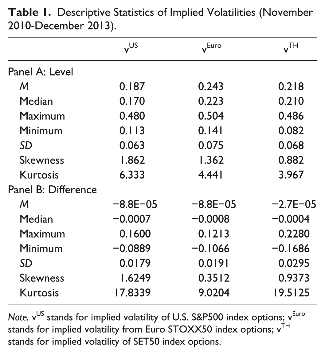
Note. v^US stands for implied volatility of U.S. S&P500 index options; v^Euro stands for implied volatility from Euro STOXX50 index options; v^TH stands for implied volatility of SET50 index options.

The implied volatilities of the three stock markets during the sample period are illustrated in Figure 1.

Figure 1.

Implied volatilities of the U.S., Euro, and Thai stock markets.

Figure 1 shows the plots of uneven implied volatilities of the three markets. However, the patterns of implied volatilities of the U.S. and Euro stock markets are similar. The implied volatility of the Thai stock market seems to be different from the other two markets.

To examine the stationarity property of implied volatilities, the Augmented Dickey and Fuller (ADF) and Phillips and Perron (PP) tests with a constant are applied. Table 2 presents the results of Unit Root Test without a linear trend.

Table 2.

Results of Unit Root Tests.

	ADF statistic	PP statistic
Panel A: Level of implied volatility
v^US	−1.962 [12]	−3.274 [2]
	(.304)	(.017)**
v^Euro	−2.170 [4]	−2.546 [4]
	(.218)	(.105)
v^TH	−2.840 [3]	−4.813 [10]
	(.000)***	(.000)***
Panel B: Difference of implied volatility
Δv^US	−8.409 [11]	−29.897 [14]
	(.304)***	(.000)***
Δv^Euro	−16.472 [3]	−26.881 [25]
	(.000)***	(.000)***
Δv^TH	−16.752 [3]	−43.294 [15]
	(.000)***	(.000)***

Note. The number in brackets is the optimal lag length determined by AIC for the ADF test and the optimal bandwidth determined by the Bartlett kernel for the PP Test. The number in parenthesis is the p value. ADF = Augmented Dickey and Fuller; PP = Phillips and Perron; v^US stands for implied volatility of U.S. S&P500 index options; v^Euro stands for implied volatility from Euro STOXX50 index options; v^TH stands for implied volatility of SET50 index options; AIC = Akaike information criterion.

***

and ** denote 1% and 5% significance level, respectively.

The results of Unit Root Tests in Panel A of Table 2 give mixed results for the four implied volatility series. However, the results in Panel B of Table 2 indicate that changes in all implied volatilities are stationary. Therefore, differences of implied volatility series are used in the analysis.

Analytical Framework

This study uses the VAR model proposed by Sim (1980), which is suitable to estimate the relationships among variables. In addition, Granger (1969) Causality Test is used to determine the direction of causality between stationary variables in the model. Following the works of Nikkinen and Sahlström (2004), Äijö (2008), and Siriopoulos and Fassas (2012), the VAR(p) model can be expressed as

Δ y_{t} = μ + \sum_{i = 1}^{p} A_{i} Δ y_{t - i} + e_{t},

where Δy is a 3 × 1 vector of changes in implied volatilities (Δv), μ is a 3 × 1 vector of intercepts, {A_i, I = 1,2,…} is a 3 × 3 matrix of autoregressive coefficients, and e is a 3 × 1 vector of random errors with zero means and positive definitive co-variances. The optimal lag p can be determined by Akaike information criterion (AIC), Schwarz information criterion (SIC), or final prediction error (FPE).

In examining the spillovers of implied volatilities from one stock market to another stock market, one can use this VAR system to analyze the time structure of transmissions under the assumption that there exist causal relationships between implied volatilities. Equation 4 is used to examine the dynamic impact of random innovations on a system of variables. The specified VAR model treats each endogenous variable in the system as a function of lagged endogenous variables in dynamic simultaneous equations.

Empirical Results

The Standard Granger Causality Test and VAR(p) estimation are performed on first differences of implied volatilities. Even though the implied volatility series for Thailand is found to be stationary at level, other series are not stationary at level. Therefore, using first differences of all series are suitable in performing Causality Test because the test requires that all series be strictly stationary. To perform Causality Test, the appropriate lag length needs to be determined. Table 3 presents the lag order selection for VAR(p) model. While AIC and FPE give the optimal lag of four, SIC gives the optimal lag of two. Because the Breusch–Godfrey Lagrange Multiplier (LM) test shows that the VAR system with the lag of four indicates no serial correlation, the lag of four is applied in the VAR analysis and Granger Causality Test.

Table 3.

Criteria for Lag Order Selection of VAR(p) Model.

Lag	AIC	SIC	FPE
0	−15.106	−15.085	−5.52E−11
1	−15.427	−15.342	−4.01E−11
2	−15.516	−15.367^a	−3.67E−11
3	−15.573	−15.360	−3.46E−11
4	−15.577^a	−15.301	−3.45E−11^a
5	−15.564	−15.223	−3.49E-11
6	−15.547	−15.142	−3.55E−11
7	−15.533	−15.064	−3.60E−11
8	−15.534	−15.001	−3.60E−11

Note. VAR = vector autoregressive; AIC = Akaike information criterion; SIC = Schwarz information criterion; FPE = final prediction error.

Indicates the optimal lag length for each criterion.

The results of Granger Causality Test are reported in Table 4. The test shows directions of causality between each pair of changes in implied volatilities.

Table 4.

Results of Granger Causality Test.

Null hypothesis	F statistic	p value
v^US does not Granger cause v^Euro	12.256	.000***
v^Euro does not Granger cause v^US	0.531	.713
v^US does not Granger cause v^TH	2.273	.060*
v^TH does not Granger cause v^US	1.314	.263
v^Euro does not Granger cause v^TH	1.023	.395
v^TH does not Granger cause v^Euro	1.186	.316

Note. The test is performed on changes in implied volatility. v^US stands for implied volatility of U.S. S&P500 index options; v^Euro stands for implied volatility from Euro STOXX50 index options; v^TH stands for implied volatility of SET50 index options.

***

, **, and * indicate significance at the 1%, 5%, and 10%, respectively.

The results in Table 4 show that the implied volatility of the U.S. stock market causes implied volatilities of Euro and Thai stock markets. However, implied volatilities of Thai and Euro stock markets do not cause implied volatilities of the U.S. stock market. Therefore, it can be concluded that implied volatility transmits from the U.S. stock market to the Euro and Thai stock markets.

To analyze the predictability and implied volatility transmissions of the three stock markets in more detail, the impulse response functions and variance decompositions are obtained from the VAR(4) model. The summary statistics of the results from the VAR(4) model estimate are presented in Table 5.

Table 5.

Summary Statistics of the Results From the VAR(4) Model Estimate.

	Δv^US	Δv^Euro	Δv^TH
Δv^US(−1)	−0.186***	0.382***	0.164*
	(0.058)	(0.060)	(0.091)
Δv^US(−2)	−0.189***	0.119*	−0.108
	(0.064)	(0.066)	(0.100)
Δv^US(−3)	−0.275***	−0.052	−0.073
	(0.064)	(0.067)	(0.067)
Δv^US(−4)	−0.169**	−0.071	0.001
	(0.060)	(0.062)	(0.093)
Δv^Euro(−1)	0.049	−0.263***	0.004
	(0.056)	(0.059)	(0.088)
Δv^Euro(−2)	0.054	−0.237***	0.067
	(0.058)	(0.060)	(0.091)
Δv^Euro(−3)	0.065	−0.008	0.118
	(0.058)	(0.061)	(0.092)
Δv^Euro(−4)	0.003	−0.065	−0.014
	(0.052)	(0.054)	(0.081)
Δv^TH(−1)	0.031	0.025	−0.444***
	(0.026)	(0.027)	(0.041)
Δv^TH(−2)	0.038	0.031	−0.287***
	(0.029)	(0.030)	(0.045)
Δv^TH(−3)	−0.025	−0.016	−0.181
	(0.029)	(0.030)	(0.046)
Δv^TH(−4)	−0.012	−0.028	−0.059
	(0.027)	(0.028)	(0.043)
Constant	−0.0002	−0.0003	−0.0001
Adjusted R²	.070	.115	.167
F statistic	4.943	7.834	11.057
	(p value = .000)	(p value = .000)	(p value = .000)
Q(8)	5.474	9.786	8.393
	(p value = .706)	(p value = .280)	(p value = .396)

Note. The number in parenthesis is standard error. Q(k) is the Ljung–Box Test for serial correlation of each equation in the VAR system. VAR = vector autoregressive; v^US stands for implied volatility of U.S. S&P500 index options; v^Euro stands for implied volatility from Euro STOXX50 index options; v^TH stands for implied volatility of SET50 index options.

***

, **, and * indicate significance at the 1%, 5%, and 10%, respectively.

The adjusted R² ranges from .070 to .197. In addition, the F statistics indicate that the VAR(4) model is significant at the 1% with the p value of less than .01. The Ljung–Box statistic for eight lags show no serial correlation in the residuals, suggesting that the VAR(4) model is adequate. The results in Table 5 are consistent with the results of Granger Causality Test in that only the lagged variables of implied volatility of the United States significantly affect current implied volatilities of the Euro and Thai stock markets. The contemporaneous residual correlations from the VAR(4) model estimate between the three stock markets are reported in Table 6.

Table 6.

Residual Correlations From the VAR(4) Model Estimate.

	United States	Euro	TH
United States	1.000
Euro	.725	1.000
TH	.098	.142	1.000

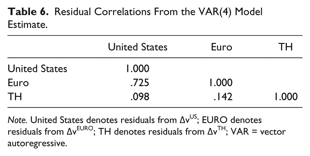
Note. United States denotes residuals from Δv^US; EURO denotes residuals from Δv^EURO; TH denotes residuals from Δv^TH; VAR = vector autoregressive.

The results in Table 6 show that the highest correlation coefficient of .725 is between implied volatilities of the U.S. and Euro stock markets. The correlation coefficient between implied volatilities of the Thai and Euro markets is .142 whereas the correlation coefficient between implied volatilities of the Thai and U.S. market is .098. The latter two coefficients are quite low. The results are consistent with the results of Granger Causality Test, which suggest that the U.S. stock market is influential in transmitting implied volatilities to the other two stock markets. Therefore, it can be argued that the high correlation exhibits the existence of causality while the low correlation exhibits the absence of causality. In other words, causality is justified by the size of the residual correlation.

The results of impulse response analysis are shown in Figure 2. The figure shows the impulse response functions and the Monte Carlo simulated at 95% intervals.

Figure 2.

Impulse responses of implied volatility changes.

The responses of the implied volatility of the Euro stock market to a shock in the implied volatility of the U.S. stock market show that the Euro volatility increases on the next day following the contemporaneous effect of that shock. This impact starts to decay, and the whole impact is incorporated within 3 days. Thereafter, there is a negative impact that lasts for another 2 days. The response of the implied volatility of the Thai stock market to a shock in implied volatility of the U.S. stock market is similar but with lower degree of response and fewer days. Finally, the responses of the U.S.-implied volatility to shocks in the implied volatilities of the Euro and Thai markets are incorporated within 1 day. These findings show that the U.S.-implied volatility leads the other two implied volatilities.

Variance decompositions that are used to ascertain how important the innovations of other variables are in explaining the fraction of each variable at different step ahead forecast variances are presented in Figure 3. The numerical illustration of variance decompositions can also be seen in the appendix table.

Figure 3.

Variance decompositions of changes in implied volatilities.

In Figure 3, the dashed lines represent the Monte Carlo simulated at 95% confidence intervals. The results provide evidence for the independency of the implied volatility of the U.S. stock market because its forecast variance is only caused by its own innovations. Furthermore, the implied volatility of the U.S. market has a significant impact on the Euro-implied volatility, but has no impact on the Thai-implied volatility. Finally, the Euro-implied volatility has no impact on the Thai-implied volatility.

The results clearly show that the U.S. stock market is influential in transmitting volatility as a measure of uncertainty to the Euro and Thai stock markets. However, the Thai stock market is not dependent on the Euro stock market. It should be noted that the period of investigation is the period after subprime crisis. Therefore, the linkages between implied volatility indexes are not strengthened by financial shocks as evidenced by the results of Peng and Ng (2012) and Siriopoulos and Fassas (2013).

Based on the results of the present study, some points are worth discussing. The inter-linkages of volatility expectations can be unsurprisingly observed in international stock markets. The participants in international trading of index options worldwide are foreign investors, such as mutual and pension funds, which are institutional investors. Even though the number of traders is limited, the surge in international portfolio investment has occurred recently due to more open stock markets. International fund managers have played an important role in international stock markets. Also, there is evidence indicating that foreign investors are better informed compared with local investors (Ahn, Kang, & Ryu, 2008). Therefore, the linkages in their expectations have become more apparent. Because the U.S.-implied volatility could dominate other stock markets, portfolio diversification strategy should be taken into account of uncertainty or risk in the U.S. stock market that can transmit to other stock markets. The implied volatility indices also constitute publicly available information for investors. As stated by Siriopoulos and Fassas (2012), implied volatility index contains information about future realized volatility beyond that contained past volatility. Therefore, implied volatility index can be used as an underlying asset in a derivative market. The risk factors that can gauge the expectations of institutional investors are important to the key players in international stock markets. Given the dominance of institutional traders in the international derivative markets, the implied volatilities should reflect international traders’ sentiment.

As for other stock markets, Padhi (2011) finds evidence indicating that the U.S.-implied volatility index imposes a strong impact on those of the Asian- and European-implied volatility indices. However, the Indian-implied volatility index is not affected by the U.S.- and other-implied volatility indices. The reason is that the Indian stock market is lagged in terms of integration with the global financial system. In the case of Thailand, the stock market should not be lagged in terms of integration even though its implied volatility is marginally affected by the U.S.-implied volatility. Implied volatility in level usually contains idiosyncratic risk, especially country specific risk (Poon & Granger, 2003). The present study used changes in implied volatility to reduce this bias. Therefore, the results should be sound. The findings in the present article give recent knowledge for portfolio managers because they need to know the degree of dependency across stock markets so that they can diversify more efficiently.

Concluding Remarks

This study uses the Standard Granger Causality Test and the VAR(4) models to examine implied volatility indices of the U.S., Euro, and Thai stock markets. The empirical results from analyzing the daily data from November 2010 to December 2013 indicate the following: (a) the VAR(4) model used fits the data generally well; (b) there is implied volatility transmissions from the U.S. stock market to the Euro and Thai stock markets, but not the other way around; and (c) the Euro stock market does not influence the Thai stock market in terms of implied volatility spillover. The results have important implication for portfolio mangers operating in the international stock markets in that they can improve their portfolio performance by taking into account the dependencies between implied volatility indices across emerging and advanced stock markets.

Even though the methodology used in this study is not new to the literature, empirical studies that used this methodology in emerging stock markets are few. Therefore, the scope of future work focusing on emerging stock markets should rely on the analysis of implied volatility index instead of the analysis of the volatility generated from various volatility models to examine volatility transmissions among stock markets.

Footnotes

Appendix

Variance Decompositions With SEs.

Period	SE	US_V	Euro_V	TH_V
Panel A: Variance decompositions of US_V
1	0.01724	100.000	0.000	0.000
		(0.000)	(0.000)	(0.000)
2	0.01745	99.619	0.157	0.224
		(0.499)	(0.292)	(0.422)
3	0.01756	99.466	0.221	0.313
		(0.592)	(0.368)	(0.479)
4	0.01789	98.873	0.231	0.896
		(0.955)	(0.415)	(0.863)
5	0.01796	98.804	0.299	0.896
		(1.001)	(0.469)	(0.892)
6	0.01802	98.777	0.323	0.899
		(1.025)	(0.490)	(0.907)
7	0.01804	98.752	0.323	0.925
		(1.045)	(0.490)	(0.927)
8	0.01804	98.741	0.328	0.931
		(1.054)	(0.498)	(0.931)
9	0.01805	98.730	0.335	0.935
		(1.063)	(0.507)	(0.935)
10	0.01806	98.728	0.335	0.937
		(1.064)	(0.507)	(0.937)
Panel B: Variance decompositions of Euro_V
1	0.01791	52.608	47.392	0.000
		(2.885)	(2.885)	(0.000)
2	0.01848	52.444	47.427	0.129
		(2.840)	(2.832)	(0.308)
3	0.01877	52.895	46.856	0.249
		(2.857)	(2.874)	(0.381)
4	0.01895	53.106	46.445	0.448
		(2.812)	(2.875)	(0.630)
5	0.01914	53.594	45.649	0.758
		(2.805)	(2.768)	(0.744)
6	0.01915	53.563	45.610	0.828
		(2.814)	(2.776)	(0.815)
7	0.01920	53.802	45.352	0.846
		(2.822)	(2.779)	(0.835)
8	0.01921	53.834	45.318	0.848
		(2.829)	(2.782)	(0.838)
9	0.01921	53.828	45.323	0.848
		(2.828)	(2.782)	(0.839)
10	0.01922	53.841	45.305	0.853
		(2.831)	(2.785)	(0.843)
Panel C: Variance decompositions of TH_V
1	0.02698	0.968	1.057	97.975
		(0.953)	(0.744)	(1.183)
2	0.0295	1.140	1.041	97.818
		(0.816)	(0.832)	(1.123)
3	0.0298	2.071	1.074	96.855
		(1.273)	(0.839)	(1.487)
4	0.0298	2.136	1.141	96.723
		(1.403)	(0.930)	(1.629)
5	0.0298	2.130	1.298	96.572
		(1.400)	(1.030)	(1.674)
6	0.0299	2.129	1.298	96.574
		(1.412)	(1.051)	(1.699)
7	0.0299	2.140	1.305	96.555
		(1.045)	(1.058)	(1.718)
8	0.0299	2.149	1.305	96.546
		(1.423)	(1.062)	(1.728)
9	0.0299	2.150	1.305	96.545
		(1.426)	(1.063)	(1.728)
10	0.0299	2.150	1.305	96.544
		(1.427)	(1.066)	(1.729)

Note. Cholesky ordering: US_V, Euro_V, and TH_V. SE: Monte Carlo (100 repetitions).

Declaration of Conflicting Interests

The author(s) declared no potential conflicts of interest with respect to the research, authorship, and/or publication of this article.

Funding

The author(s) received no financial support for the research and/or authorship of this article.

Author Biographies

Supachok Thakolsri is currently economic analyst at Ministry of Finance, Bangkok, Thailand. He received PhD degree from National Institute of Development Administration, Bangkok Thailand.

Yuthana Sethapramote received PhD degree from University of Warwick, United Kingdom. He is currently assistant professor of economics, National Institute of Development Administration, Bangkok, Thailand.

Komain Jiranyakul received PhD degree from Texas A&M University, USA. He is currently associate professor of economics, National Institute of Development Administration, Bangkok, Thailand.

References

Ahn

H.-J.

Kang

Ryu

(2008). Informed trading in the index option market: The case of KOSPI200. Journal of Futures Markets, 28, 1118-1146.

Äijö

(2008). Implied volatility term structure linkages between VDAX, VSMI and VSOXX volatility indices. Global Finance Journal, 18, 290-302.

Badshah

I. U.

(2013). Quantile regression analysis of the asymmetric return-volatility relation. Journal of Futures Markets, 33, 235-265.

Black

Sholes

(1973). The pricing of options and corporate liabilities. Journal of Political Economy, 81, 637-654.

Blair

Poon

S. H.

Taylor

(2001). Forecasting S&P100 volatility: The incremental information content of implied volatilities and high frequency index returns. Journal of Econometrics, 105, 5-27.

Bollerslev

Zhou

(2006). Volatility puzzles: A simple framework for gauging return-volatility transmissions. Journal of Econometrics, 131, 123-160.

Chiang

T. C.

Jeon

B. N.

(2007). Dynamic correlation analysis of financial contagion: Evidence from Asian markets. Journal of International Money and Finance, 26, 1206-1228.

Christensen

B. J.

Prabhala

N. R.

(1998). The relation between implied and realized volatility. Journal of Financial Economics, 50, 125-150.

Fleming

Ostdiek

Whaley

(1995). Predicting stock market volatility: A new measure. Journal of Futures Markets, 15, 265-302.

10.

Giot

(2005). Relationships between implied volatility indexes and stock index returns. Journal of Portfolio Management, 31, 92-100.

11.

Granger

C. W. J.

(1969). Investigating causal relationships by econometric models and cross-spectral analysis. Econometrica, 37, 424-438.

12.

Hull

J. C.

(1997). Options, futures and other derivatives. Upper Saddle River, NJ: Prentice Hall.

13.

Kenourgios

(2014). On financial contagion and implied market volatility. International Review of Financial Analysis, 34, 21-30.

14.

Liu

Y. A.

Pan

M. S.

(1997). Mean and volatility spillover effects in the US and Pacific-Basin stock market. Multinational Finance Journal, 1, 47-62.

15.

Nikkinen

Sahlström

(2004). International transmission of uncertainty implicit in stock index option prices. Global Finance Journal, 15, 1-15.

16.

Padhi

(2011, November). On the linkages among selected Asian, European and the US implied volatility indices (NES Working Paper No. 3/2011). India: National Stock Exchange of India Limited.

17.

Peng

W. L.

(2012). Analysing financial contagion and asymmetric market dependence with volatility indices via copulas. Annals of Finance, 8, 49-74.

18.

Poon

S. H.

Granger

C. W. J.

(2003). Forecasting volatility in financial markets: A review. Journal of Economic Literature, 41, 478-539.

19.

Raj

Dhal

(2008). Integration of India’s stock market with global and major regional markets (BIS Papers No. 42). Hong Kong: Bank of International Settlement.

20.

Sim

(1980). Macroeconomics and reality. Econometica, 48, 1-48.

21.

Siriopoulos

Fassas

(2012). An investor sentiment barometer—Greek Implied Volatility Index (GRIV). Global Finance Journal, 23, 77-93.

22.