On the Temporal Causal Relationship Between Macroeconomic Variables

Abstract

The present study examines the dynamic interactions among macroeconomic variables such as real output, prices, money supply, interest rate (IR), and exchange rate (EXR) in India during the pre-economic crisis and economic crisis periods, using the autoregressive distributed lag (ARDL) bounds test for cointegration, Johansen and Juselius multivariate cointegration test, Granger causality/Block exogeneity Wald test based on Vector Error Correction Model, variance decomposition analysis and impulse response functions. The empirical results reveal a stronger long-run bilateral relationship between real output, price level, IR, and EXR during the pre-crisis sample period. Moreover, the empirical results confirm a unidirectional short-run causality running from price level to EXR, IR to price level, and real output to money supply during the pre-crisis period. Also, it is evident from the test results that there exist short-run bidirectional relationships running between real output and EXR, price level and IR, and IR and EXR in the pre-crisis era, respectively. Most importantly, long-run bidirectional causality is found between real output, EXR, and IR during the economic crisis period. And the study results indicate short-run bidirectional causality between money supply and EXR, IR and price level, and IR and output in India during the crisis era. Also, a short-run unidirectional causality runs from prices to real output in the crisis period.

Introduction

The relationship among money supply, income, and prices has long been a subject of controversy between the Keynesian and monetarist schools of thought. Different schools of economic thought have postulated various theories on relationships between macroeconomic variables. The classical school explained that a change in prices is basically due to changes in money supply. However, Keynesians criticized and rejected the proportionality between money supply and prices due to its instability in explaining the causes and remedies for the great economic debacle like Great Depression of 1930s. The Keynesians held the view that money does not play an active role in changing income and prices nor does it causes instability in the economy. They postulated that changes in income causes changes in money stock via demand for money implying that the direction of causation runs from income to money, not vice versa. Monetarists, on the contrary, argued that money plays an active role and leads to the changes in income and prices. There is unidirectional causation that runs from money to income and prices. Moreover, Fischer (1962) claimed the possibility of reverse causation and concluded that there is mutual interaction between money and other macrovariables. M. Friedman and Schwartz (1963) also supported this argument by stating that though the influence of money to economic activity is predominant, there is also the possibility of influences running the other way (at least in the short run). The Banking school also supported the reverse causation between money and income, thereby arguing for endogeneity of money supply (Froyen, 2004).

As a consequence of conflicting theoretical debate, the relationship has been extensively investigated in empirical literature by researchers for both developed and developing countries over different sample periods and provided the conflicting evidences on this issue. Examples include Ramachandra (1986), Miller (1991), B. Friedman and Kuttner (1992), Ramachandran and Kamaiah (1992), Stock and Watson (1993), Boucher and Flynn (1996), Brahmananda and Nagaraju (2003), Ramachandran (2004), Jamie (2005), Herwartz and Reimers (2006), Majid (2007), Saatcioglu and Korap (2008), Jiranyakul (2009), Rami (2010), Maitra (2011), Hossain (2011), Yadav and Lagesh (2011), Shams (2012), and Bilquees, Mukhtar, & Sohail (2012).

One of the most important objectives of macroeconomic policy modeling is to achieve sustained output growth. Formation of effective macroeconomic policy requires examination of underlying relationship among the policy variables. The growing complexities of monetary management, in the context of recent global economic crisis, required that the process of policy formulation should be based on a wider range of macroeconomic variables. The transmission of the global financial crisis to India has clearly demonstrated that the country has become integrated into the global business cycle. Although the Indian economy experienced acceleration in growth in the early 2000s, with India’s increased linkage with the world economy, India could not be expected to remain immune to the recent ongoing global economic crisis. The knock-on effect of the financial crisis was felt in all the sectors of the economy and this created disturbances in the macroeconomic environment of Indian economy. This include fluctuations in money supply, increase in price level, accelerating inflation, instability in exchange rate (EXR), and affecting the aggregate output of the economy. Before the economic crisis of 2008, India recorded an average GDP growth of 8% per annum during 2003-2007, but on the onset of global crisis with the adverse impact of demand shocks, the economic growth fell from 9.2% in 2007-2008 to 6.7% and 6.5% in 2008-2009 and 2010-2011, respectively. This has significantly affected the macroeconomic relationship of monetary and real sector variables. The adverse impact of the global financial crisis was mitigated by a series of proactive policy measures. While India’s monetary policy largely aimed at enhancing domestic liquidity, which had shrunk considerably since the collapse of the U.S. investment bank, Lehman Brothers, its fiscal policy sought to boost aggregate demand. A number of policy measures were also initiated to attract foreign capital back into the country. All these measures were able to curb the decline in the growth rate to a certain extent, and there have been several signs of an incipient recovery since April 2009. However, they have also raised a number of policy challenges for the medium term. Overall, the mounting macroeconomic instability in India in recent years, characterized by high rates of inflation, a fragile foreign exchange position, high rates of interest, increases uncertainty for any investor or producer and slowing down economic growth makes imperative to understand the temporal causal nexus between macroeconomic variables in the Indian context by allowing us to look into what happens at different periods of interest, that is, pre and crisis era, respectively. It is worth emphasizing that the empirical issue of money, price, output, EXR, and interest rate (IR) relationships is of crucial importance to the Indian economy, given the current economic environment. The present study assumes greater significance for effective implementation of its monetary policy and achieves the desired target of growth keeping stability of prices and EXRs. Furthermore, since global economic crisis of 2008, no study exists in India that had examined the causal directions among macroeconomic variables in the context of recent ongoing global economic crisis. In this article, we attempt to investigate the causal nexus between money, income, price, IR, and the EXRs in India during pre-global economic crisis and crisis era.

The remainder of our article is organized as follows. “Method” section presents methodology and data of the study. The empirical results and discussion are provided in “Empirical Results” section and “Conclusion” section presents concluding remarks.

Method

Autoregressive Distributed Lag (ARDL) Bounds Testing Approach to Cointegration

The ARDL bounds testing approach was used to investigate the long-run equilibrium relationship among the selected macroeconomic variables in India during the pre-crisis period. The ARDL modeling approach was originally introduced by Pesaran and Shin (1999) and further extended by Pesaran, Shin, and Smith (2001). This approach estimates the short- and long-run components of the model simultaneously, removing problems associated with omitted variables and autocorrelation. Besides, the standard Wald or F statistics used in the bounds test has a non-standard distribution under the null hypothesis of no-cointegration relationship between the examined variables, irrespective of whether the underlying variables are I(0), I(1), or fractionally integrated. Moreover, once the orders of the lags in the ARDL model have been appropriately selected, we can estimate the cointegration relationship using a simple Ordinary Least Square (OLS) method. The ARDL-unrestricted error correction model (UECM) used in the present study has the following form as expressed in Equation 1:

$$\Delta \text{In}{Y}_1={\beta }_0+{\displaystyle \sum _{i=1}^m{\delta }_1\Delta \text{In}{Y}_{2t-i}}+{\displaystyle \sum _{i=1}^n{\delta }_2\Delta \text{In}{Y}_{3t-i}}+{\displaystyle \sum _{i=1}^p{\delta }_3\Delta \text{In}{Y}_{4t-i}}+{\displaystyle \sum _{i=1}^q{\delta }_4\Delta \text{In}{Y}_{5t-i}}+{\displaystyle \sum _{i=1}^r{\delta }_5\Delta \text{In}{Y}_{1t-i}}+{\beta }_1\text{In}{Y}_{1t-i}+{\beta }_2\text{In}{Y}_{2t-i}+{\beta }_3\text{In}{Y}_{3t-i}+{\beta }_4\text{In}{Y}_{4t-i}+{\beta }_5\text{In}{Y}_{5t-i}+{\epsilon }_t,$$

$$\Delta \text{In}{Y}_2={\beta }_0+{\displaystyle \sum _{i=1}^m{\delta }_1\Delta \text{In}{Y}_{1t-i}}+{\displaystyle \sum _{i=1}^n{\delta }_2\Delta \text{In}{Y}_{3t-i}}+{\displaystyle \sum _{i=1}^p{\delta }_3\Delta \text{In}{Y}_{4t-i}}+{\displaystyle \sum _{i=1}^q{\delta }_4\Delta \text{In}{Y}_{5t-i}}+{\displaystyle \sum _{i=1}^r{\delta }_5\Delta \text{In}{Y}_{2t-i}}+{\beta }_1\text{In}{Y}_{1t-i}+{\beta }_2\text{In}{Y}_{3t-i}+{\beta }_3\text{In}{Y}_{4t-i}+{\beta }_4\text{In}{Y}_{5t-i}+{\beta }_5\text{In}{Y}_{2t-i}+{\epsilon }_t,$$

$$\Delta \text{In}{Y}_3={\beta }_0+{\displaystyle \sum _{i=1}^m{\delta }_1\Delta \text{In}{Y}_{1t-i}}+{\displaystyle \sum _{i=1}^n{\delta }_2\Delta \text{In}{Y}_{2t-i}}+{\displaystyle \sum _{i=1}^p{\delta }_3\Delta \text{In}{Y}_{4t-i}}+{\displaystyle \sum _{i=1}^q{\delta }_4\Delta \text{In}{Y}_{5t-i}}+{\displaystyle \sum _{i=1}^r{\delta }_5\Delta \text{In}{Y}_{3t-i}}+{\beta }_1\text{In}{Y}_{1t-i}+{\beta }_2\text{In}{Y}_{2t-i}+{\beta }_3\text{In}{Y}_{4t-i}+{\beta }_4\text{In}{Y}_{5t-i}+{\beta }_5\text{In}{Y}_{3t-i}+{\epsilon }_t,$$

$$\Delta \text{In}{Y}_4={\beta }_0+{\displaystyle \sum _{i=1}^m{\delta }_1\Delta \text{In}{Y}_{1t-i}}+{\displaystyle \sum _{i=1}^n{\delta }_2\Delta \text{In}{Y}_{2t-i}}+{\displaystyle \sum _{i=1}^p{\delta }_3\Delta \text{In}{Y}_{3t-i}}+{\displaystyle \sum _{i=1}^q{\delta }_4\Delta \text{In}{Y}_{5t-i}}+{\displaystyle \sum _{i=1}^r{\delta }_5\Delta \text{In}{Y}_{4t-i}}+{\beta }_1\text{In}{Y}_{1t-i}+{\beta }_2\text{In}{Y}_{2t-i}+{\beta }_3\text{In}{Y}_{3t-i}+{\beta }_4\text{In}{Y}_{5t-i}+{\beta }_5\text{In}{Y}_{4t-i}+{\epsilon }_t,$$

$$\Delta \text{In}{Y}_5={\beta }_0+{\displaystyle \sum _{i=1}^m{\delta }_1\Delta \text{In}{Y}_{1t-i}}+{\displaystyle \sum _{i=1}^n{\delta }_2\Delta \text{In}{Y}_{2t-i}}+{\displaystyle \sum _{i=1}^p{\delta }_3\Delta \text{In}{Y}_{3t-i}}+{\displaystyle \sum _{i=1}^q{\delta }_4\Delta \text{In}{Y}_{4t-i}}+{\displaystyle \sum _{i=1}^r{\delta }_5\Delta \text{In}{Y}_{5t-i}}+{\beta }_1\text{In}{Y}_{1t-i}+{\beta }_2\text{In}{Y}_{2t-i}+{\beta }_3\text{In}{Y}_{3t-i}+{\beta }_4\text{In}{Y}_{4t-i}+{\beta }_5\text{In}{Y}_{5t-i}+{\epsilon }_t,$$

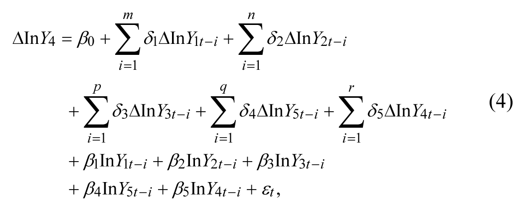
where Y₁, Y₂, Y₃, Y₄, and Y₅ represent selected macroeconomic variables for the study such as EXR, money supply (M3), price level (consumer price index [CPI]), index of industrial production (IIP), and IR, respectively. t is the time dimension, Δ denotes a first difference operator, β₀ is an intercept, and ε _t is a white noise error term.

The first step in the ARDL bounds testing approach is to estimate Equations 1-5 using OLS method to test for existence of a long-run relationship among the variables by conducting an F test for the joint significance of the coefficients of the lagged level variables, that is, H₀: β₁= β₂= β₃= β₄= β₅ = 0 against the alternative, H₁: β₁ ≠ β₂ ≠ β₃ ≠ β₄ ≠ β₅ ≠ 0, which normalize on Y₁ by F(Y₁/Y₂, Y₃, Y₄, Y₅). Two sets of critical value bounds for the F statistic are generated by Pesaran et al. (2001). If the computed F statistic falls below the lower bound critical value, the null hypothesis of no cointegration cannot be rejected. On the contrary, if the computed F statistic lies above the upper bound critical value; the null hypothesis is rejected, implying that there is a long-run cointegration relationship among the variables in the model. Nevertheless, if the calculated value falls within the bounds, inference is inconclusive. Similar testing procedure was followed to calculate the F statistic when each of Y₂, Y₃, Y₄, and Y₅ appear as a dependent variable and other variables are considered as explanatory variables in the specification.

Johansen and Juselius (1990) Multivariate Cointegration Approach

Johansen and Juselius (1990) multivariate cointegration approach was used to investigate the long-run equilibrium relationship among the selected macroeconomic variables in India during the crisis period. Before doing cointegration analysis, it is necessary to test the stationary of the series. The Augmented Dickey–Fuller (ADF; Dickey & Fuller, 1979) and Phillips–Perron (PP; Phillips & Perron, 1988) tests were used to infer the stationary of the series. If the series are non-stationary in levels and stationary in differences, then there is a chance of cointegration relationship between them, which reveals the long-run relationship between the series. Johansen’s cointegration test has been used to investigate the long-run relationship between the variables. Besides, the causal nexus between selected macroeconomic variables was investigated by estimating the following Vector Error Correction Model (VECM; Johansen, 1988; Johansen & Juselius, 1990):

$$\Delta Y_t=\mu +{\Gamma }_i\Delta Y_{t-i}+\cdots +{\Gamma }_{k-1}\Delta Y_{t-k+1}+\Pi Y_{t-1}+{\epsilon }_t,$$

where ΔY_t is (n × 1) vector of macroeconomic variables such as money, income, price, IR, and the EXRs in period t, µ is (n × 1) vector of constant terms, Γ _i (i = 1, . . . k − 1) represents the (n × n) coefficient matrix of short-run dynamics, Π is the n × n long-term impact matrix, and ε_1t is (n × 1) vector of error term, and it is independent from all explanatory variables. When cointegration is present, we can decompose the long-term response matrix into A = αβ′, where α and β are n × r matrices. In other words, the expression β′ Y_t−1 defines the stationary linear combinations (cointegration relations) of the I(1) vector Y_t, while the matrix α of the error correction terms (ECTs) describe how the system variables adjust to the equilibrium error from the previous period, β′ Y_t−1.

The Johansen’s cointegration proposed two test statistics through Vector Autoregressive (VAR) model that are used to identify the number of cointegrating vectors, namely the trace test statistic and the maximum eigenvalue test statistic. These test statistics can be constructed as,

$${\lambda }_{\text{trace}}\left(r\right)=-T{\displaystyle \sum _{i=r+1}^n\text{ln}\left(1-{\stackrel{⌢}{\lambda }}_i\right)},$$

$${\lambda }_{\text{max}}\left(r,r+1\right)=-T\text{ln}\left(1-{\stackrel{⌢}{\lambda }}_{r+i}\right),$$

where ${\stackrel{⌢}{\lambda }}_i$ are the eigenvalues obtained from the estimate of the A_k matrix and T is the number of usable observations. The λ_trace tests the null that there are at most r cointegrating vectors, against the alternative that the number of cointegrating vectors is greater than r and the λ_max tests the null that the number of cointegrating vectors is r, against the alternative of r + 1. Critical values for the λ_trace and λ_max statistics are provided by MacKinnon–Haug–Michelis (MacKinnon, Haug, & Michelis, 1999).

Vector Error Correction Granger Causality

The VECM was used to investigate the temporal causality between selected macroeconomic variables in India during the pre-crisis and crisis period. The Granger Representation Theorem (Engle & Granger, 1987) states that if a set of variables is cointegrated, then there exists a valid error correction representation of the data, in which the short-term dynamics of the variables in this system are influenced by the deviation from long-term equilibrium. In a VECM, short-term causal effects are indicated by changes in other differenced explanatory variables (i.e., the lagged dynamic terms in Equation 6). The long-term relationship is implied by the level of disequilibrium in the cointegration relationship, that is, the lagged ECT. Thus, in the cointegration model, the proposition of “Y_k not Granger causing Y_l” in the long-term is equivalent to α _kl = 0. Y_l is said to be weakly exogenous for parameter β, that is, Y_l does not react to equilibrium errors. Besides, the proposition “Y_k do not Granger-cause Y_l” in the short term is equivalent to Γ _kl (L) = 0, where L is the lag operator. Hence, the VECM is useful for detecting short- and long-term Granger causality tests (Granger, 1969). The VECM corresponding to Equation 1 can be formulated as follows:

$$\Delta Y_{1t}{\text{=µ}}_1+{\text{γ}}_1{z}_{t-1}+{\displaystyle \sum _{i=1}^{p-1}{\text{θ}}_{1i}\Delta Y_{1t-i}}+{\displaystyle \sum _{i=1}^{p-1}{\text{δ}}_{1i}\Delta Y_{2t-i}}+{\displaystyle \sum _{i=1}^{p-1}{\text{ξ}}_{1i}\Delta Y_{3t-i}}+{\displaystyle \sum _{i=1}^{p-1}{\mho }_{1i}\Delta Y_{4t-i}}+{\displaystyle \sum _{i=1}^{p-1}{\text{λ}}_{1i}\Delta Y_{5t-i}}+{\text{ε}}_{1t},$$

$$\Delta Y_{2t}{\text{=µ}}_2+{\text{γ}}_2{z}_{t-1}+{\displaystyle \sum _{i=1}^{p-1}{\text{δ}}_{2i}\Delta Y_{2t-i}}+{\displaystyle \sum _{i=1}^{p-1}{\text{θ}}_{2i}\Delta Y_{1t-i}}+{\displaystyle \sum _{i=1}^{p-1}{\text{ξ}}_{2i}\Delta Y_{3t-i}}+{\displaystyle \sum _{i=1}^{p-1}{\mho }_{2i}\Delta Y_{4t-i}}+{\displaystyle \sum _{i=1}^{p-1}{\text{λ}}_{2i}\Delta Y_{5t-i}}+{\text{ε}}_{1t},$$

$$\Delta Y_{3t}{\text{=µ}}_3+{\text{γ}}_3{z}_{t-1}+{\displaystyle \sum _{i=1}^{p-1}{\text{ξ}}_{3i}\Delta Y_{3t-i}}+{\displaystyle \sum _{i=1}^{p-1}{\text{θ}}_{3i}\Delta Y_{1t-i}}+{\displaystyle \sum _{i=1}^{p-1}{\text{δ}}_{3i}\Delta Y_{2t-i}}+{\displaystyle \sum _{i=1}^{p-1}{\mho }_{3i}\Delta Y_{4t-i}}+{\displaystyle \sum _{i=1}^{p-1}{\text{λ}}_{3i}\Delta Y_{5t-i}}+{\text{ε}}_{1t},$$

$$\Delta Y_{4t}{\text{=µ}}_4+{\text{γ}}_4{z}_{t-1}+{\displaystyle \sum _{i=1}^{p-1}{\mho }_{4i}\Delta Y_{4t-i}}+{\displaystyle \sum _{i=1}^{p-1}{\text{θ}}_{4i}\Delta Y_{1t-i}}+{\displaystyle \sum _{i=1}^{p-1}{\text{δ}}_{4i}\Delta Y_{2t-i}}+{\displaystyle \sum _{i=1}^{p-1}{\text{ξ}}_{4i}\Delta Y_{3t-i}}+{\displaystyle \sum _{i=1}^{p-1}{\text{λ}}_{4i}\Delta Y_{5t-i}}+{\text{ε}}_{1t},$$

$$\Delta Y_{5t}={\text{µ}}_5+{\text{γ}}_5{z}_{t-1}+{\displaystyle \sum _{i=1}^{p-1}{\text{λ}}_{5i}\Delta Y_{5t-i}}+{\displaystyle \sum _{i=1}^{p-1}{\text{θ}}_{5i}\Delta Y_{1t-i}}+{\displaystyle \sum _{i=1}^{p-1}{\text{δ}}_{5i}\Delta Y_{2t-i}}+{\displaystyle \sum _{i=1}^{p-1}{\text{ξ}}_{5i}\Delta Y_{3t-i}}+{\displaystyle \sum _{i=1}^{p-1}{\mho }_{5i}\Delta Y_{4t-i}}+{\text{ε}}_{1t},$$

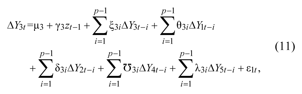
where γ’_sz_t−1 is the ECT derived from the cointegrating vector. θ, δ, ξ, Ʊ, and λ are the short-run parameters to be estimated, p is the lag length, and ε _t are assumed to be stationary random processes with a mean of zero and constant variance.

For each equation in the VECM, we use short-term Granger causality to test whether endogenous variables can be treated as exogenous by the joint significance of the coefficients of each of the other lagged endogenous variables in that equation. The short-term significance of sum of the each lagged explanatory variables (θ’s, δ’s, ξ’s, Ʊ’s, and λ’s) can be exposed either through joint F or Wald χ² test. Besides, the long-term causality is implied by the significance of the t tests of the lagged ECT (ECT_t−1). However, the non-significance of both the t statistics and joint F or Wald χ² tests in the VECM indicates econometric exogeneity of the dependent variable.

Variance Decomposition Analysis (VDA) and Impulse Response Function (IRF)

Finally, the study used VDA and IRFs to assess to what extent shocks to certain macroeconomic variables are explained by other variables in the system. VDA measures the proportions of forecast error variance in a variable that is explained by innovations (impulses) in it and by the other variables in the system. For example, it explains what proportions of the changes in a particular variable can be attributed to changes in the other lagged explanatory variables. In a statistical sense, if a variable explains most of its own shock, then it does not allow variances of other variables to contribute to it being explained and is therefore said to be relatively exogenous. Impulse response analysis traces out the responsiveness of the dependent variable in VECM to shocks to each of the other explanatory variables over the period of time. A shock to a variable in a VECM framework not only directly affects that variable but also transmits its effect to all other endogenous variables in the system.

The monthly macroeconomic data used in this study consists of IIP, Money Supply (M3), Price (CPI), IR, and nominal EXR from April 1994 to July 2012. The study divides the entire data set into two sample periods, that is, the pre-economic crisis period and economic crisis period. The global financial crisis leads to a severe recession in the country’s real economy. The signs of a recession are evident in the Central Statistical Organization (CSO)’s estimates of growth of real GDP for the last quarter of 2007-2008 and the first quarter of 2008-2009. GDP growth for the first quarter of 2008-2009 slowed down to 7.9%. Global crisis spilled over in India through financial as well as real channels. Because of the limited exposure of Indian banks to distressed assets, India was not directly affected by the financial crisis, but the indirect effects through trade and capital flows were severe. Patnaik and Shah (2010) suggest that since Indian multinationals that were using the global money market were short of dollars after the collapse of Lehman Brothers, they borrowed in India and took capital out of the country, thereby tightening the money market. At this point, the Reserve Bank of India (RBI) reversed its tight monetary policy stance and started injecting liquidity into the economy through a variety of measures, which resulted in a moderation of the call money rates. However, despite these measures, which included lowering policy rates, relaxing provisioning norms and reducing risk weights on exposures, the credit growth rate declined from 30% in October 2008 to less than 17% in March 2009, and to 10% in October 2009. Non-food bank credit declined by nearly 5% in 2008-2009 compared with the previous year, while non-bank resource flows to the commercial sector fell by more than 20%. In particular, there has been a sharp decline in public issues by non-financial entities, and net issuance of commercial paper and net credit by housing finance companies. Indian government in coordination with RBI responded with several policy measures to minimize the impact of the crisis.

In January 2008, the global financial crisis came into existence with sub-prime effect and it spillover into the rest of the world. Subsequently, the European sovereign debt crisis began in early 2010 and worsened the macroeconomic conditions of the Indian economy and significantly affected its economic growth. As discussed above, the Indian economy persistently faced retarded growth momentum and macroeconomic imbalances with high inflationary pressure as a result of enduring global economic crisis. Hence, the study considered the data span from January 2008 to July 2012 as economic crisis period. Whereas the data set prior to the crisis period from April 1994 to December 2007 is considered to be the non-crisis period.

The necessary data on macroeconomic variables are collected from various issues of Handbook of Statistics on Indian Economy, RBI, Mumbai, India. The proxy variable for money supply used is Broad money (M3), which consists of Narrow money, that is, currency with public, other deposits with RBI and demand deposits of banks (M1) plus time deposits. CPI, index for industrial production (IIP), and call money rate have been used as proxy variables for prices, output, and IR, respectively.

Empirical Results

A perquisite for testing cointegration between macroeconomic variables is that all variables are non-stationary. The ADF and PP tests were used to check whether the variables contain a unit root or not. Table 1 reports the results of ADF and PP unit root test for the two sample periods, that is, pre-economic crisis period and economic crisis period. For the pre-crisis period, the table results confirm that variables, prices (CPI), and IR are stationary at levels and are integrated of order I(0), while IIP, money supply (M3), and EXR are integrated of order I(1), that is, they are non-stationary at levels but stationary at first differences. For the economic crisis period, the table result reveals that all the selected macroeconomic variables are found to be stationary at their first differences and are integrated at I(1).

Table 1.

Results of Augmented Dickey–Fuller and Phillip–Perron Unit Root Tests.

	Augmented Dickey–Fuller test statistics		Phillips–Perron test statistics
	Pre-crisis period	Crisis period	Pre-crisis period	Crisis period
Variables	Level	First difference	Level	First difference
EXR	−2.118	−9.210*	−0.171	−6.149*
IIP	0.985	−2.735***	0.784	−2.356**
IR	−5.825*	—	−5.990*	—
CPI	−4.282*	—	−3.983**	—
M3	1.094	−2.765***	−1.305	−3.639*

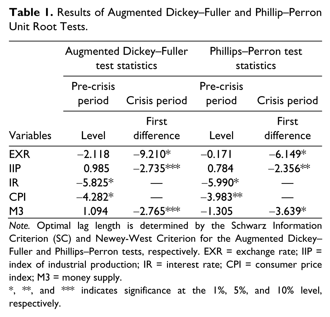
Note. Optimal lag length is determined by the Schwarz Information Criterion (SC) and Newey-West Criterion for the Augmented Dickey–Fuller and Phillips–Perron tests, respectively. EXR = exchange rate; IIP = index of industrial production; IR = interest rate; CPI = consumer price index; M3 = money supply.

*

, **, and *** indicates significance at the 1%, 5%, and 10% level, respectively.

The ARDL bounds test approach and the Johansen and Juselius (1990) multivariate cointegration test was performed to examine the long-run relationship between the macroeconomic variables for the pre-crisis and crisis period, respectively.

Table 2 presents the result of ARDL bounds test approach for cointegration relationship based on Equations 1-5 during the pre-crisis period. The appropriate lag length was selected on the basis of Akaike Information Criterion (AIC) for the conditional ARDL-UECM. The empirical results reveal that calculated F statistic for the Equation 1, that is, F_EXR(EXR/M3, CPI, IIP, IR) is found to be higher than the upper bound critical value at 1% level of significance, indicating there is a stable long-run cointegration relationship between EXR and other selected macroeconomic variables. Similarly, when price level is considered as a dependent variable, the calculated F statistic is found to be statistically significant at 1% level, implying a long-run cointegration relationship among price level and other macroeconomic variables. Besides, the empirical results confirm that money supply, price, and IR share a long-run relationship with real output. Furthermore, there exists a long-run cointegration relation between real output, money supply, price, and EXR when the IR variable is the dependent variable. However, the analysis reveals no cointegrating relationship among money supply and other macroeconomic variables when the regression is normalized on money supply.

Table 2.

ARDL Cointegration Bound Testing Approach for the Pre-Crises Period.

Model specification	F statistics	Inference
FEXR(EXR/M3, CPI, IIP, IR)	5.240 a	Cointegration
FM3(M3/EXR, CPI, IIP, IR)	1.791	No cointegration
FCPI(CPI/EXR, M3, IIP, IR)	6.759 a	Cointegration
FIIP(IIP/EXR, M3, CPI, IR)	12.86 a	Cointegration
FIR(IR/EXR, M3, CPI, IIP)	7.386 a	Cointegration

Note. Asymptotic critical value bounds are obtained from Pesaran, Shin, and Smith (2001), p. 300; Case III: Unrestricted intercept and no trend for k = 5. Lower bound I(0) = 3.416 and upper bound I(1) = 4.681 at 1% significance level. ARDL = autoregressive distributed lag; EXR = exchange rate; M3 = money supply; CPI = consumer price index; IIP = index of industrial production; IR = interest rate.

a

Computed statistic falls above the upper bound value.

For the crisis period, the Johansen and Juselius (1990) multivariate cointegration test was performed to examine the long-run relationship between the selected macroeconomic variables in India and the results are reported in Table 3. Both trace and maximum eigenvalue indicates the presence of two cointegrating vector among the selected macroeconomic variables at 5% significant level, implying that there is a well-defined long-run equilibrium relationship among the variables under consideration.

Table 3.

Johansen Maximum Likelihood Cointegration Test for the Crises Period.

Null hypothesis	Alternative hypothesis	Trace statistics	5% Critical value	Maximum eigen statistics	5% Critical value
H0: r = 0	H1: r = 1	97.36**	69.81	46.90**	33.87
H0: r ≤ 1	H1: r = 2	50.09**	47.85	28.18**	27.58
H0: r ≤ 2	H1: r = 3	21.91	29.79	11.64	21.13
H0: r ≤ 3	H1: r = 4	10.26	15.49	10.19	14.26
H0: r ≤ 4	H1: r = 5	0.075	3.884	0.075	3.841

Note. r is the number of cointegrating vector. Critical values are noted from MacKinnon–Haug–Michelis (MacKinnon, Haug, & Michelis, 1999).

**

denotes the significance at 5% level.

The results of the estimated multivariate VECM for both the sample periods are presented in Table 4. The long-run dynamics was examined through the effect of the lagged ECT in the VECM. For the pre-crisis period, the table results clearly show significant ECTs with expected negative sign for real output, price level, IR, and EXR. This implies that these variables are significantly adjusted to disequilibrium from the long-run relationship or the response with which the previous period’s deviations in real output, price level, IR, and EXR from the long-run equilibrium path are corrected in consequent period. However, the error correction coefficient for the money supply is found to be insignificant, confirming the results obtained under the ARDL bounds test of cointegration that money supply is not related to real output, EXR, price, and IR in the long run. The empirical results reveal that the selected macroeconomic variables, namely real output, price level, IR, and EXR are significantly influenced by each other, suggesting a stronger long-run bilateral relationship between them in the pre-crisis sample period. However, the causality between money supply and real output, price, EXR, and IR is found to be neutral in the long run.

Table 4.

Vector Error Correction Model Estimates.

	ΔEXR	ΔM3	ΔCPI	ΔIIP	ΔIR
Pre-crisis period—April 1994 to December 2007
Constant	−6.28E-05 (−0.062)	9.86E-05 (0.111)	−0.00011 (−0.206)	0.00016 (0.055)	0.00638 (0.217)
ECT(−1)	−0.2543* (−3.357)	0.0824 (1.225)	−0.1217* (−2.800)	−1.5747* (−7.087)	−1.5656*** (−1.713)
Crisis period—January 2008 to July 2012
Constant	−0.00027 (−0.084)	−0.00032 (−0.055)	5.71E-05 (0.122)	0.00045 (0.062)	−0.00035 (−0.030)
ECT(−1)	−0.1645*** (−1.777)	0.2474 (1.434)	0.0155 (1.132)	−1.7794* (−8.399)	−1.7423* (−4.961)

Note. EXR = exchange rate; M3 = money supply; CPI = consumer price index; IIP = index of industrial production; IR = interest rate; ECT = error correction term.

*

and *** denote the significance at 1% and 10% level, respectively.

The coefficients of lagged ECT show the speed of adjustment of disequilibrium in the economic crisis period of study. This implies that the estimated error correction coefficients of EXR, IIP, and IR are negative and statistically significant ensuring that the adjustment process from the short-run deviation is quite slow except EXR. The error correction coefficients for the EXR, real output, and IR are found to have expected negative sign and statistically significant, implying long-run bidirectional causality between EXR, real output, and IR during the crisis period. However, the money supply is found to be neutral and is not influenced by the output, price, EXR, and IR in the long run. Likewise, the price variable is also not influenced by the output, money supply, EXR, and IR in the long run.

Table 5 provides the results of Granger causality/Block exogeneity Wald test based on VECM to identify the short-run causality between the selected macroeconomic variables in India during the pre-crisis and crisis periods. The empirical results for the pre-crisis sample period confirm a unidirectional short-run causality running from price level to EXR, IR to price level, and real output to money supply. Also, it is evident from the test results that there exist short-run bidirectional relationships running between real output and other selected macroeconomic variables, namely EXR, price level, and IR. The feedback relationship is also observed between IR and EXR variables in the short run.

During the economic crisis period, the table results indicate short-run bidirectional causality between money supply and EXR, IR and price level, and IR and output. Also, a short-run unidirectional causality runs from prices to real output in the crisis era.

The results of VDA based on VECM for the selected macroeconomic variables over a 20-month horizon are presented in Appendix A. The VDA result for the pre-crisis period shows that real output variable was 100% explained by its own shock on the first trading day, but it continued to reduce to 59.25% on the 20th month. The shock explained by changes in price variable on real output is only about 30% on the 20th month. Moreover, the results confirm that variables under consideration, namely money supply (86.27%) followed by price level (80.74%), IR (76.88%), and EXR (67.62%) are said to be fairly exogenous variables, as they are explained by itself for its own shock on the 20th month horizon. Furthermore, the EXR accounts for 28.33% of the shock explained by real output in the long run.

Similarly, the findings of VDA for the economic crisis period reveal that selected macroeconomic variables are mainly explained by its own shock in the system. The forecast error variance of real output is mainly explained by price level (15.88%) and EXR (14.98) in the long run. Besides, the real output is the most important variable in explaining the variation in the EXR and IR in the long run.

The IRFs in Appendix B (Figures B1 and B2) illustrates the responses of the endogenous variables to an initial shock of one standard deviation in real output, price level, money supply, IR, and EXR. The IRFs in Appendix Figure B1 for the pre-crisis sample period clearly show that the real output has immediate positive response to a one-standard-deviation shock in price level and the response tend to be stable in the long run. The EXR explains immediate effect to a one-standard-deviation shock in real output throughout the long-run horizon. Responses to one standard deviation in EXR to price tend to be small and stabilized over the time period. The IRFs in Appendix Figure B2 for the economic crisis period shows that real output has moderate response to a one-standard-deviation shock in price level and EXR throughout the 20-month horizon. Besides, the response to a one-standard-deviation shock in EXR and IR to price variable tend to be stable in the long run. By and large, the IRFs for both the sample periods appear to be consistent with the results obtained from the VDA discussed above.

Conclusion

This study examines the dynamic interactions among macroeconomic variables such as real output, prices, money supply, IR, and EXR in India during the pre-economic crisis and economic crisis periods, using the ARDL bounds test for cointegration, Johansen and Juselius (1990) multivariate cointegration test, Granger causality/Block exogeneity Wald test based on VECM, VDA, and IRFs. The study uses monthly data over the period from April 1994 to July 2012 and the entire data set has been divided into two sample periods, that is, the pre-economic crisis period (April 1994 to December 2007) and economic crisis period (January 2008 to July 2012).

For the pre-economic crisis period, the ARDL bound test approach indicates a stable long-run cointegration relationship between selected macroeconomic variables under consideration. However, the analysis reveals no cointegrating relationship among money supply and other macroeconomic variables when the regression is normalized on money supply. The empirical results reveal a stronger long-run bilateral relationship between real output, price level, IR, and EXR in the pre-crisis sample period. While the causality between money supply and other macroeconomic variables, namely real output, price, EXR, and IR are found to be neutral in the long run.

Moreover, the empirical results confirm a unidirectional short-run causality running from price level to EXR, IR to price level, and real output to money supply during the pre-crisis sample period. Also, it is evident from the test results that there exist short-run bidirectional relationships running between real output and other selected macroeconomic variables, namely EXR, price level, and IR in the pre-crisis era. The feedback relationship is also observed between IR and EXR variables in the short run.

During the economic crisis period, the cointegration test results confirm a well-defined long-run equilibrium relationship among the macroeconomic variables, namely real output, money supply, prices, EXR, and IR. The long-run bidirectional causality is observed between real output, EXR, and IR during the economic crisis era. Furthermore, the money supply and real output are found to be neutral in the long run. The study results indicate short-run bidirectional causality between money supply and EXR, IR and price level, and IR and output in the economic crisis period. Also, a short-run unidirectional causality runs from prices to real output in the crisis period.

To conclude, our study does not support monetarists’ view for the both sample periods. Alternatively, during the pre-crisis sample period, the study findings support the Keynesian view that changes in income lead to changes in the stock of money through the demand for money in the short run. Therefore, the direction of causation runs from income to money without any feedback. In addition, changes in price level influences the changes in EXR, and changes in IR causes the changes in price level in the short run during the pre-crisis era. Most importantly, our study shows that prices cause real output in the short run during the economic crisis period. The study evidences suggest that the RBI has to concentrate on the price level as its central target variable of its monetary policy is to achieve macroeconomic stability and promote economic activities in the current economic crisis scenario.