Sage Journals: Discover world-class research

Abstract

Given that political events have substantial effect on new economic policies and economic performance of the country, this article aims to examine the behavior of the investors’ sentiment in terms of implied volatility index trailed by the U.S. presidential elections. The study empirically tests whether the presidential elections in 2012/2016 do contain the important market inclusive information to explain the expected stock market volatility. The findings indicate that investors’ concern was distracted around the presidential elections window, albeit the market performed identically in both the presidential election years. The significant fall in the implied volatility level (post-election period) is the calm before the storm, just wait and watch. The positive estimate uncovers the fact that investor worries were higher before the election day. In particular, the significant estimate of the presidential election debate shows that investors do regard the minutes of the presidential election debates in their portfolio selection. At the two elections era, on the candidacy of both the parties, the empirical result speaks marginally contrasting outcomes and falsifies the presidential election cycle hypothesis of past 29 U.S. election years. Empirical estimates conclude that the presidential elections in 2012/2016 have a strong, significant relationship with investor’s sentiment and stock market performance.

Keywords

CBOE implied volatility presidential election debate stock returns U.S. presidential election VIX

Introduction

The U.S. presidential elections of 2012/2016 are the two major political events, which explain the key aspects of the political debates and future of the U.S. economy. The political uncertainty and the stock market performance remains the primary anxiety for the market participants, analysts, and policy makers. The stock markets’ inefficiency and volatility occur due to political and economic ambiguity. The S&P Capital IQ reports that presidential election cycles (PECs) have significant economic and behavioral consequences for the stock markets.

For the 44th presidential election, nominations were Barack Obama and Mitt Romney from Democratic and Republican parties, respectively. Obama was leading with the electoral votes of 332 before Romney. The political campaigns focused on domestic concerns such as the great recession, social insurance, job creations, foreign policy, and the Affordable Care Act. The elections campaign also debated on the Iraq war, military spending, and counter-terrorism. On the contrary, the 45th presidential elections’ nominations were Hillary Clinton and Donald Trump. Trump defeated Clinton with 304 electoral votes. The obscurity of the 2016 presidential election was Trump elected as president without any public service experience, and Clinton was the first lady presidential candidate. Clinton focused on inclusive capitalism, Affordable Care Act, raising middle-class income. On the contrary, Trump’s campaign was toward making America great again and controlling over free trade deals, social security benefits, and corporate tax ease.

Over the last 28 presidential election years, the stock market has rallied 16 times during September and October and dropping 12 times (e.g., Niederhoffer, Gibbs, & Bullock, 1970; Nordhaus, 1975). This signifies that stock market meticulously follows the consequences and deliberations of the presidential election. The financial press accounts that markets are outstripping under Democratic presidents (“2016 Election: Market Reactions,” 2016). The S&P500 (SPX) generated positive returns (12.18%) under Obama’s presidential-ship 2012, but from May 2015 to May 2016, market has stated adverse returns (–2.79%). The average annual compounded returns are reported to be 10.9% under the Democrat president while 7.3% with the Republican president. The conventional wisdom of the market participant is that the Republicans are more business-friendly than the Democrats, the reason being that Republicans are more favorable to market holdings. But historical evidence presents a different story, Democrats have been slightly better for the stock as compared with the Republican regime.

To sum up, the discussion elections and stock returns are strongly associated. The above statistics speak that investors should put their money in U.S. stocks if Democrats win or sell off if Republican wins. The general belief is that if the incumbent party wins, then the stock market performs positively (e.g., Niederhoffer et al., 1970; Roberts, 1990). It has been reported that Dow Jones Industrial Average (DJIA) gained 10.4% on an average before the presidential elections and followed by 6% gain throughout the election time. Moreover, through the first two presidential election years, the average gain of 2.5% and 4.2% were reported, respectively.

Review of Earlier Studies

Some of the essential works (e.g., Allvine & O’Neill, 1980; Bowen, Castanias, & Daley, 1983; Herbst & Slinkman, 1984; Hill & Schneeweis, 1983; Hobbs & Riley, 1984; Homaifar, Randolph, Helms, & Haddad, 1988; Huang, 1985; Zivney & Marcus, 1989) examine the equity market returns, intra-industry effects on yields, treasury market, and defense firms’ stocks under the political election series. Previous studies have well recognized the link between the presidential elections and their impact on the treasury and equity market. Furthermore, earlier studies (e.g., Browning, 2000; Foerster & Schmitz, 1997; Nippani, Liu, & Schulman, 2001; Pantzalis, Stangeland, & Turtle, 2000) grabbed the prospect to pronounce how the ambiguity of election survey effects on the national and international securities market in terms of treasury defaults and equity returns.

The literature evidences that presidential elections of the United States affect equity market returns. Thought-provoking articles (e.g., Allvine & O’Neill, 1980; Herbst & Slinkman, 1984; MacRae, 1977; Nordhaus, 1975) study the economic outcome of presidential elections, and election cycles drive equity prices. For example, Nippani and Medlin (2002) and Nippani and Arize (2005) account for the delay in the announcement of presidential nominee; subsequently, the election affects adversely the equity market.

Niederhoffer et al. (1970) perform a pervasive work on the presidential elections and stock market performance. They explain that DJIA does not follow precisely the nominations of Republican and Democrats party. Perhaps, the market remains ebullience under Republican nominations. They conclude that the presidential election does contain important information for the short-term stock market movements, and in long-term, nothing can be generalized. Allvine and O’Neill (1980) examine the equity market returns followed by the PEC and implication for the market efficiency. The 4-year election cycle provides an alternative for trading strategy but not always correct. Hence, market efficiency theory cannot be rejected. Possibly, in short-run, stock prices are not random; October presidential elections period and electoral poll outcome yield abnormal returns.

Herbst and Slinkman (1984) study the U.S. presidential elections and equity market from 1926 to 1977. It is revealed that 2- and 4-year election cycles exist for the equity market. It has been noticed that the election cycle affects the equity returns with the 48-month cycle. Huang (1985) presents the evidence on a 4-year cycle, and cycle-based tactics describe the U.S. equity market under the administration of Republican and Democrat.

Homaifar et al. (1988) study the defense stocks under the American presidential elections, and they find a weak relation on the stock of defense industry and presidential elections. Indeed, there was an excess return on defense stocks, reported due to defense policy of increasing the budget for spending. Defense spending policy factor in presidential elections significantly defines the stock returns in the defense industry. Besides, Roberts (1990) describes the effects of public policy, U.S. presidential elections, and political institutions on the defense stocks’ returns during the 1980s. Findings suggest a negligible impact of defense policy and political institutions on the defense stocks.

Brander (1989) explores the 1988 Canadian general election and its effects on the international trade and stock market. The study was conducted on the Toronto Stock Exchange and free trade agreement due to elections polls and finds a positive outcome, but not clears on the sub-indices. Stovall (1992) further examines the effects of a PEC in the U.S. equity market by analyzing DJIA from 1901 to 1989. The author explains the behavior of Dow stocks under different PEC and presents some patterns on politics and investment.

Forsythe, Nelson, Neumann, and Wright (1992) conduct an experimental study on the trader with political biases and document the stock returns followed by the presidential election debate (PED). The study reveals the fact that the market performed strongly well, dominating the elections polls, and the market has shown a substantial amount of judgmental biases. The market rally was responsible for the marginal trader rather than the average trader. Forsythe, Frank, Krishnamurthy, and Ross (1998) further examine the 1993 UBC election stock market based on the outcome of the 193 Canadian federal elections. The final market prediction matched the actual results. They used this information and analyzed the trader behavior and judgmental biases in the stock market trading activity. The results outlined that market traders performed the same cognitive biases as it was reported in the opinion poll research. Forsythe, Rietz, and Ross (1999) advance their work to analyze error-prone and predisposed individual agents in election stock markets (ESM). The comprehensive review of the earlier work shows that ESM accomplishes fairly good instead of adequate evidence that, on average, agents act less sensibly as marginal traders not as an average trader.

Apart from the ESM, Herron, Lavin, Cram, and Silver (1999) and Henry (2000) explain the effects of presidential elections on U.S. economy, defense strategy, environmental matters, foreign institutional investors (FIIs), equity market liberalization, and cost of capital. The results evidence that presidential elections do contain some information to explain the above areas. Hansen, Schmidt, and Strobel (2004) examine the political stock markets (PSM) and election manipulation using the Berlin 1999 election statistics and accomplish PSM manipulations. To control such manipulation, market deficiency should be concentrated, and cleaning of the projection is also recommended. Likewise, Brüggelambert (2004) examines the PSM in relations of information and market-efficiency and it does hold good in the United States, but it does not work in a similar fashion in Germany.

Earlier empirical work on ESM for the Canadian, Mexican, and Brazilian equity market (e.g., Jensen & Schmith, 2005; Nippani & Arize, 2005). They find equity markets are greatly impacted due to delay in declaration of the president-elect, and election campaign contains useful information to explain the current performance of the economy.

Döpke and Pierdzioch (2006) examine the interface of the equity market and politics in Germany and find weak evidence. Knight (2006) speaks on the Bush/Gore 2000 presidential election in the U.S. equity market. He examines 70 firms in a span of 6 months of the election year 2000. The stock returns were sector sensitive and functioned vividly under the Bush/Gore regime. In addition, Li and Born (2006) also presented the presidential elections ambiguity and equity returns in the United States. The polling has been used as the measure of election uncertainty, and stock prices were analyzed. The result reveals that parties without dominant lead result into the rise of stock market volatility and average returns.

Recent empirical attempts (e.g., Füss & Bechtel, 2008; Hood & Nofsinger, 2008; Mattozzi, 2008; Sturm, 2009) themed on “Politics & Stock Market Performance: 2002 German Elections,” “PEC & January Effects,” and “Hedge on the Political Uncertainty.” They identify the market anomaly and inefficiency and accidental nature of the equity market under the shadow of PEC.

Few excellent works (e.g., Chien, Mayer, & Wang, 2014; Ejara, Nag, & Upadhyaya, 2012; Hung, 2013; Jang & Chang, 2016; Lin, Ho, Shen, & Wang, 2016; Sturm, 2013; Zouaoui, Nouyrigat, & Beer, 2011) deliberate on the market sentiment and financial crises, opinion-poll and equity market, PEC and stock market, U.S. elections and Taiwanese equity market, vote buying and election victory, emerging market investment strategy, and so on. However, there is a lack of studies that model the investor sentiment using the real-time expected stock market volatility prices. The current work is different concerning earlier studies, the reason being that COBE VIX implied volatility index has been used as the measure of future equity market volatility and effects of presidential elections on the investor behavior presented through regression models.

The rest of the discussion organized as follows: “Data Description and Sources” section presents the data sources and summary statistics, “Empirical Model Building” section explains the empirical methodology and hypothesis of the model, “Empirical Results and Discussion” section reports the empirical results and discussions, “Robustness Check” section offers robustness check, and “Conclusion” section ends with conclusion.

Data Description and Sources

In the analysis of U.S. presidential elections and its impact on the U.S. stock market, the daily closing prices of CBOE VIX and SPX have been considered. Moreover, 1-month U.S. treasury bill rate was also supposed to control the risk-free rate in the empirical model.¹ Two presidential elections are considered: the sample ranges from January 3, 2012, to December 21, 2012, for the presidential election year 2012, and it starts from January 4, 2016, and ends on December 23, 2016, for 2016 (for more details on presidential election dates, see Appendix A). There is a total of 59 event days measured around the two presidential elections. The event window contains the October month of the respective presidential election year. The effects of presidential elections on the equity market further investigated as Pre-election period, Election-Day and Post-election period. The work also encompasses the Post-election period_2, to examine what happened to investment strategy and belief, immediately after the declaration of the president selected.

Appendix B shows the schedule of two PEDs held during the two election years 2012 and 2016. The motivation of including PEDs in the present work is to explore how market participant mull over the pre-announced PEDs in their portfolio planning. Commission on Presidential Debates (CPD) organizes the debates and discussions during the end of September and October period before 1 week of electoral voting.²

The participants of the PED 2012 were Republican Romney and Democrat Obama. The discussions were mainly held during October. Some of the critical points for debates were the following: economy and job creations, the Affordable Care Act, health care, social security, deficit, and so on. It seems to be apparent from the consecutive debates that Obama was the winner in each discussion. On the other side, PED of 2016 was held between Republican Donald Trump and Democrat Hillary Clinton. The debates were held during September and October. Some of the main agendas were the following: Trump’s tax regime, national debt, Syria and Iraq war, Obama care, wealth tax, social security, cyber terrorism, energy market, and Clinton’s and Trump’s foundations. The PED events were classified into 33 events days, followed by all three debates. The investor behavior was measured in terms of change in the VIX around the PED schedules.

Summary Statistics and U.S. Presidential Elections

Table 1 reports the summary statistics under the two presidential election years, namely, 2012 and 2016. Table 1 shows the descriptive measures for SPX and CBOE VIX volatility index, followed by the returns on SPX and change in the investors’ fear gauge index. The election years 2012 and 2016 have reported the SPX with significant differences between 1378 and 2092 points, respectively. Table 1 reports that, on average, SPX advanced by 714 points between the two PECs. Moreover, there was no substantial change in the average returns for the two elections years, and there were marginal differences in the change of volatility index. One of the interesting observations is that the average VIX change was negative following the two presidential election years. This evidences that investors’ overreaction was not at a high level. Looking at the median SPX returns, it was positive for both the elections years, followed by a negative median change in the VIX. The difference in maximum and minimum values of SPX is 189 (Year 2012) and 443 (Year 2016) which signifies that the market has gained more during the presidential election year of 2016 and the lowest VIX reported for the 2016 was about 11%. Undoubtedly, one can say that market has responded differently under the incumbent party in 2012 and led Republican over Democrats in the election year 2016. Furthermore, this observable fact has been tested using non-parametric H test.

Table 1.

Summary Statistics of SPX and VIX During the U.S. Presidential Elections.

	2012				2016
	SPX	VIX	RSPX (%)	∆VIX	SPX	VIX	RSPX (%)	∆VIX
M	1,378.968	17.743	0.046	−0.021	2,092.440	15.850	0.048	−0.037
Mdn	1,379.940	17.400	0.027	0.000	2,102.400	14.410	0.021	−0.100
Maximum	1,465.770	26.660	2.462	3.110	2,271.720	28.140	2.446	8.510
Minimum	1,277.300	13.450	−2.495	−3.090	1,829.080	11.270	−3.658	−5.100
SD	46.381	2.528	0.797	1.101	100.306	3.983	0.826	1.399
Skewness	−0.207	0.892	0.687	0.113	−0.681	1.275	−44.493	0.822
Kurtosis	2.256	3.686	391.864	3.398	2.838	3.773	543.984	10.043
JB-statistics	7.378	37.166	8.581	2.128	19.370	73.019	69.414	538.301
p value (JB-statistics)	.025**	.000*	.014**	.345	.000*	.000*	.000*	.000*
Numbers	244	244	244	244	247	247	247	247

Note. The descriptive statistics under the two presidential elections are presented. The presidential election 2012 consists of 244 trading days, while 2016 consists of 247 trading days. The descriptive measures are reported for the raw data of SPX and VIX indices; furthermore, returns on SPX (%) and change in the VIX are also calculated. JB = Jarque–Bera.

Significant at 1% level. ** Significant at 5% level. ***Significant at 10% level.

The variability of change in the volatility index has been measured for the election year 2016 on the counterpart of 2012. This signifies that the market was more volatile during 2016 due to political uncertainty. More specifically for the presidential elections, the stock market was affected due to two new faces in U.S. politics. In addition, the first time it appears in the U.S. politics that the presidential candidate nomination was an inexperienced Republican and the female Democrat. The rest of the statistics gives an insight into the normality of the index and returns.

Table 2 shows the behavior of the U.S. stock market around the two presidential elections. The October month and first week of November remain the period of more uncertainty about the political debates and possible outcomes of election polls. The table provides the average returns and change in volatility index during the October period, and around the Election Day, and further followed by PEDs. It has been seen that through the entire 21 trading days, VIX was positively higher with the negative returns during the 2016 presidential election year. November 6 and 8 are the two elections days wherein the SPX has yielded the positive returns, and it was higher during the 2012 election year. Generally speaking, the post-election time remains the stint of conviction; the election results become publicly available. Hence, the average VIX observed to be negative with positive returns on SPX. The notion is true for both the presidential election years. The ±10 day, that is, pre- and post-election, period has also reported positive SPX returns with the negative change in the VIX.

Table 2.

Behavior of Stock Market Under the Two Presidential Elections.

Event description	2012		2016		Number	Kruskal–Wallis H test
Event description	M RSPX (%)	M ∆VIX	M RSPX (%)	M ∆VIX	Number	H statistics (RSPX)	H statistics (∆VIX)
October	0.095	0.137	−0.093	0.180	21	0.1937 [0.660]	0.2050 [0.651]
Pre_Election	0.061	0.060	0.050	0.330	5	0.5345 [0.465]	0.0981 [0.754]
Election_day	0.782	−0.840	0.377	0.030	1	—	—
Post_Election_1^a	0.768	−0.186	0.378	−0.074	5	3.1527 [0.076]***	0.0981 [0.754]
Post_Election_2^b	0.147	0.044	0.139	−0.072	27	0.0216 [0.910]	0.2876 [0.592]
Pre_Election_10-day	−0.279	0.339	−0.093	0.569	10	0.3657 [0.545]	0.5157 [0.473]
Post_Election_ 10-day	−0.288	−0.250	0.292	−0.633	10	2.2857 [0.131]	0.0057 [0.939]
Pre_Debate_1	0.245	−0.276	0.065	−0.206	5	0.2727 [0.602]	0.0109 [0.917]
Debate_1	0.715	−0.880	0.642	−0.140	1	—	—
Post_Debate_1	−0.395	0.208	−0.088	0.106	5	0.5345 [0.465]	0.0981 [0.754]
Pre_Debate_2	0.186	−0.230	−0.134	0.038	5	0.5345 [0.465]	0.8836 [0.347]
Debate_2	0.411	−0.150	0.460	−0.100	1	—	—
Post_Debate_2	−0.727	0.652	−0.346	0.566	5	0.4345 [0.465]	0.0109 [0.917]
Pre_Debate_3	−0.088	0.270	0.048	−0.300	5	0.0981 [0.754]	0.8836 [0.347]
Debate_3	−1.455	2.210	−0.138	−0.660	1	—	—
Post_Debate_3	0.204	−0.428	−0.078	0.322	5	0.8836 [0.347]	0.8836 [0.347]
Oct-Nov-Dec	0.013	0.037	0.073	−0.031	57	0.0384 [0.844]	0.0373 [0.847]

Note. The average returns on SPX and average change in VIX under the two presidential election years are presented. The first row reports the behavior of the market during October for 21 trading events days, second and third around the election period, and fourth to sixth during the presidential election debates. The last two columns report the non-parametric test statistics to test the null: “there is no difference in the stock returns and change in volatility under the two presidential elections.” To test the hypothesis, Kruskal–Wallis H test was employed, $H statistics = {12 / N (N + 1)} \sum_{i = 1}^{k} R_{i}^{2} / n_{i} - 3 (N + 1)$ with $χ^{2}$ statistic, $d f = k - 1$ . Values in square bracket shows p value of H statistics.

Post_Election_1 is the event window that measures the SPX returns and change in the VIX for five trading days after the poll.

Post_Election_2 again measures for 27 trading days from the poll.

Significant at 1% level. ** Significant at 5% level. ***Significant at 10% level.

The PEDs decide the intention of the voter to vote the nominations for the presidential candidates. Hence, PEDs contain relevant evidence to enlighten the expected equity market volatility. Once the discussion is held in the prime time on the very next trading day, the impact of such debate can be realized in terms of stock price movements. It is apparent from Table 2 that PEDs clear the doubts and ambiguity about the market. Hence, in most of the debates’ outcome, VIX was remaining negative. On the contrary, surrounding the PEDs, the SPX appears to be on an average negative, which shows the concerns of the investor about the future stock market volatility and adverse outcome of the election polls.

Table 2 presents the non-parametric H test to test the null: “there is no difference in the stock returns and change in the expected stock market volatility under the two presidential elections.” The H test for SPX returns and change in the VIX appears to be statistically not significant. Hence, the null is accepted; one can say that no specific election pattern explains the abnormal returns in two elections stock market. The market is quite efficient to report the fair stock price under the two presidential elections. At this stage, one cannot reject the hypothesis of market efficiency in the U.S. equity market. Explicitly, during the long run, but in short run, the prices may not be random (e.g., see Allvine & O’Neill, 1980).

Graphical Examination

This section presents the stylized patterns of investor sentiment during the two presidential elections. The graphical presentation of time series data of VIX and SPX have been considered for the calendar years 2012 and 2016. Figure 1 is the pictorial graph of time series data from January to December of the respective election years. The respective spearman’s correlation coefficient between SPX and VIX was found to be –0.828 (Year 2012) and –0.860 (Year 2016), and statistically significant. This evidences that the two indices are negatively associated due to “leverage effects” and “volatility feedback effects.” Hence, CBOE VIX is the fear gauge index of the investor, rises (falls) when there is a bearish (bullish) market rally. It is visible from the Figures 1 and 2, during the election year 2012, that the October month was very volatile, the VIX appear to be more than 20.00-point basis, and SPX was observed to be below 1,360 points. During the election year 2016, the October month was quite stable. One can notice that during the election year 2016 and the election month November and Post-election period, there is a substantial movement in the stock index and volatility of the market. The plausible reason can be the incumbent party of the election year 2012 and two new faces as a presidential candidate in the election 2016. Moreover, Trump is the newcomer and Hillary Clinton is the first feminine presidential candidate in the election year 2016. At this point, one can conclude, in the United States, that there is no particular PEC, and this is in support of the market efficiency.

Figure 1.

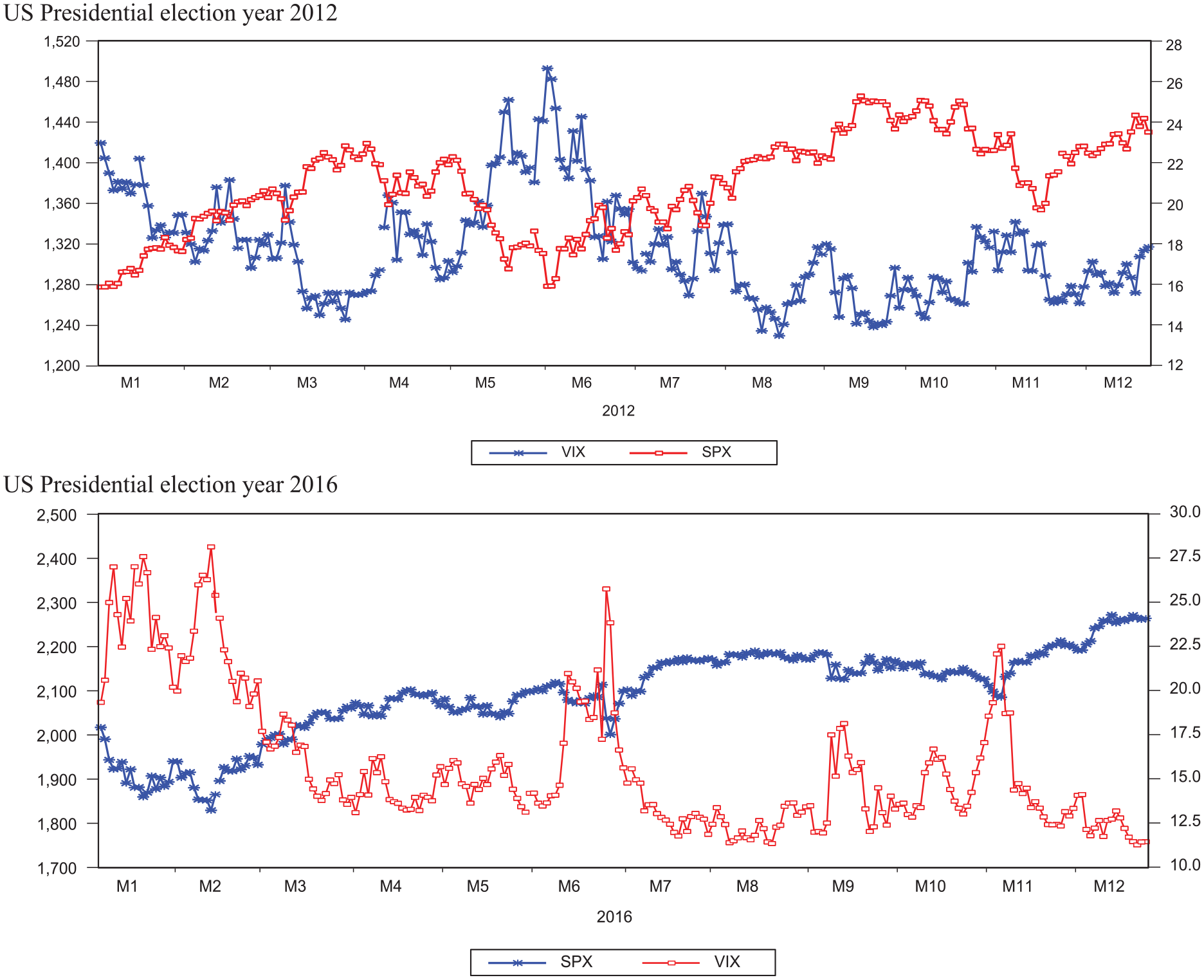
Time series plot of SPX and VIX under two presidential elections.

Figure 2.

SPX and VIX during October-December 2016.

Stylized X Pattern in the SPX Market

Figures 3 and 4 are the plots of the average change in the VIX and SPX returns based on election period and PEDs. More specifically, this entire graph speaks about the observation of move in VIX and returns on SPX on Election-Day, Pre-election-period, and Post-election-period. In addition, what happened to the market following the pre-scheduled PEDs between nominations of presidential candidates? Figure 3 shows that during the presidential election years 2012 and 2016, there was 2X pattern in the equity market. The market has performed identically following both the election years. But, when PEDs are under consideration, it is not correct. Generally speaking, the PED takes place during September and October before 10 to 12 trading days from the electoral voting day (second week of November, Tuesday). The election year 2012 reports 4X pattern, while 2016 shows 6X pattern. Hence, it is apparent from Figure 4 that the investors’ perception during the incumbent election year remains quite normal, while on the counterpart of the election year 2016, market has remained quite abnormal. The significant fall in the implied volatility (VIX) level (Post-election-period) is the calm before the storm, wait and watch. Hence, market efficiency within short-run does not hold good for the market. Investors try to eat abnormal profit during the election years.

Figure 3.

Average changes in the VIX and SPX returns.

Figure 4.

Average changes in the VIX and SPX returns during presidential elections debate.

Empirical Model Building

The present work analyzes the behavior of the investor sentiment measured by the CBOE volatility index, popularly known as the VIX, derived from the SPX index-based options. The daily closing prices of VIX, SPX, and 1-month T-Bill rate have been considered to account for the effects of two presidential elections (2012/2016). There are mainly three causes of the presidential ESM: first, change in the economic policy and the political stakes in presidential position; second, PECs and investment and consumption behavior; and third, the election creates political and social uncertainty. The political and social uncertainty has a potential impact on all asset class, and more specifically, it has pronounced effects in the equity market.

Let $V I X_{t}$ be the daily closing of implied volatility index, $S P X_{t}$ is the stock index, and $T B 1 M_{t}$ is the 1-month T-bill rate of the U.S. treasury market. The contemporaneous log-transformed returns are calculated as

R S P X_{t} = \ln {\frac{S P X_{t}}{S P X_{t - 1}}},

(1)

R T B 1 M_{t} = \ln {\frac{T B 1 M_{t}}{T B 1 M_{t - 1}}},

(2)

and the change in the implied volatility index is measured as

Δ V I X_{t} = V I X_{t} - V I X_{t - 1} .

(3)

The U.S. Presidential Elections and Investor Sentiment

The empirical model has been structured in the form of dummy variables to analyze the behavior of the future stock market volatility. The regression model presented below is the extension of Fleming, Ostdiek, and Whaley (1995), and the model also incorporates the 1-month T-bill rate to control for the risk-free rate.

\begin{array}{l} Δ V I X_{t} = δ_{0} + δ_{1}^{O c t} D_{t}^{O c t} + δ_{2}^{P r e_e l e c t i o n - 5 d a y} D_{t}^{P r e_e l e c t i o n - 5 d a y} \\ + δ_{3}^{E l e c t i o n_d a y} D_{t}^{E l e c t i o n_d a y} \\ + δ_{4}^{P o s t_e l e c t i o n + 5 d a y} D_{t}^{P o s t_e l e c t i o n + 5 d a y} \\ + δ_{5}^{P o s t_e l e c t i o n + 27 d a y} D_{t}^{P o s t_e l e c t i o n + 27 d a y} \\ + δ_{6}^{R S P X} {RSPX}_{t} + δ_{7}^{R T B 1 M} RTB 1 M_{t} \\ + δ_{8}^{Δ V I X_{t - 1}} Δ V I X_{t - 1} + ε_{t} . \end{array}

(4)

Variable description and hypotheses of the model:

$δ_{0}$	Intercept: the empirical model encompasses the intercept coefficient; it captures the market behavior during the presidential election year disregarding the election event window days. There are 59 event window days out of 244 (Year 2012) and 247 (Year 2016) trading days. Hence, apart from election movements, if any, events (e.g., economic, social, natural, international) occurred during the election year then, the intercept term should appear positive and statistically significant. In addition, if election year causes fear and concern about the market, then the intercept coefficient should appear positive for both the election years.
$D_{t}$	Dummy variable, assumes either 0 or 1
$D_{t}^{O c t}$	October is the pre-election month of the respective election years. The slope will subsume the market sentiment in terms of investors’ perception about the presidential candidate and their future election strategy. If there is high degree of ambiguity about the winner for president-elect, then, the slope should appear statistically significant.
$D_{t}$ variants	This dummy variable measures the effects of presidential election around election window i.e., i = −5, –4 . . . 0 . . . +1 . . . +5 or –10 and +10 day: $D_{t}^{P r e_e l e c t i o n - 5 d a y}$ Pre-election period (e.g., –5 to –1): VIX is the expected stock market volatility (e.g., Shaikh, 2017; 2019). It is irrespective of what contained in the political election polls and agenda that the unknown election results cause rise in the VIX level. The election uncertainty results into continuous increase in the implied volatility; the reason is the higher the nervousness results in buying more options to protect the market holding. More specifically, higher pressure on the put options increases the VIX level abnormally. Consequently, the slope coefficient on the pre-election period should appear positive and statistically significant. $D_{t}^{E l e c t i o n_d a y}$ Election day (0): Election day is the final electoral voting day for the presidential candidate, and that creates more ambiguity in the market. Therefore, on the day of election, the VIX should reach its peak level gauged as the highest fear and greed of the market participants. For this reason, the election days’ slope should appear positive and significant. $D_{t}^{P o s t_e l e c t i o n + 5 d a y}$ Post-election-period (+1 to +5): Post-election period is the resolving of the political beliefs and uncertainty. By counting on the electoral votes, the presidential candidate is to be declared as the winner. As the market uncertainty resolved, the slope coefficient for post-election window should appear negative and statistically significant. This is the trading period wherein the VIX adjusts itself and reverts back to the normal range.
$D_{t}^{P o s t_e l e c t i o n + 27 d a y}$	This dummy measures the stock market behavior in post-election period
$R S P X_{t}$	Long-transformed contemporaneous returns on SPX equity index
$R T B 1 M_{t}$	Returns on 1-month treasury bill rate
$Δ V I X_{t - 1}$	Change in the implied volatility index (VIX) one period lag
$ε_{t}$	Classical white noise term

PEDs and Stock Market Volatility

Forsythe et al. (1992) have presented the anatomy of an experiment of the PSM followed by PEDs. To examine the market price of the stock on the day t, Forsythe et al. (1992) have expressed the following model:

M_{t} = E_{t} {M_{t} | φ_{t - 1}} + γ [P_{t} - E_{t} {P_{t} | φ_{t - 1}}] D_{t} + ε'_{t},

(5)

where $M_{t}$ is the market price on day t; $E_{t}$ is the expectation operator, conditions upon information available before to time t ( $φ_{t - 1}$ ); $P_{t}$ is the outcome of the opinion poll declared on day t; $D_{t}$ is the dummy variable, assumes 0 or 1 depending on new poll declared on day t; $ε'_{t}$ is the classical white noise process.

The rationale of this model is that polls communicate the valuable market-wide information (new information/unanticipated) that influence the market prices. To implement the effects of PEDs on the variation of expected stock market volatility, the regression model expressed as follows:

\begin{array}{l} Δ V I X_{t} = γ_{0} + γ_{1}^{P E D_{1} - 5 d a y} D_{t}^{P E D_{1} - 5 d a y} + γ_{2}^{P E D_{1}} D_{t}^{P E D_{1}} \\ + γ_{3}^{P E D_{1} + 5 d a y} D_{t}^{P E D_{1} + 5 d a y} + γ_{4}^{P E D_{2} - 5 d a y} D_{t}^{P E D_{2} - 5 d a y} \\ + γ_{5}^{P E D_{2}} D_{t}^{P E D_{2}} + γ_{6}^{P E D_{2} + 5 d a y} D_{t}^{P E D_{2} + 5 d a y} \\ + γ_{7}^{P E D_{3} - 5 d a y} D_{t}^{P E D_{3} - 5 d a y} + γ_{8}^{P E D_{3}} D_{t}^{P E D_{3}} \\ + γ_{9}^{P E D_{3} + 5 d a y} D_{t}^{P E D_{3} + 5 d a y} + δ_{10}^{R S P X} R S P X_{t} \\ + δ_{11}^{R T B 1 M} R T B 1 M_{t} + δ_{12}^{Δ V I X_{t - 1}} Δ V I X_{t - 1} + ε'_{t}, \end{array}

(6)

where γ0 is the intercept; PED₁ = −5, –4…0…+ 1, +5; PED₂ = −5, –4…0…+ 1, +5; PED₃ = −5, –4…0…+ 1, +5; $D_{t}$ is the dummy variable that assumes 0 or 1 depending on PEDs on day t; and $ε'_{t}$ is the classical white noise term.

PEDs

The PEDs generally taking place between two leading presidential candidates nominated from the two parties. If the PED contains some meaningful information about the future strategy of the U.S. political economy, then the slope coefficient of the PED window should appear statistically significant. The negative (positive) significant slope signifies fear (greed) and anxiety among the market participant out of the recent debate winner.

Empirical Results and Discussion

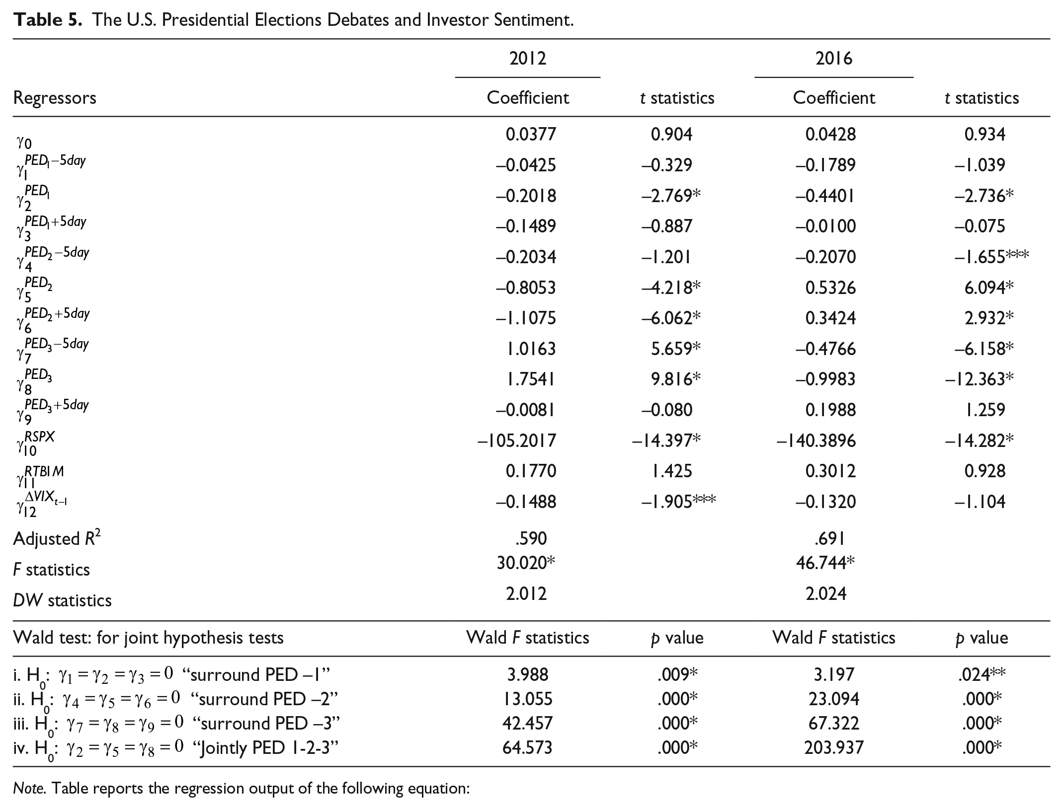
Tables 3 and 4 report the regression results on the behavior of future equity market volatility for the two U.S. presidential elections. Table 3 shows the regression output on election window of October, Pre-election period, Election Day, and Post-election period, and the election window consists of –5 and +5 days from the Election Day. Similarly, Table 4 shows the outcomes on variation in the equity market volatility of window –10 and +10 days. Table 5 presents the investors’ market participation around the PEDs. Besides, each table reports the Wald F test statistics, to test the joint hypothesis.

Table 3.

The U.S. Presidential Elections and Investor Sentiment With an Event Window of [–5, 0, +5, +27].

Regressors	2012	t statistics	2016	t statistics
Regressors	Coefficient	t statistics	Coefficient	t statistics
$δ_{0}$	0.0322	0.862	0.0211	0.451
$δ_{1}^{O c t}$	−0.0293	−0.360	0.0274	0.169
$δ_{2}^{P r e_e l e c t i o n - 5 d a y}$	0.1064	0.918	0.4092	1.911***
$δ_{3}^{E l e c t i o n_d a y}$	0.1668	1.657***	0.1007	0.429
$δ_{4}^{P o s t_e l e c t i o n + 5 d a y}$	−1.0972	−7.931*	−0.5217	−1.636***
$δ_{5}^{P o s t_e l e c t i o n + 27 d a y}$	0.1997	2.330*	0.1016	0.801
$δ_{6}^{R S P X}$	−108.1285	−18.925	−140.3930	−14.471*
$δ_{7}^{R T B 1 M}$	0.2140	1.771***	0.1852	0.598
$δ_{8}^{Δ V I X_{t - 1}}$	−0.2159	−2.871*	−0.1251	−1.044
Adjusted R2	.619		.706
$F statistics$	50.170*		71.228*
$D W statistics$	2.029		2.024
Wald test: for joint hypothesis tests	Wald F statistics	p value	Wald F statistics	p value
i. H₀: $δ_{1} = δ_{2} = 0$ “Pre-election period”	0.448	.640	1.834	.162
ii. H₀: $δ_{4} = δ_{5} = 0$ “Post-election period”	34.070*	.000	1.598	.204

Note. The table reports the regression output of the following equation:

$\begin{matrix} Δ V I X_{t} = δ_{0} + δ_{1}^{O c t} D_{t}^{O c t} + δ_{2}^{P r e_e l e c t i o n - 5 d a y} D_{t}^{P r e_e l e c t i o n - 5 d a y} \\ + δ_{3}^{E l e c t i o n_d a y} D_{t}^{E l e c t i o n_d a y} + δ_{4}^{P o s t_e l e c t i o n + 5 d a y} D_{t}^{P o s t_e l e c t i o n + 5 d a y} \\ + δ_{5}^{P o s t_e l e c t i o n + 27 d a y} D_{t}^{P o s t_e l e c t i o n + 27 d a y} + δ_{6}^{R S P X} R S P X_{t} \\ + δ_{7}^{R T B 1 M} R T B 1 M_{t} + δ_{8}^{Δ V I X_{t - 1}} Δ V I X_{t - 1} + ε_{t} . \end{matrix}$

The t statistic is based on Newey–West HAC consistent standard errors and covariance.

Significant at 1% level. ** Significant at 5% level. ***Significant at 10% level.

Table 4.

The U.S. Presidential Elections and Investor Sentiment With an Event Window of [–10, 0, +10, +27].

Regressors	2012	t statistics	2016	t statistics
Regressors	Coefficient	t statistics	Coefficient	t statistics
$δ_{0}$	0.0586	1.639***	0.0320	0.715
$δ_{1}^{O c t}$	−0.0207	−0.213	−0.1229	−0.779
$δ_{2}^{P r e_e l e c t i o n - 10 d a y}$	0.1920	1.371	−0.2044	−0.779
$δ_{3}^{E l e c t i o n_d a y}$	0.0164	0.134	0.0132	0.051
$δ_{4}^{P o s t_e l e c t i o n + 10 d a y}$	−0.1142	−0.846	−0.5942	−3.429*
$δ_{5}^{P o s t_e l e c t i o n + 27 d a y}$	−0.6092	−2.231**	−0.2258	−0.986
$δ_{6}^{R S P X}$	−105.9782	−16.403*	−140.0114	−14.463*
$δ_{7}^{R T B 1 M}$	0.1646	1.353	0.2193	0.703
$δ_{8}^{Δ V I X_{t - 1}}$	−0.1814	−2.516*	−0.1348	−1.130
Adjusted R2	.617		.697
$F statistics$	47.165*		71.407*
$D W statistics$	2.020		2.025
Wald test: for joint hypothesis tests	Wald F statistics	p value	Wald F statistics	p value
i. H₀: $δ_{1} = δ_{2} = 0$ “Pre-election period”	1.194	.305	0.389	.678
ii. H₀: $δ_{4} = δ_{5} = 0$ “Post-election period”	2.770	.065***	6.428	.002

Note. Table report the regression output of the following equation:

$\begin{matrix} Δ V I X_{t} = δ_{0} + δ_{1}^{O c t} D_{t}^{O c t} + δ_{2}^{P r e_e l e c t i o n - 10 d a y} D_{t}^{P r e_e l e c t i o n - 10 d a y} \\ + δ_{3}^{E l e c t i o n_d a y} D_{t}^{E l e c t i o n_d a y} + δ_{4}^{P o s t_e l e c t i o n + 5 d a y} D_{t}^{P o s t_e l e c t i o n + 5 d a y} \\ + δ_{5}^{P o s t_e l e c t i o n + 27 d a y} D_{t}^{P o s t_e l e c t i o n + 27 d a y} + δ_{6}^{R S P X} R S P X_{t} \\ + δ_{7}^{R T B 1 M} R T B 1 M_{t} + δ_{8}^{Δ V I X_{t - 1}} Δ V I X_{t - 1} + ε_{t} . \end{matrix}$

The t statistic is based on Newey–West HAC consistent standard errors and covariance.

Significant at 1% level. ** Significant at 5% level. ***Significant at 10% level.

Table 5.

The U.S. Presidential Elections Debates and Investor Sentiment.

Regressors	2012	t statistics	2016	t statistics
Regressors	Coefficient	t statistics	Coefficient	t statistics
$γ_{0}$	0.0377	0.904	0.0428	0.934
$γ_{1}^{P E D_{1} - 5 d a y}$	−0.0425	−0.329	−0.1789	−1.039
$γ_{2}^{P E D_{1}}$	−0.2018	−2.769*	−0.4401	−2.736*
$γ_{3}^{P E D_{1} + 5 d a y}$	−0.1489	−0.887	−0.0100	−0.075
$γ_{4}^{P E D_{2} - 5 d a y}$	−0.2034	−1.201	−0.2070	−1.655***
$γ_{5}^{P E D_{2}}$	−0.8053	−4.218*	0.5326	6.094*
$γ_{6}^{P E D_{2} + 5 d a y}$	−1.1075	−6.062*	0.3424	2.932*
$γ_{7}^{P E D_{3} - 5 d a y}$	1.0163	5.659*	−0.4766	−6.158*
$γ_{8}^{P E D_{3}}$	1.7541	9.816*	−0.9983	−12.363*
$γ_{9}^{P E D_{3} + 5 d a y}$	−0.0081	−0.080	0.1988	1.259
$γ_{10}^{R S P X}$	−105.2017	−14.397*	−140.3896	−14.282*
$γ_{11}^{R T B 1 M}$	0.1770	1.425	0.3012	0.928
$γ_{12}^{Δ V I X_{t - 1}}$	−0.1488	−1.905***	−0.1320	−1.104
Adjusted R2	.590		.691
$F statistics$	30.020*		46.744*
$D W statistics$	2.012		2.024
Wald test: for joint hypothesis tests	Wald F statistics	p value	Wald F statistics	p value
i. H₀: $γ_{1} = γ_{2} = γ_{3} = 0$ “surround PED –1”	3.988	.009*	3.197	.024**
ii. H₀: $γ_{4} = γ_{5} = γ_{6} = 0$ “surround PED –2”	13.055	.000*	23.094	.000*
iii. H₀: $γ_{7} = γ_{8} = γ_{9} = 0$ “surround PED –3”	42.457	.000*	67.322	.000*
iv. H₀: $γ_{2} = γ_{5} = γ_{8} = 0$ “Jointly PED 1-2-3”	64.573	.000*	203.937	.000*

Note. Table reports the regression output of the following equation:

$\begin{matrix} Δ V I X_{t} = γ_{0} + γ_{1}^{P E D_{1} - 5 d a y} D_{t}^{P E D_{1} - 5 d a y} + γ_{2}^{P E D_{1}} D_{t}^{P E D_{1}} + γ_{3}^{P E D_{1} + 5 d a y} D_{t}^{P E D_{1} + 5 d a y} \\ + γ_{4}^{P E D_{2} - 5 d a y} D_{t}^{P E D_{2} - 5 d a y} + γ_{5}^{P E D_{2}} D_{t}^{P E D_{2}} + γ_{6}^{P E D_{2} + 5 d a y} D_{t}^{P E D_{2} + 5 d a y} \\ + γ_{7}^{P E D_{3} - 5 d a y} D_{t}^{P E D_{3} - 5 d a y} + γ_{8}^{P E D_{3}} D_{t}^{P E D_{3}} + γ_{9}^{P E D_{3} + 5 d a y} D_{t}^{P E D_{3} + 5 d a y} \\ + δ_{10}^{R S P X} R S P X_{t} + δ_{11}^{R T B 1 M} R T B 1 M_{t} + δ_{12}^{Δ V I X_{t - 1}} Δ V I X_{t - 1} + ε'_{t} . \end{matrix}$

The t statistic is based on Newey–West HAC consistent standard errors and covariance.

Significant at 1% level. ** Significant at 5% level. ***Significant at 10% level.

Now, starting with the regression results shown in Table 3, the intercept coefficient appears to be positive for both the presidential election years, but not statistically significant (except to the election year 2012, Table 4). It can be understood that no major non-political events occurred that can affect the investors’ sentiment. The positive intercept also speaks that the market has remained in turbulent mode during the ESM. At this point, one can say that CBOE VIX is the barometer of the investors’ concerns and continue to be more volatile on ESM. The outcome for the election window (–10 days; +10 days) also shows similar results.

October is the month with the full amount of ambiguity of the U.S. presidential election leading to the poll day. The content of the election agenda occurs on large volumes with the flow of enormous market rumor. The slope of the month October of the election year 2012 appears to be negative while for the election year 2016, it is positive. Coefficients of October month are different from zero but not statistically significant. This evidences that when there is an incumbent party candidate in the election, history shows that the incumbent party always win the elections, the reason investor feels more precise about the election outcome. Unlike the election year 2012 and October month, the slope of October 2016 is estimated to be positive, albeit not statistically significant. The positive slope speaks when a presidential candidate is the new faces, for example, the election year 2016, the Republican candidate Donald Trump and Democrat Hillary Clinton. The unknown face and their political agendas make the investor more fearful during the election period. The slopes of October month in both the table appear to be statistically not significant also implies just not the timing of reflecting election news.

The Pre-election period (–5 days) is the primary strategic buy and hold period in the U.S. securities market. The market rally of bulls and bears and their aggressive participation yield the VIX at its highest level. It seems apparent from the Table 3 that the respective slopes of Pre-election period (–5 days) appears 0.1064 (Year 2012) and 0.4092 (Year 2016), and the slope of the year 2016 is calculated statistically significant at 10% level. The positive slope uncovers the fact that investor worries were higher before the Election Day. One can see that investors’ fear was 4 times more in the election year 2016 on the counterpart of 2012.

The Election Day’s slope of 2012 appears 0.1668, and for 2016, it was 0.1007. The coefficients are positive and significant at the 10% level (the election year 2012). This also implies that from the pre-election period to the poll day, VIX rises significantly, and it is happening due to unknown outcomes/polls of the election period.

The Post-election period (+5 days) is the period of the end of the election uncertainty. Once the electoral voting is done, counts are ready, and the winner is announced, the market is prepared to compound that information in fair price of stocks. The over-reaction to the unknown information remains higher than the known phenomenon. It is apparent from the regression estimates, respectively, –1.0972 (Year 2012) and –0.5217 (Year 2016), and statistically significant at 1% and 10% level. One can interpret that once the election polls are publicly available, then VIX goes its average level, for example, during the election year 2012, VIX level goes down by 1.09-point basis.

Moreover, the Post-election period (+27 days) also supports the previous outcomes. In the post-election period, the market becomes more confident, and VIX falls until it reaches its normal range. The summary statistics show that VIX ranges between 10% and 15% in the post-election period till the third week of December. The Wald F statistics have been reported in Tables 3 and 4 for the testing of a joint null hypothesis which seems to be statistically significant for the post-election period. The statistics signify that post-election period is the most stable period in which the investor does not trade aggressively.

Table 5 shows that the regression output on the PEDs took place during the last week of September and through October months. The PEDs are the most essential three political events that make the cognitive minds of the U.S. citizens about the presidential electoral votes. The PEDs are pre-announced and scheduled events taking place between the two presidential candidates (for more details, see Appendix B), each one from the leading political party. The PED forms the basis for the winning in the electoral votes and presents the point of view of each presidential candidate. The debate agenda and winner at the end of the debates decide the future of next U.S. president-elect. Table 5 provides some of the important insights about the change in the expected stock market volatility trailed by the respective PEDs. The minutes of the PEDs provide strategic guidelines to the market participants about the future movement in the economy as a whole. Hence, as the points raised in the PEDs, investors take their market positioning accordingly.

Looking at the PEDs of the election year 2012, the slope of the three respective contests appears to be –0.2018, –0.8053, and +1.7541 and statistically significant at 1% level. The significant estimate on PED indicates that the investor does regard the minutes of the PEDs in their portfolio selection. The first two presidential debates resulted into considerable fall in the level of VIX on the market opening, the third one has created the major upset among the market participants, and VIX was up by 1.75-point basis (i.e., 17%). Unlike the regime of the election year 2012, the slopes of three debates (Year 2016) appear, respectively, –0.4401, +0.5326, and –0.9983 and statistically significant at 1% level. It is apparent from the results that the market remains less volatile, and the level of VIX was falling at 0.44/0.99-point basis followed by each debate except to the second one. The plausible explanation for this phenomenon is that Hillary was leading Trump in all three PED debates. The Democrat candidate was a new face in U.S. politics with zero political experience. The conventional wisdom of the election 2016 was that Hillary would defeat Trump based on the observed polls of PED. Hence, the overreaction of the investor was marginal, and the market has adjusted for the Democrat lead over Republican. The Wald F statistics at the end of Table 5 shows the joint hypothesis test of the impact of PED on the ESM. It has been seen that for all PEDs, F statistics appear statistically significant. It also implies that investor jointly regard the PEDs in their portfolio planning.

Robustness Check

To further validate the results presented in “Empirical Results and Discussion” section, a robustness check has been performed using the Equation 4. An interaction dummy variable has been introduced in Equation 4 in terms of economic policy uncertainty (EPU). Baker, Bloom, and Davis (2016) propose an index of policy uncertainty that tracks the economic and political changes for the U.S. economy. Figure 5 depicts the relationship between VIX and EPU around the presidential election. It is seen that political uncertainty and investors’ sentiment is positively associated around the election period. The presidential election year 2012 exhibits frequent spikes in the VIX level following the political uncertainty. In the case of presidential election year 2016, investors’ sentiment index remains a more stable subject of political uncertainty. Hence, to model this relation, Equation 4 is further modified as

\begin{array}{l} Δ V I X_{t} = δ_{0} + δ_{j}^{O c t} \ln E P U D_{t}^{O c t} + \sum_{i = - 5}^{+ 5} δ_{j} \ln E P U D_{i t} \\ + \sum_{k = - 6}^{+ 27} δ_{j} \ln E P U D_{k t} + δ_{j}^{R S P X} R S P X_{t} \\ + δ_{j}^{R T B I M} R T B 1 M_{t} + δ_{j} Δ V I X_{t - 1} + ε_{t}, \end{array}

(6)

where EPU³ is the Economic Policy Uncertainty Index calculated by Baker et al. (2016). The term $\ln E P U D_{t}^{O c t}$ is the interaction dummy that measures the effects of political uncertainty on investors’ sentiment in the month of October and likewise specified for other variables.

Figure 5.

The relationship between political uncertainty (EPU) and investor sentiment (VIX).

Table 6 shows the robustness check of the outcome presented in the previous section. The regression results are reported separately for the election years 2012 and 2016 with event window of ±5, 0, ±10, 0, +22, and +27. It is apparent that the outcomes are in line with the previous results and literature evidence. One of the important observations is that the intercept coefficient appears to be positive for both the election years but not statistically significant. Based on a priori hypothesis, volatility should rise in the pre-election period (i.e., October) and it is valid for the election year 2016.

Table 6.

Economic Policy Uncertainty and Investor Sentiment Around Presidential Election 2012 and 2016.

Panel A: Presidential election year 2012
	Intercept	October	–5	0	+5		RSPX	RTB1M	$Δ V I X_{t - 1}$	F statistics
Coefficient	0.054	−0.009	0.018	0.027	–0.201 *		−107.782*	0.190	−0.205*	49.09*
t-stat	1.37	−0.26	0.32	0.01	−4.73		−19.32	1.40	−2.96
	Intercept	October	–5	0	+5	+27	RSPX	RTB1M	$Δ V I X_{t - 1}$	F statistics
Coefficient	0.029	−0.004	0.022	0.035	–0.198 *	0.038	−108.209*	0.218	−0.217*	44.32*
t-stat	0.74	−0.13	0.38	0.01	−4.75	1.36	−19.28	1.57	−3.16
	Intercept	October	–10	0	+10	+22	RSPX	RTB1M	$Δ V I X_{t - 1}$	F statistics
Coefficient	0.023	−0.001	0.001	0.026	–0.140 *	0.064**	−106.832*	0.213	−0.210*	43.85*
t-stat	0.57	−0.03	0.03	0.03	−4.33	2.10	−19.86	1.51	−3.09
Panel B: Presidential election year 2016
	Intercept	October	–5	0	+5		RSPX	RTB1M	$Δ V I X_{t - 1}$	F statistics
Coefficient	0.033	0.004	0.093 ***	0.021	–0.100 **		−140.459*	0.148	−0.124*	70.08*
t-stat	0.67	0.06	1.69	0.05	−1.97		−35.70	0.24	−4.37
	Intercept	October	–5	0	+5	+27	RSPX	RTB1M	$Δ V I X_{t - 1}$	F statistics
Coefficient	0.015	0.008	0.098 ***	0.023	–0.096 ***	0.034	−140.824*	0.130	−0.127*	62.45*
t-stat	0.28	0.14	1.72	0.06	−1.91	0.98	−34.82	0.21	−4.41
	Intercept	October	–10	0	+10	+22	RSPX	RTB1M	$Δ V I X_{t - 1}$	F statistics
Coefficient	0.010	−0.022	0.117 **	0.009	–0.067	0.049	−140.655*	0.128	−0.139*	63.27*
t-stat	0.20	−0.34	2.11	0.03	−1.44	1.44	−35.01	0.21	−4.92

Note. Table reports the regression output of the following equation

$\begin{matrix} Δ V I X_{t} = δ_{0} + δ_{j}^{O c t} \ln E P U D_{t}^{O c t} + \sum_{i = - 5}^{+ 5} δ_{j} \ln E P U D_{i t} + \sum_{k = - 6}^{+ 27} δ_{j} \ln E P U D_{k t} \\ + δ_{j}^{R S P X} R S P X_{t} + δ_{j}^{R T B 1 M} R T B 1 M_{t} + δ_{j} Δ V I X_{t - 1} + ε_{t} . \end{matrix}$

The t statistic is based on Newey–West HAC consistent standard errors and covariance. Bold numbers signify that estimates appear as per a priori hypothesis.

Significant at 1% level. ** Significant at 5% level. ***Significant at 10% level.

Moreover, before the poll day, VIX level should increase significantly (e.g., Nippani & Medlin, 2002; Shaikh, 2017) and it is correct for both the election years. The election ambiguity and investors’ belief about the next president-elect causes a significant rise in the stock market volatility. This phenomenon is found to be straightforward with the positive coefficient calculated for the pre-election window and poll day. Once the uncertainty gets resolved, VIX level should fall rapidly, and it reaches to the normal level. It is also relevant as looking at the coefficients of +5/+10/+22/+27 days appears to be negative and statistically significant (e.g., Allvine & O’Neill, 1980).

Conclusion

The present work aims to explain the effects of the U.S. presidential elections on the ESM in the form of investor sentiment index. The VIX is the implied volatility index based on the options written on the SPX index. It is one of the essential real-time measures of investor’s fear and greed. Hence, the study considered two presidential elections year 2012 and 2016 to examine its impact on the VIX level. The different aspect of the study is that this is the first attempt that models the future stock market volatility during the presidential election years.

The dummy variable technique has been employed to account for the effects of presidential elections on the stock mark volatility. The significant findings of the study are (a) the market was more turbulent before 1 week of the Election Day; (b) in the post-election period, VIX remained at a most normal level; and (c) the PED has shown significant impact on the strategic ESM performance.

The non-parametric test reveals the fact that both election years and ESM remained independent of each other in terms of performance. Furthermore, the work refutes the hypothesis of the PEC that effects on the stock market. The equity market passes the test of market efficiency in the long-run, but at the same time, ESM is not random during the presidential election period. Plausibly, the investors’ optimism with regard to presidential elections 2012/2016 remained higher under the Democrats beliefs, but on the counter part of the Republicans, it was somehow very low.

The policy/practical implication is of twofold: (a) the work explains the behavior of the investors’ fear and greed on the occasion of presidential elections and buy and hold strategy that impacts the VIX level and (b) the empirical findings confirm the market efficiency of SPX options market and VIX regarded as the barometer of investors’ concerns, and at the same time, it encourages the investor to trade in the volatility as an asset class in terms of F&O written on VIX index.

Footnotes

Appendix

Appendix B

Presidential election debate.

Presidential debates 2012
					Candidates			Result
Sr. No.	Date	Day	Place		Democrat	Republican		Winner
1	October 3, 2012	Wednesday	University of Denver, Denver		Obama	Romney		Obama
2	October 16, 2012	Tuesday	Hofstra University, Hempstead		Obama	Romney		Obama
3	October 22, 2012	Monday	Lynn University, Boca Raton		Obama	Romney		Obama
	Timing: 9 p.m. and 10:30 p.m. EDT
Presidential debates 2016
					Candidates			Result
Sr. No.	Date	Day	Place		Democrat	Republican		Winner
1	September 26, 2016	Monday	Hofstra University, New York’s		Hillary	Trump		Hillary
2	October 9, 2016	Sunday	Washington University, St. Louis		Hillary	Trump		Hillary
3	October 19, 2016	Wednesday	University of Nevada, Las Vegas		Hillary	Trump		Hillary
	Timing: 9:00 p.m. and 10:30 p.m. EDT
2012PE debate_1_3rd October 2012					2016PE debate_1_26th September 2016
Estimation window: January 3, 2012, to December 21, 2012, N = 245					Estimation window: January 4, 2016, to December 23, 2016, N = 248
Event window		Start date	End date	Observations	Event window	Start date	End date	Observations
Pre_Debate_1		October 3, 2012	September 27, 2012	5	Pre_Debate_1	September 26, 2016	September 20, 2016	5
Debate_1		October 4, 2012	October 4, 2012	1	Debate_1	September 27, 2016	September 27, 2016	1
Post_Debate_1		October 5, 2012	October 11, 2012	5	Post_Debate_1	September 28, 2016	October 04, 2016	5
Total				11	Total			11
2012PE debate_2_16th October 2012					2016PE debate_2_9th October 2016
Estimation window: January 3, 2012, to December 21, 2012, N = 245					Estimation window: January 4, 2016, to December 23, 2016, N = 248
Event window		Start date	End date	Observations	Event window	Start date	End date	Observations
Pre_Debate_2		October 16, 2012	October 10, 2012	5	Pre_Debate_2	October 7, 2016	October 3, 2016	5
Debate_2		October 17, 2012	October 17, 2012	1	Debate_2	October 10, 2016	October 10, 2016	1
Post_Debate_2		October 18, 12	October 24, 2012	5	Post_Debate_2	October 11, 2016	October 17, 2016	5
Total				11	Total			11
2012PE debate_3_22nd October 2012					2016PE debate_3_19th October 2016
Estimation window: January 3, 2012, to December 21, 2012, N = 245					Estimation window: January 4, 2016, to December 23, 2016, N = 248
Event window		Start date	End date	Observations	Event window	Start date	End date	Observations
Pre_Debate_3		October 22, 2012	October 16, 2012	5	Pre_Debate_3	October 19, 2016	October 13, 2016	5
Debate_3		October 23, 2012	October 23, 2012	1	Debate_3	October 20, 2016	October 20, 2016	1
Post_Debate_3		October 24, 2012	November 1, 2012	5	Post_Debate_3	October 21, 2016	October 27, 2016	5
Total				11	Total			11

Declaration of Conflicting Interests

The author(s) declared no potential conflicts of interest with respect to the research, authorship, and/or publication of this article.

Funding

The author(s) received no financial support for the research, authorship, and/or publication of this article.

ORCID iD

Imlak Shaikh

Notes

Author Biography

Imlak Shaikh is an assistant professor of accounting and finance at Management Development Institute (MDI), Gurgaon. Previously, he served as an assistant professor at the Birla Institute of Technology and Science (BITS), Pilani. He has also taught at IIM Rohtak as an adjunct faculty in FPM program. He received his post-graduation degree in commerce from the Veer Narmad South Gujarat University, Surat, and his PhD from Indian Institute of Technology Bombay (IIT Bombay). He has been awarded with “PhD Theses Excellence Award” from IIT Bombay. He has recently published in North American Journal of Economics and Finance, Engineering Economics, Journal of Business Economics and Management, Economic Change and Restructuring, Journal of Economic Studies, and so on.

References

Allvine

F. C.

O’Neill

D. E.

(1980). Stock market returns and the presidential election cycle: Implications for market efficiency. Financial Analysts Journal, 36(5), 49-56.

Baker

S. R.

Bloom

Davis

S. J.

(2016). Measuring economic policy uncertainty. The Quarterly Journal of Economics, 131, 1593-1636.

Bowen

R. M.

Castanias

R. P.

Daley

L. A.

(1983). Intra-industry effects of the accident at Three Mile Island. Journal of Financial and Quantitative Analysis, 18, 87-113.

Brander

J. A.

(1989). Election polls, free trade, and the stock market: Evidence from the Canadian general election (NBER Working Paper No. 3073). Retrieved from https://www.nber.org/papers/w3073

Browning

E. S

. (2000). Most stocks decline amid election worries: Stocks favoring bush climb, but NASDAQ falls 184.09 points. The Wall Street Journal, Thursday, November 9, C1.

Brüggelambert

(2004). Information and efficiency in political stock markets: Using computerized markets to predict election results. Applied Economics, 36, 753-768.

Chien

W.-W.

Mayer

R. W.

Wang

(2014). Stock market, economic performance, and presidential elections. Journal of Business & Economics Research, 12, 159-170.

Döpke

Pierdzioch

(2006). Politics and the stock market: Evidence from Germany. European Journal of Political Economy, 22, 925-943.

Ejara

D. D.

Nag

Upadhyaya

K. P.

(2012). Opinion polls and the stock market: Evidence from the 2008 US presidential election. Applied Financial Economics, 22, 437-443.

10.

Fleming

Ostdiek

Whaley

R. E.

(1995). Predicting stock market volatility: A new measure. Journal of Futures Markets, 15, 265-302.

11.

Foerster

S. R.

Schmitz

J. J.

(1997). The transmission of US election cycles to international stock returns. Journal of International Business Studies, 28(1), 1-13.

12.

Forsythe

Frank

Krishnamurthy

Ross

T. W.

(1998). Markets as predictors of election outcomes: Campaign events and judgement bias in the 1993 UBC election stock market. Canadian Public Policy/Analyse de Politiques, 24, 329-351.

13.

Forsythe

Nelson

Neumann

G. R.

Wright

(1992). Anatomy of an experimental political stock market. The American Economic Review, 82, 1142-1161.

14.

Forsythe

Rietz

T. A.

Ross

T. W.

(1999). Wishes, expectations and actions: A survey on price formation in election stock markets. Journal of Economic Behavior & Organization, 39, 83-110.

15.

Füss

Bechtel

M. M.

(2008). Partisan politics and stock market performance: The effect of expected government partisanship on stock returns in the 2002 German federal election. Public Choice, 135, 131-150.

16.

Hansen

Schmidt

Strobel

(2004). Manipulation in political stock markets–preconditions and evidence. Applied Economics Letters, 11, 459-463.

17.

Henry

P. B.

(2000). Stock market liberalization, economic reform, and emerging market equity prices. The Journal of Finance, 55, 529-564.

18.

Herbst

A. F.

Slinkman

C. W.

(1984). Political-economic cycles in the US stock market. Financial Analysts Journal, 40(2), 38-44.

19.

Herron

M. C.

Lavin

Cram

Silver

(1999). Measurement of political effects in the United States economy: A study of the 1992 presidential election. Economics & Politics, 11, 51-81.

20.

Hill

Schneeweis

(1983). The effect of Three Mile Island on electric utility stock prices: A note. The Journal of Finance, 38, 1285-1292.

21.

Hobbs

G. R.

Riley

W. B.

(1984). Profiting from a presidential election. Financial Analysts Journal, 40(2), 46-52.

22.

Homaifar

Randolph

W. L.

Helms

B. P.

Haddad

(1988). American presidential elections and returns of defence industry stocks. Applied Economics, 20, 985-993.

23.

Hood

Nofsinger

J. R.

(2008). Corporate PACs and the stock market: The case of the 2004 presidential election. The Journal of Wealth Management, 11, 93-103.

24.

Huang

R. D.

(1985). Common stock returns and presidential elections. Financial Analysts Journal, 41(2), 58-61.

25.

Hung

L.-C.

(2013). U.S. presidential elections and the Taiwanese stock market. Issues & Studies, 49(1), 71-97.

26.

Jang

C.-L.

Chang

C.-P.

(2016). Vote buying and victory of election: The case of Taiwan. Prague Economic Papers, 25, 591-606.

27.

Jensen

N. M.

Schmith

(2005). Market responses to politics: The rise of Lula and the decline of the Brazilian stock market. Comparative Political Studies, 38, 1245-1270.

28.

Knight

(2006). Are policy platforms capitalized into equity prices? Evidence from the Bush/Gore 2000 presidential election. Journal of Public Economics, 90, 751-773.

29.

Born

J. A.

(2006). Presidential election uncertainty and common stock returns in the United States. Journal of Financial Research, 29, 609-622.

30.

Lin

C. Y.

P. H.

Shen

C. H.

Wang

Y. C.

(2016). Political connection, government policy, and investor trading: Evidence from an emerging market. International Review of Economics & Finance, 42, 153-166.

31.

MacRae

C. D.

(1977). A political model of the business cycle. Journal of Political Economy, 85, 239-263.

32.

Mattozzi

(2008). Can we insure against political uncertainty? Evidence from the U.S. stock market. Public Choice, 137, 43-55.

33.

Niederhoffer

Gibbs

Bullock

(1970). Presidential elections and the stock market. Financial Analysts Journal, 26, 111-113.

34.

Nippani

Arize

A. C.

(2005). US presidential election impact on Canadian and Mexican stock markets. Journal of Economics and Finance, 29, 271-279.

35.

Nippani

Liu

Schulman

C. T.

(2001). Are treasury securities free of default? Journal of Financial and Quantitative Analysis, 36, 251-266.

36.

Nippani

Medlin

W. B.

(2002). The 2000 presidential election and the stock market. Journal of Economics and Finance, 26, 162-169.

37.

Nordhaus

W. D.

(1975). The political business cycle. The Review of Economic Studies, 42, 169-190.

38.

Pantzalis

Stangeland

D. A.

Turtle

H. J.

(2000). Political elections and the resolution of uncertainty: The international evidence. Journal of Banking & Finance, 24, 1575-1604.

39.

Roberts

B. E.

(1990). Political institutions, policy expectations, and the 1980 election: A financial market perspective. American Journal of Political Science, 34, 289-310.

40.

Shaikh

(2017). The 2016 U.S. presidential election and the Stock, FX and VIX markets. The North American Journal of Economics and Finance, 42, 546-563. doi:10.1016/j.najef.2017.08.014

41.

Shaikh

(2019). On the relationship between economic policy uncertainty and the implied volatility index. Sustainability, 11(6), Article 1628.

42.

Stovall

R. H.

(1992). Forecasting stock market performance via the presidential cycle. Financial Analysts Journal, 48(3), 5-8.

43.

Sturm

R. R.

(2009). The “other” January effect and the presidential election cycle. Applied Financial Economics, 19, 1355-1363.

44.

Sturm

R. R.

(2013). Economic policy and the presidential election cycle in stock returns. Journal of Economics and Finance, 37, 200-215.

45.

2016 election: Market reactions. (2016, November 11). The Wall Street Journal. Retrieved from http://www.wsj.com/livecoverage/markets-real-time-stocks-bonds-currency-commodities-11-07

46.

Zivney

T. L.

Marcus

R. D.

(1989). The day the United States defaulted on treasury bills. The Financial Review, 24, 475-489.

47.

Zouaoui

Nouyrigat

Beer

(2011). How does investor sentiment affect stock market crises? Evidence from panel data. The Financial Review, 46, 723-747.

The U.S. Presidential Election 2012/2016 and Investors’ Sentiment: The Case of CBOE Market Volatility Index

Abstract

Keywords

Introduction

Review of Earlier Studies

Data Description and Sources

Summary Statistics and U.S. Presidential Elections

Graphical Examination

Stylized X Pattern in the SPX Market

Empirical Model Building

The U.S. Presidential Elections and Investor Sentiment

PEDs and Stock Market Volatility

PEDs

Empirical Results and Discussion

Robustness Check

Conclusion

Footnotes

Appendix

Declaration of Conflicting Interests

Funding

ORCID iD

Notes

Author Biography

References