Sage Journals: Discover world-class research

Abstract

Observation Oriented Modeling is a novel approach toward conceptualizing and analyzing data. Compared with traditional parametric statistics, Observation Oriented Modeling is more intuitive, relatively free of assumptions, and encourages researchers to stay close to their data. Rather than estimating abstract population parameters, the overarching goal of the analysis is to identify and explain distinct patterns within the observations. Selected data from a recent study by Craig et al. were analyzed using Observation Oriented Modeling; this analysis was contrasted with a traditional repeated measures ANOVA assessment. Various pitfalls in traditional parametric analyses were avoided when using Observation Oriented Modeling, including the presence of outliers and missing data. The differences between Observation Oriented Modeling and various parametric and nonparametric statistical methods were finally discussed.

Keywords

Observation Oriented Modeling Ordinal Pattern Analysis individual analysis repeated measures ANOVA honeybee

Repeated measures ANOVA is a popular statistical technique widely used by a variety of research scientists. In most applications, the goal of the researcher is to examine changes over time on a single variable. For instance, a clinical psychologist may examine the long-term effectiveness of a therapeutic intervention by acquiring scores from a depression inventory on three different occasions: (a) 1 hr prior to the intervention, (b) 1 month post intervention, and (c) 1 year post intervention. By using repeated measures ANOVA, the researcher can assess the equivalence of mean levels of depression across the three measurement occasions. Of course, repeated measures ANOVA can also be used to address a much wider and more complex array of questions, especially when additional variables are assessed over time or when grouping variables are also examined. Researchers understand, nonetheless, that even for a simple study design, conducting a repeated measures ANOVA can be tricky business. One must worry about outliers, missing data, and a variety of assumptions (e.g., continuity, normality, homogeneity, and particularly sphericity). A choice must also be made between the traditional univariate, multivariate, and mixed-model approaches toward the analysis (Misangyi, LePine, Algina, & Goeddeke, 2006), and with this choice come additional concerns regarding corrections for Type I error inflation and the potential loss of statistical power (see Maxwell & Delaney, 2004).¹

In this article, we introduce a simple alternative to repeated measures ANOVA that requires fewer assumptions, is immune to outliers, and allows researchers to focus on the observations in hand rather than on the estimation of abstract population parameters. Researchers can also focus on assessing the accuracy of predicted patterns within the data rather than on the computation and interpretation of means and variances. Consequently, the issues underlying the choice between the univariate, multivariate, and mixed-model approaches to repeated measures ANOVA are completely eschewed. This novel and parsimonious alternative is referred to as an Ordinal Pattern Analysis in the context of Observation Oriented Modeling (Grice, 2011, 2014). Below, we demonstrate its features using a published data set that presented numerous problems for repeated measures ANOVA but that in contrast was easily analyzed using an Ordinal Pattern Analysis.

Repeated Measures ANOVA

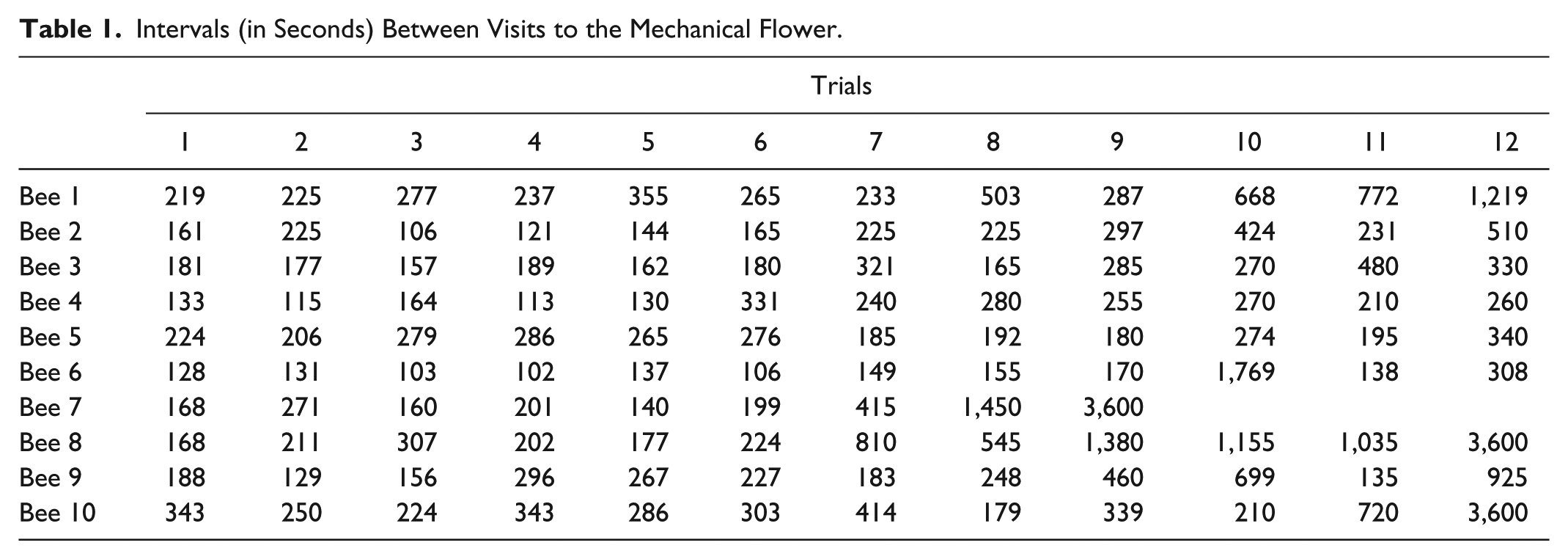
In a study on social reinforcement learning, Craig et al. (2012) captured and tagged honeybees to track their visits to an “artificial flower” in which the bees could consume a rewarding sucrose-rich solution. For the first six recorded visits, the bees were permitted to consume the sucrose solution and freely fly from the flower to return to the hive. Based on simple laws of learning, the bees were expected to return to the mechanical flower (an excellent source of food) at shorter and shorter intervals from the first visit to the sixth. The intervals between visits were referred to as Inter-Visit-Intervals, or IVIs. The bees were then “frustrated” for six consecutive visits by trapping them for several minutes in the mechanical flower after they had consumed the sucrose solution, thus delaying their return to the hive. For these trials, the bees were expected to return to the flower at longer and longer intervals as the “frustration” of being trapped in the flower affected their behavior.

IVI measurements, reported in seconds, for 10 bees across the 12 trials are presented in Table 1. The maximum interval for a bee to return to the mechanical flower was set at 60 min (3,600 s), and all subsequent trials were treated as missing data if the bee returned several hours later, failed to return at all, or was observed foraging at a nearby open feeder with a less attractive source of sucrose (note Bees 7, 8, and 10 in Table 1). The recorded IVIs are considered independent between bees but dependent across trials and are thus suitable for analysis using a repeated measures ANOVA. As can be seen in Table 1, however, several features of the data are alarming. First, the 3,600 values are problematic because, although they fulfill a useful data management function, they represent extreme cases that could unduly affect the means for any given trial. Second, a single missing value on any one of the 12 trials could result in that bee being omitted depending on the type of analysis chosen. Finally, extreme times other than the 3,600 values may unduly influence the mean for any particular trial and consequently affect the ANOVA results as well. Indeed, the means and standard errors plotted in Figure 1 show the impact of the extreme times (>1,000 s) for Trials 8 through 12.

Table 1.

Intervals (in Seconds) Between Visits to the Mechanical Flower.

	Trials
	1	2	3	4	5	6	7	8	9	10	11	12
Bee 1	219	225	277	237	355	265	233	503	287	668	772	1,219
Bee 2	161	225	106	121	144	165	225	225	297	424	231	510
Bee 3	181	177	157	189	162	180	321	165	285	270	480	330
Bee 4	133	115	164	113	130	331	240	280	255	270	210	260
Bee 5	224	206	279	286	265	276	185	192	180	274	195	340
Bee 6	128	131	103	102	137	106	149	155	170	1,769	138	308
Bee 7	168	271	160	201	140	199	415	1,450	3,600
Bee 8	168	211	307	202	177	224	810	545	1,380	1,155	1,035	3,600
Bee 9	188	129	156	296	267	227	183	248	460	699	135	925
Bee 10	343	250	224	343	286	303	414	179	339	210	720	3,600

Figure 1.

Inter-Visit-Interval means and standard errors for the 12 trials with and without extreme cases.

As might be expected, the results from the omnibus ANOVA with all of the extreme values included yielded a highly significant univariate omnibus F value, F(11, 88) = 4.61, p < .001, η² = .37. However, a number of questions raise concerns about this result. Because the data were analyzed in SPSS using the General Linear Model option (i.e., the traditional univariate approach to repeated measures ANOVA), all of the data for the seventh honeybee were excluded automatically from the analysis. Should the missing data be replaced with estimated IVI times? Replacing missing data routinely rests on the Missing at Random or more restrictive Missing Completely at Random assumptions (see Fox-Wasylyshyn & El-Masri, 2005, for a pithy review), which may not be the case for these data. However, no matter how the missing data are finally handled, the extreme 3,600 values and other outliers are still present. Perhaps these values should be deleted and replaced as well, or perhaps some type of transformation should be applied to the data.

Matters are made more difficult by the small number of honeybees relative to the number of trials. Even with a complete set of observations, the data could not be analyzed with the mixed-models approach (e.g., using the Mixed Model option in SPSS on restructured data; see Little, Milliken, Stroup, Wolfinger, & Schabenberger, 2006; Pinheiro & Bates, 2000, for discussions of mixed-model ANOVA), and the multivariate F value using the General Linear Model option in SPSS could not be computed due to insufficient degrees of freedom. The traditional univariate approach to repeated measures ANOVA was therefore the only option for testing the omnibus null hypothesis (as stated below), and this approach routinely requires an adjustment for violation of the sphericity assumption. When the Greenhouse–Geisser correction is applied, the degrees of freedom decrease to 1.46 and 11.68, yielding a p value of .042. The Huynh–Feldt correction reduces the degrees of freedom to 1.70 and 13.62, yielding a p value of .034. Finally, the lower-bound correction reduces the degrees of freedom to 1 and 8, yielding a non-significant p value of .064. It is widely recommended that researchers use one of these corrections to the univariate F value due to its sensitivity to violations of the sphericity assumption (Maxwell & Delaney, 2004). Which correction should be chosen here, and what of the other assumptions underlying the accuracy of the p value? Are additional transformations to the data or statistical adjustments necessary? With this question for these troublesome data, and without even arriving at more interesting specific mean comparisons, it should be clear that Frankenstein’s monster is potentially at hand . . . and he will be all too willing to lead his creator into misguided interpretations and conclusions.

Observation Oriented Modeling

What is needed for these types of “difficult” data is an Ordinal Pattern Analysis (OPA), which is simple, relatively free of assumptions, and yields results that are transparent and easily interpretable (Thorngate & Edmonds, 2013). Conducted within the wider context of Observation Oriented Modeling (Grice, 2011), this analysis also prompts an overall shift in perspective. Traditional statistics, such as the ANOVA example above, represent what Breiman (2001) refers to as the modeling approach to data. This approach regards data to be the result of stochastic processes, and analyses are centered on model fitting and parameter estimation. Binary decisions are also often made with regard to the fitted models (e.g., “the linear model was statistically significant”) and estimated parameters (“the null hypothesis, µ = 0, was rejected”).

In contrast, the observation oriented modeler regards data to be the result of a generative causal mechanism. In the ideal case, the researcher will in fact construct an iconic model describing the structures and processes underlying the data (e.g., Grice, 2015; Grice, Barrett, Schlimgen, & Abramson, 2012). The goal of the analysis is therefore to identify theoretically meaningful and robust patterns with the given observations (data), which is more akin to what Breiman (2001) referred to as algorithmic modeling. Because patterns are sought, the computation of means, variances, covariances, and so on, is unnecessary, nor is it necessary to use a particular statistical model (e.g., the General Linear Model). The entire null hypothesis significance testing paradigm, which underlies the binary decisions in traditional statistics, is also replaced by analyses that (a) involve careful visual examination of data using the “eye test” (or “interocular traumatic test,” Edwards, Lindman, & Savage, 1963) and (b) provide the tools necessary for determining which observations are consistent with the theoretically meaningful pattern. Determining the overall accuracy of the explanatory model is therefore tantamount, leading to an increase or decrease of confidence in the model.

To demonstrate the shift in perspective from data modeling and repeated measures ANOVA to Observation Oriented Modeling and OPA, we reanalyzed portions of Craig et al.’s (2012) original data. The complete design of Craig et al.’s study was quite complex, including 23 IVIs and 3 experimental and 1 control group of honeybees (total N = 50). For the purposes of demonstrating OPA and comparing it with ANOVA, we examined only the first 12 IVIs and only 2 groups of honeybees. This subset of the original data was sufficient to demonstrate the occurrence of learning in the honeybees (OPA results for the complete design can be found in Craig et al.), and it facilitated the presentation of various predicted patterns (via simpler graphs) as well as the exploration of novel analyses not reported by Craig et al. (viz., analyses involving predicted stability of IVIs).

Testing Patterns

As demonstrated in Craig et al.’s article, the shift in perspective from data modeling to Observation Oriented Modeling starts at the beginning, that is, with the hypotheses. With a repeated measures ANOVA, the goal is to estimate population parameters from the observed data, and in the framework of null hypothesis significance testing the null hypothesis is stated as follows:

H_{0} : μ_{1} = μ_{2} = μ_{3} = μ_{4} = μ_{5} = μ_{6} = μ_{7} = μ_{8} = μ_{9} = μ_{10} = μ_{11} = μ_{12}

In other words, all 12 population means are hypothesized to be equal. The omnibus alternative hypothesis is that 2 or more of these 12 population means are not equal. More specific alternative hypotheses could be advanced contrasting pairs or groups of population means.

Given these hypotheses, however, it is important to realize that Craig et al. (2012) had no interest in estimating population parameters. Indeed, it is not clear what honeybees would constitute the imaginary population. Would the population only include forager honeybees (Apis mellifera ligustica) of approximately 3 to 6 weeks of age from the two hives that were sampled in the study, or would the population include nurse bees, drones, and the queens of the two hives? Should the population instead equal the global population of Apis mellifera ligustica, or should it include all subspecies of Apis mellifera in the world? How far, exactly, should the sample be generalized? Unfortunately, there is simply no way to answer these questions in a non-arbitrary manner, which is not to suggest that populations are always defined arbitrarily or that estimating population parameters is never worthwhile. In political polling, games of chance, and research in which a random or representative sample can be drawn from a clearly specified population, for example, parameter estimation can prove fruitful; but none of these instances covers Craig et al.’s study, nor are they representative of the authors’ scientific goals.

Like the majority of behavioral researchers, Craig et al. (2012) were instead attempting to explain the behavior of honeybees. In other words, they were interested in making an abductive inference (Douven, 2011) to the causes underlying honeybee behavior rather than making a statistical inference to population parameters (Grice, 2015; Haig, 2005, 2014). Abductive inference

involves reasoning from claims about phenomena, understood as presumed effects, to their theoretical explanation in terms of underlying causal mechanisms. Upon positive judgments of the initial plausibility of these explanatory theories, attempts are made to elaborate on the nature of the causal mechanisms in question. (Haig, 2008, pp. 1019-1020)

Abduction is also consistent with the philosophical realism underlying Observation Oriented Modeling, which encourages scientists to develop integrated, causal models that explain the observations made in a given study (see Grice, 2011, 2014, 2015; Grice et al., 2012, for examples). Turning one’s focus to abduction rather than statistical inference leads to a number of startling and liberating realizations. First, because population parameters are not necessarily being estimated, issues such as inferential errors (Type I, II, or III; Harris, 1997), statistical power, and parameter bias can fall by the wayside. As will be made explicit below, the goal in Observation Oriented Modeling is to identify meaningful and improbable patterns of observations (i.e., behaviors) of individual honeybees. Second, aggregate statistics such as means, variances, and covariances can be avoided not only as population parameters, but avoided in the analyses altogether. Causes operate at the level of the individuals and serve as the necessary conditions for each bee’s behavior. Causes do not affect means or other aggregate statistics directly, and hence the traditional, Galtonian/Fisherian/Pearsonian ways of thinking about data are not required. The Observation Oriented Modeler is thus not restricted to the use of inferential statistical methods and traditional mean- and variance-based analyses, and is instead ready to approach the order of nature in novel ways.

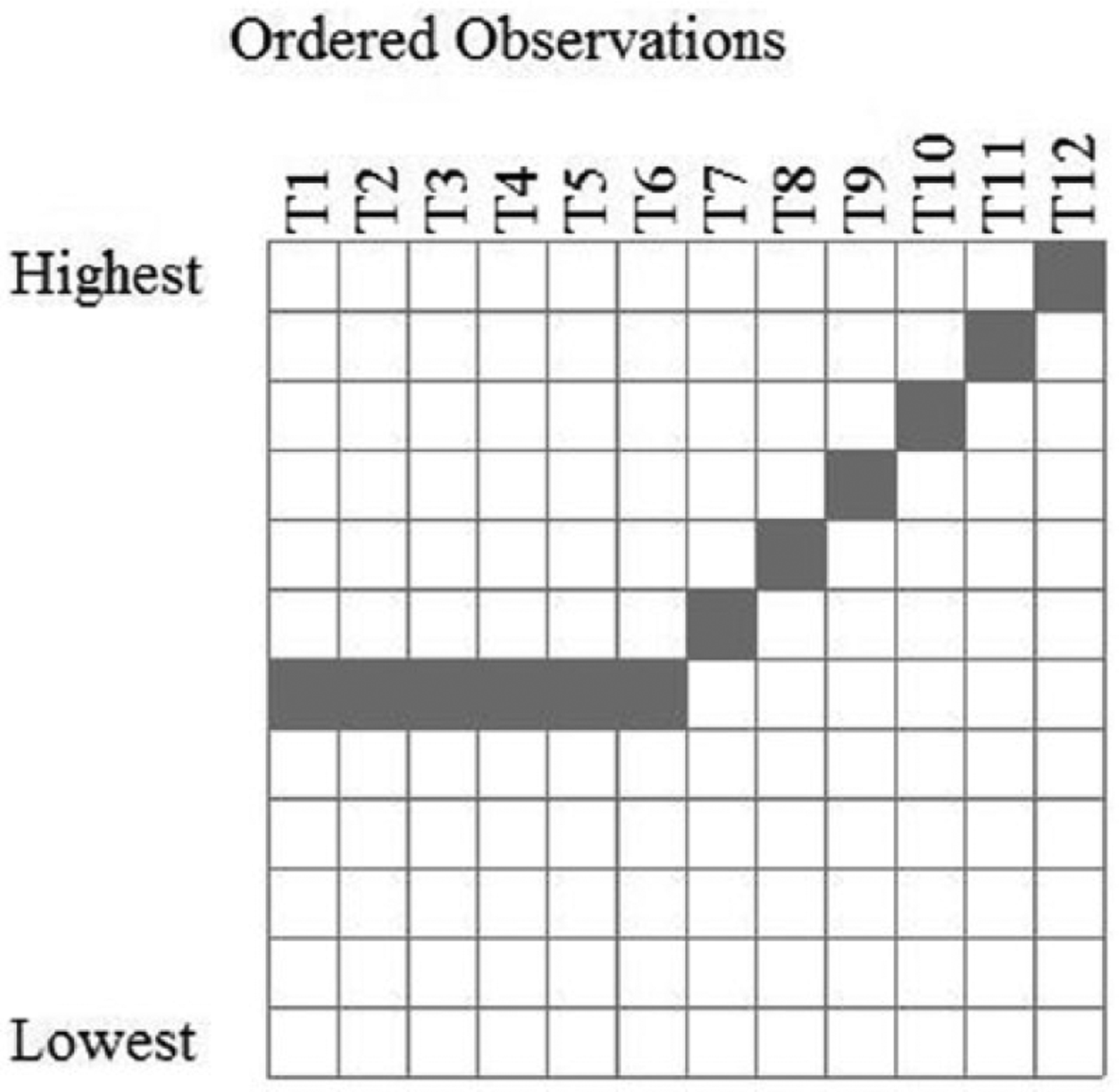
As mentioned above, in Observation Oriented Modeling, the focus is placed on patterns of observations. Craig et al. (2012) clearly expected a particular pattern in the recorded IVIs based on their understanding of the laws of learning. The pattern they expected and tested is ordinal, and it is a pattern that should match the observed values for every honeybee in their sample; hence, the proper level of analysis (see Trafimow, 2014) is the recorded IVI times for each bee. With this in mind, the expected pattern of ordinal relations can be defined in the OOM software as shown in Figure 2. As can be seen, the matrix in the figure is comprised of 12 rows, with the top and bottom rows labeled as “Highest” and “Lowest,” respectively. The columns are comprised of the 12 trials, and the shaded cells indicate the expected pattern of ordinal relations among the observed IVI times. As described above, each bee was expected to return to the mechanical flower faster and faster from Trials 1 through 6 (i.e., the IVIs were expected to decrease). After being “frustrated” by being trapped in the flower, each bee was then expected to take increasingly longer times to return to the flower (i.e., the IVIs were expected to increase). Moreover, the longest time for Trials 1 through 6 was expected to be shorter than the shortest time for Trials 7 through 12; in other words, every IVI for Trials 1 to 6 was expected to be shorter than every IVI for Trials 7 to 12.

Figure 2.

Expected ordinal pattern for IVI times for each honeybee across the 12 trials.

With the expected pattern determined based on the researchers’ understanding of the causes behind the data, the observations for each honeybee can be examined. Figure 3 shows the results for the sixth bee in Table 1. As can be seen, her recorded IVI times matched the ordinal pattern closely. In OOM, there are two ways to quantify the fit between the observations and the expected ordinal pattern. First, only adjacent trials (i.e., the columns in Figure 3) can be considered, namely, 1 versus 2, 3 versus 4, 5 versus 6, and so on. With 12 trials, there are 11 pairs of adjacent trials. If the ordinal relation for a bee’s observations matches the expected ordinal relation for any pair of adjacent trials, then the pair of observations is considered as “correctly classified.” Using this adjacent counting method, the honeybee in Figure 3 produced eight correctly classified pairs of observations. Converting this result to a percentage yields the Percent Correct Classification (PCC) index for this honeybee, which is the primary numerical value to be obtained from analyses in OOM. For this bee, the PCC index is 72.73% (8/11) and is fairly impressive.

Figure 3.

Expected (shaded cells) and observed (1s) ordinal relations for the sixth frustrated honeybee’s IVI times across the 12 trials.

Second, all possible pairs of observations can be considered, namely, 1 versus 2, 1 versus 3, . . . 1 versus 12, 2 versus 3, 2 versus 4, . . . 2 versus 12, and so on. With 12 trials, there are 66 (₁₂C₂ = 66) pairs of observations that can be classified as correctly matching the ordinal pattern. The number of correct classifications for the honeybee in Figure 3 using this more stringent criterion is 54, yielding a PCC index equal to 81.82%, an impressive result. This second approach for classifying pairs of observations is said to be more stringent because it takes into account the entire pattern rather than only adjacent pairs of observations. The hypothetical data in Figure 4, for instance, fit the expected pattern perfectly (PCC = 100%) when considering only adjacent observations, but only 36 of the 66 pairs of observations (PCC = 54.55%) are correctly classified if the entire pattern is considered. The decision to use either method would ideally be driven by a causal, integrated model (Grice, 2011), but as will be shown below, using both methods for computing the PCC values for the same data may be pragmatically beneficial.

Figure 4.

Hypothetical data for which the PCC index equals 100% when considering only adjacent observations, but equals only 54.55% when considering all pairs of observations.

Using the option to match the entire pattern, the results for each honeybee are summarized in Table 2. As can be seen, the number of correctly classified pairs of observations is tallied and converted to the PCC index. Obviously, the PCC index ranges from 0 to 100, and the expectation here is that each value will equal 100, indicating perfect accuracy for the ordinal pattern. Not a single honeybee matched the pattern perfectly, all but one yielded PCC indices of at least 60%, whereas four bees’ PCC indices were at least 80%, which is fairly impressive given the strict method of attempting to match the entire pattern.

Table 2.

Individual Classification Results for All 10 Bees.

	Observations	Missing cases	Classifiable pairs of observations	Correct classifications	PCC value	c-value
Bee 1	12	0	66	48	72.73	.02
Bee 2	12	0	66	53	80.30	<.01
Bee 3	12	0	66	50	75.76	.01
Bee 4	12	0	66	43	65.15	.10
Bee 5	12	0	66	26	39.39	.84
Bee 6	12	0	66	54	81.82	<.01
Bee 7	9	3	36	30	83.33	.01
Bee 8	12	0	66	53	80.30	<.01
Bee 9	12	0	66	41	62.12	.16
Bee 10	12	0	66	40	60.61	.16

Note. PCC = Percent Correct Classification.

A probability statistic, referred to as a c-value (or chance value), is also reported in Table 2 for each honeybee. It was computed by first randomizing the data within trials for each bee. Consider, for example, values for a single bee from three consecutive trials: 140, 200, and 100. A randomized version of these data could be 200, 100, and 140. The PCC index is next computed for the randomized data on the basis of the expected ordinal pattern, and the process is repeated for a set number of times (1,000 randomized trials for the current analysis). The PCC indices are recorded, and the number of times the actual observed PCC index is equaled or exceeded for each honeybee is tallied and converted to a proportion. A high c-value near one therefore indicates that randomized versions of the same data routinely yielded PCC values as high or higher than the actual PCC value. In other words, the observed PCC index was not unusual. A low c-value near zero, on the other hand, indicates that the observed PCC index was rather unusual because it was not readily equaled or exceeded by PCC indices from randomized versions of the actual data. The chance value is therefore a randomization test, and it is reported as a “c-value” rather than a “p value” to remind researchers that it is an assumption-free probability derived from repeated randomizations of the actual data (e.g., no assumptions of normality, homogeneity, and so on, are made; see Winch & Campbell, 1969, for an early discussion of randomization tests; see Edgington & Onghena, 2007; Manly, 1997, for more recent treatments).

Examination of the c-values in Table 2 reveals that the observed results were highly improbable for all but the fifth honeybee. The PCC index for this bee was only 39.39, and her results in Figure 5 show that, for some unknown reason, her IVIs were often shorter (indicating faster returns to the flower) after being trapped in the flower. No other information about this particular bee helped to explain her unexpected behavior, but it is clear OOM provides the tools necessary for focusing on the individual honeybees rather than on means or the estimation of abstract population parameters.

Figure 5.

Data for the fifth frustrated honeybee.

Table 2 also shows that missing data can be handled at the level of the individual bees. IVI times were not recorded for Trials 10 to 12 for the seventh bee. The number of possible pairs of observations was thus reduced from 66 to 36, and the PCC index was computed on the basis of the 36 possible correct classifications. The result was impressive (83.33%) for the seventh honeybee, and the c-value (.01) again indicated that the result was improbable. As another option for handling missing data, the PCC index can be computed on the basis of the original possible pairs of observations, 66 in this case. Using this option for the seventh honeybee, the PCC index drops to 45.45% (30/66) with a c-value equal to .61, thus indicating the impact of the missing data. In addition to the missing data, the extreme values in the data set (see Table 1) posed no problems for the analysis because it is based on ordinal relations much like other non-parametric statistical procedures (see Cliff, 1996). No adjustments were necessary to the data themselves nor to the analysis itself.

The results for all of the bees considered together can also be examined. These results are printed in the OOM software as follows:

Classification Results : All Observations

Ordinal Relations between Pairs of

Observations Classified According to the

Defined Pattern(s)

Classifiable Pairs of Observations : 630

Correct Classifications : 438

Percent Correct Classifications : 69.52

Classifiable Complete Cases : 9

Correctly Classified Complete Cases : 0

Percent Correct Classified Cases : 0.00

Randomization Results : All Observations

Observed Percent Correct Classifications : 69.52

Number of Randomized Trials : 1000

Minimum Random Percent Correct : 38.10

Maximum Random Percent Correct : 60.16

Values >= Observed Percent Correct : 0

Model c-value : less than ( 1 / 1000); that is, < 0.001

Observed Percent Correct Classified Cases : 0.00

Number of Randomized Trials : 1000

Minimum Random Percent Correct Cases : 0.00

Maximum Random Percent Correct Cases : 0.00

Values >= Observed Percent Correct Cases : 1000

Model c-value : 1.00

The Classifiable Pairs of Observations represents the total number of pairs of observations that can be classified correctly in the analysis. The value here, 630, equals the sum of the Classifiable Pairs of Observations reported in Table 2, and it can be seen that the missing pairs of observations for the seventh bee have been excluded. Of the 630 non-missing pairs across all of the bees and all of the trials, 438 were consistent with the ordinal pattern in Figure 2 and reported as Correct Classifications, yielding a fairly impressive PCC index of almost 70% (PCC = 69.52). The results from a randomization test show that not a single PCC index from 1,000 randomized versions of the data equaled or exceeded 69.52 (min = 38.10, max = 60.16) the observed PCC index. The c-value is thus less than 1 in 1,000, or c-value < .001. With additional randomizations of the data, a PCC value of at least 69.52 could still be observed. Finally, the Correctly Classified Complete Cases in the output above shows that not one of the nine honeybees (or cases) with non-missing data fit the entire pattern perfectly; PCC = 0, with a c-value necessarily equal to 1.

The results for all 10 honeybees are arguably good with the overall PCC index equal to 69.52% and most of the individual bee PCC indices greater than 60%. Still, as with an omnibus ANOVA, a question to ask of the current analysis is whether or not most of the correct classifications are a result of comparing the trials prior to and after trapping the bees in the artificial flower. It may be the case, for instance, that the observations (recorded IVI times) do not fit the pattern in Figure 2 very well for Trials 1 to 6 nor for Trials 7 to 12, but that the first 6 IVIs are generally lower than the 6 IVIs after the bees were trapped in the flower. To address this possibility, the IVIs were analyzed for only the first six trials and using the expected decreasing ordinal pattern for only those trials. The overall PCC index was low (PCC = 42.67%, c-value = .90), and the PCC indices for 8 of the 10 bees were less than 50%. The remaining two PCC indices were 53.33% and 60.00%. Next, the last six trials were analyzed, again using the expected increasing ordinal pattern for those trials. The overall PCC index was higher (PCC = 73.19%, c-value < .001), and the PCC indices for all but one of the bees (the fourth bee) were greater than 65%, with four values equal to or greater than 80%. These results, considered with those for the complete pattern above, indicate that the IVIs did not generally decrease from the first to sixth trials, but the times were greater for Trials 7 through 12 while also increasing in a monotonic rate for all but one bee.

Last, much like pairwise comparisons following an omnibus repeated measures ANOVA, all pairs of IVI values across all 12 trials can be examined in a manner consistent with the expected ordinal relations shown in Figure 2. Table 3 reports the results from these analyses, which clearly show the ordinal predictions for the first 6 trials do not fit the observations very well. Most PCC indices for these pairwise comparisons were 50% or lower, again indicating that the IVI times did not decrease in a monotonic fashion. When comparing IVI values from Trials 1 to 6 with Trials 7 to 12 in pairwise fashion, the PCC indices were all quite high. Most percentages were 80% or higher, and five values were 100%. Consistent with the conclusions above, trapping the honeybees in the mechanical flower led to higher IVI values. Last, pairwise comparisons for the last six trials showed the IVI values to be increasing in a somewhat monotonic fashion, with most PCC indices equal to or greater than 66%.

Table 3.

PCC Indices and c-Values for Predicted Ordinal Pairwise Comparisons of IVI Times.

PCC	1	2	3	4	5	6	7	8	9	10	11
1
2	50.00
3	60.00	50.00
4	30.00	50.00	40.00
5	50.00	40.00	40.00	60.00
6	30.00	70.00	30.00	50.00	30.00
7	80.00	80.00	80.00	70.00	70.00	60.00
8	70.00	60.00	80.00	60.00	70.00	60.00	60.00
9	80.00	90.00	90.00	80.00	80.00	80.00	70.00	70.00
10	88.89	88.89	77.78	77.78	88.89	66.67	88.89	88.89	77.78
11	77.78	88.89	77.78	77.78	77.78	66.67	66.67	66.67	44.44	22.22
12	100	100	100	100	100	88.89	100	88.89	100	66.67	88.89
c-values	1	2	3	4	5	6	7	8	9	10	11
1
2	0.62
3	0.35	0.62
4	0.91	0.61	0.79
5	0.61	0.84	0.83	0.38
6	0.95	0.15	0.95	0.64	0.94
7	0.05	0.01	0.05	0.18	0.18	0.38
8	0.17	0.26	0.04	0.35	0.19	0.36	0.25
9	0.07	0.01	0.01	0.05	0.05	0.05	0.17	0.17
10	0.02	0.01	0.1	0.08	0.02	0.26	0.01	0.02	0.1
11	0.09	0.01	0.09	0.08	0.07	0.28	0.25	0.26	0.74	0.98
12	0.001	0.001	0.003	0.001	0.002	0.02	0.001	0.02	0.001	0.27	0.02

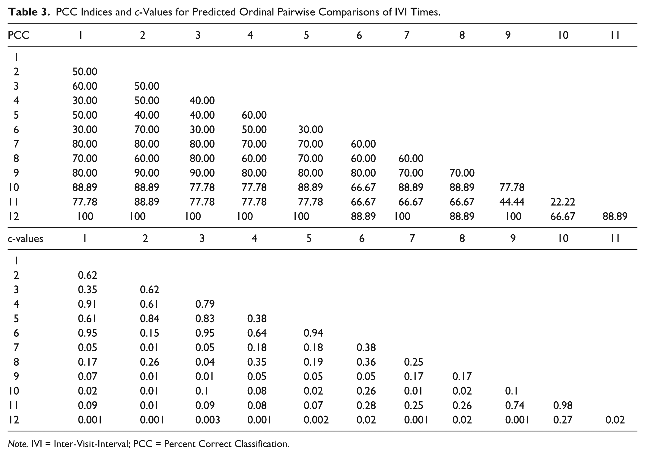
Note. IVI = Inter-Visit-Interval; PCC = Percent Correct Classification.

Testing Equivalence

Craig et al. (2012) also examined a group of 10 honeybees (see Table 4) who were allowed to fly freely from the mechanical flower for all 12 trials. These bees were not expected to demonstrate learned “frustration” like the other bees. Craig et al.’s analysis of the observed IVI times for these bees indeed revealed remarkably poor fit to the ordinal pattern in Figure 5. For the sake of demonstration in this article, let us now suppose that the IVI times were not expected to change substantially from trial to trial. Indeed, if the times for each bee were expected to be exactly equal across all trials, then the predicted ordinal pattern would be defined as shown in Figure 6. It would of course be unrealistic to expect perfect equality for each bee in this study. Numerous other causes are at work influencing the bees’ behavior, including activity in the hive, fatigue, weather conditions, and temperature. Consequently, the pattern in Figure 6 is tested in the OOM software using an imprecision setting. Ideally, such a setting would be based on previous observations, studies, or precise theory, but here it will be set in a somewhat arbitrary fashion. Specifically, it is reasonable to expect each honeybee to return to the flower within 2 min of each trial given the proximity of the hive to the mechanical flower and the sorts of delays any given bee might encounter when flying, entering the hive, and unloading her social crop. The question then is, given a range of ±120 s, will the IVI times match the ordinal pattern in Figure 6? In other words, will each bee return to the mechanical flower within 2 min each time, from the first trial to the last?

Table 4.

Intervals (in Seconds) Between Visits to the Mechanical Flower.

	Trials
	1	2	3	4	5	6	7	8	9	10	11	12
Bee 1	154	127	507	342	161	217	93	97	117	107	126	109
Bee 2	166	161	265	120	118	128	141	150	147	182	150	152
Bee 3	152	133	225	228	169	184	259	143	282	404	202	234
Bee 4	111	125	209	93	159	96	209	130	136	201	164	176
Bee 5	151	152	95	280	212	102	278	281	107	111	91	246
Bee 6	225	192	214	126	249	202	120	199	222	133	229	230
Bee 7	129	179	168	183	203	254	203	195	238	184	184	194
Bee 8	129	128	287	136	149	163	143	129	202	119	135	147
Bee 9	858	235	22	253	333	300	335	300	230	545	210	335
Bee 10	741	972	407	1,377	387	1,242	504	686	801	729	950	589

Figure 6.

Predicted pattern of equal IVI times for each honeybee across the 12 trials.

The results from the OOM software for the individual honeybees are shown in Table 5 and indicate an impressive degree of conformity between the observations and the expected pattern with the ±120 s imprecision setting. The PCC index was equal to 100% for the fourth bee, and the indices for four other bees were more than 80%. Only the IVI times for the 10th bee revealed very poor agreement with the expected ordinal pattern. As can be seen in Table 4, her IVIs ranged from 387 to 1,377 s and did not reveal any clear pattern across the 12 trials. The magnitudes of her times were generally high when compared with the other 9 bees, but no explanation could be found for why she was slow and for the variable in her IVI times.

Table 5.

Individual Classification Results for Pattern of Equality.

	Observations	Classifiable pairs of observations	Correct classifications	PCC value	c-value
Bee 1	12	66	44	66.67	0.41
Bee 2	12	66	62	93.94	0.03
Bee 3	12	66	51	77.27	0.22
Bee 4	12	66	66	100.00	0.01
Bee 5	12	66	39	59.09	0.62
Bee 6	12	66	64	96.97	0.02
Bee 7	12	66	65	98.48	0.01
Bee 8	12	66	56	84.85	0.09
Bee 9	12	66	39	59.09	0.62
Bee 10	12	66	12	18.18	1.00

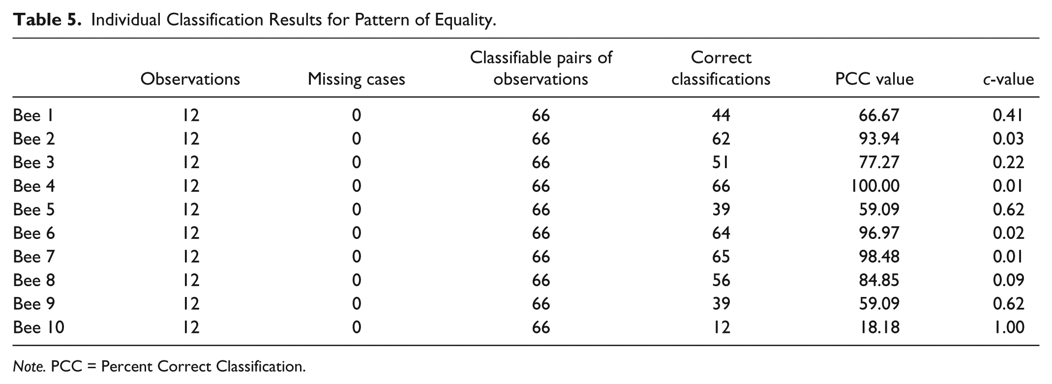
Note. PCC = Percent Correct Classification.

When equivalent patterns such as the one shown in Figure 6 are examined, the c-values will always equal 1 if all pairs of observations are being compared and the data are randomized as described above. Imagine, for example, IVI times for 3 trials equal to 100, 125, and 115, and a randomized order of these values as 125, 115, and 100. The absolute differences between all possible pairs of the original observations will equal the differences for the randomized values, namely, 25, 15, and 10. No matter how many times the IVI observations are randomized, this equality will always result, yielding the same PCC index in every case and a c-value of 1. Consequently, a randomization method that randomizes across (not just within) the bees is necessary for these types of patterns. For these data, we randomized both within all 12 IVI trials and across all 10 honeybees to compute the c-values reported in Table 5. As can be seen, 6 of the 10 values were .20 or lower, indicating improbable PCC indices. Not surprisingly, the c-value for the 10th bee was high (1.0 for 1,000 randomized trials).

Finally, as with the original analyses above, OOM permits the researcher to focus on the individual bees under investigation as well as allows the researcher to examine the overall data, even with this type of pattern. The results for all 10 bees yielded an impressive PCC index of 75.45% when comparing all possible pairs of IVI times for the 12 trials. The accompanying c-value was also impressively low (<.001).

Comparative ordinal patterns can also be constructed and evaluated to support the equality pattern shown in Figure 6. For instance, a monotonically decreasing pattern from Trials 1 through 12, with the imprecision setting of ±120 s, yielded an overall PCC index equal to 13.18%, c-value = .35. Tellingly, not one randomized PCC value equaled or exceeded 75.45%, the result for the equivalence pattern in Figure 6. Moreover, the individual PCC indices were below 50% for each of the 10 bees, and 9 of the 10 values were below 30%. Similarly dismal results were obtained when examining a monotonically increasing pattern across the 12 trials (overall PCC = 11.36, c-value = .69). In summary, the IVI times for the free-flying (non-frustrated) honeybees conformed well to the ordinal pattern of equivalence in Figure 6 with the imprecision setting of ±120 s. Data for only 1 of the 10 bees clearly did not fit this pattern. All other individual PCC indices were 59% or higher, and five were at least 80% (see Table 5).

Comparing Groups

Data from repeated measures and between-participants experimental designs can be combined in one analysis commonly referred to as a split-plot ANOVA, although it is sometimes referred to as a mixed-design ANOVA (Maxwell & Delaney, 2004). The data in Tables 1 and 4 are from 2 different groups of honeybees, and when compared across the 12 trials, constitute a 2 × (12) split-plot, factorial design. The primary reason for creating a factorial design is to assess the interaction between the two variables. The main effects may also be of interest but are often considered secondary and must be interpreted in the context of the interaction. With ANOVA, a statistically significant interaction is followed by either a simple-main-effects breakdown or the construction of interaction contrasts to understand the exact nature of the effect. Simple-main-effect breakdowns are more prevalent in the literature, but they conflate the variance of the interaction with the variance from one of the main effects. Interaction contrasts, by comparison, are “pure” follow-up tests of the interaction and have consequently been endorsed by a number of prominent methodologists (Harris, 1994; Rosnow & Rosenthal, 1995). An interaction contrast essentially describes how the pattern of means for one of the independent variables differs across levels of the other independent variable. For example, for Craig et al.’s data, a positive linear trend in the IVI means across all 12 trials for the frustrated honeybees could be contrasted with a negative linear trend for the free-flying bees.

Analysis of split-plot designs in Observation Oriented Modeling and the OOM software is akin to testing an interaction contrast, except the analysis is not based on means and variances and does not involve the estimation of population parameters. As with the OOM analyses above, ordinal patterns are constructed and then evaluated against the observations themselves. Beginning with free-flying bees, recall the ordinal pattern in Figure 6 (with the ±120 s imprecision setting) was a fairly accurate representation of the IVI times: overall PCC = 75.45, c-value < .001. All but 1 of the 10 bees conformed to this pattern at least reasonably well. In the spirit of an interaction contrast, how well does this pattern fit the IVI times for the frustrated honeybees? The results indicated overall unimpressive accuracy (PCC = 52.54, c-value = .03), although the IVI times for the fifth frustrated honeybee (see Table 1) were remarkably stable within ±120 s (PCC = 92.42). IVI times from three other frustrated honeybees were also somewhat consistent with the pattern (PCCs = 61%-68%), but a small majority nonetheless were not consistent with the pattern (i.e., six frustrated bees with PCCs < 50%).

Drawing on the original analyses above for the frustrated bees, an alternative competing pattern is shown in Figure 7. As can be seen, the IVI times are expected to be relatively stable across the first six trials and then increase monotonically from Trials 7 through 12. Again, the imprecision setting can be used, and for this analysis, any increases in IVI times for the last 6 trials must therefore exceed 120 s to be considered as correct classifications. The overall results for the frustrated honeybees using this ordinal pattern were good, but not highly impressive (PCC = 63.02%, c-value < .001). The fourth, fifth, and sixth bees’ IVI times (see Table 1) did not fit the pattern very well (PCCs < 52%), whereas the remaining majority of individual IVI times yielded PCC indices that exceeded 60%.

Figure 7.

Predicted pattern of IVI times for each honeybee across the 12 trials.

Evaluating the IVI times for the free-flying honeybees on the basis of the predicted ordinal pattern in Figure 7 yielded a very low overall PCC index (24.55%, c-value = .78). The PCC indices for the 10 free-flying bees were all below 50%, with seven values below 30%. Comparing the two distributions of overall PCC indices from the randomization test of each analysis furthermore revealed that an absolute difference of at least 38.47% (63.02 − 24.55) did not occur once in 1,000 trials (max = 20.35). The c-value for the difference between the overall PCC indices for the frustrated and free-flying bees was thus less than .001.

In summary, the free-flying honeybees returned to the mechanical flower at a fairly steady rate (±120 s), as measured by their IVI times. Only one bee showed a high degree of variability in her IVI times, and no discernable pattern was noticeable in her observations. A slight majority of the frustrated honeybees did not conform to the equivalent ordinal pattern (see Figure 6) that captured the free-flying bees so well. The ordinal pattern in Figure 7 offered a better explanation of the observations for these bees as it demarcated when they were frustrated by being trapped in the flower after the sixth trial. The IVI times for a slight majority of the bees (6 of the 10 bees) conformed to this predicted pattern with an imprecision setting of ±120 s. By successfully contrasting the patterns of observations for the free-flying and frustrated honeybees, results from these analyses support Craig et al.’s theoretical goal of demonstrating the occurrence of learning.

Discussion

Comparing parametric ANOVA with OPA in the novel analysis of data from Craig et al.’s (2012) study revealed a number of distinct advantages for the latter approach. First and foremost was the relative ease of conducting the analyses. When performing a repeated measures ANOVA, a seemingly ambiguous choice must be made between the traditional univariate, multivariate, and mixed-model approaches toward analyzing the data. Interestingly, this choice was made academic for Craig et al.’s data because of insufficient degrees of freedom for computing the omnibus test statistics for the multivariate and mixed-model approaches. Despite its many limitations, the traditional univariate approach therefore had to be used and one of the adjustments for Type I error inflation (e.g., Greenhouse–Geiger) chosen and applied. The necessity of these adjustments in turn points to the sensitivity of the univariate F test to violations of assumptions, particularly the sphericity assumption. Moreover, the analysis ignored the missing data problem, the 3,600 values, and the numerous influential IVI times. Addressing these issues would require difficult and sometimes assumption-laden decisions to make the data more suitable for analysis, including analyses involving more specific hypotheses about the 12 means. The conclusion is that conducting a repeated measures ANOVA for even a straightforward experimental design such as Craig et al.’s can be a complicated statistical affair.

By comparison, the analyses in the OOM software were simple and unambiguous. The expected pattern of ordinal relations was defined for the group of honeybees being analyzed, and the conformity between the actual observations and pattern for each bee was summarized with the PCC index. A simple, assumption-free and distribution-free randomization test was used in an entirely secondary role to help evaluate each individual and group-level PCC index. The homogeneity of treatment-difference population variances (sphericity) assumption and other assumptions underlying repeated measures ANOVA were therefore avoided entirely. The PCC index itself is transparent and readily interpretable by scientists and lay people alike. The η² value for the first group of honeybees analyzed above (the “frustrated” group) was equal to .37, indicating 37% overlap between the trials (the independent variable) and the IVI times (the dependent variable). It is difficult to interpret exactly what this measure of effect size means without the aid of arbitrary conventions (e.g., Cohen’s, 1988; Ferguson, 2009), and it is impossible to apply this effect size to any given bee in the sample. The individual PCC indices, however, are clearly interpretable, ranging from 0% to 100%, and indicate how well a bee’s IVI times matched the predicted ordinal pattern. All that is needed is the predicted pattern and the options chosen to compute the PCC index (i.e., the adjacent or complete options, and the imprecision value); otherwise, it requires no special knowledge or conventions to be interpreted and conveyed to a lay person. Its meaning can be made even more obvious when presented with a graphic like Figure 3. Recent scholarship (Kazdin, 1999; Thompson, 2002) points to the importance of transparent indices of practical and clinical “significance” (or relevance), and the PCC index and visual features of OPA are well suited for conveying such information.

The capability of examining all of the honeybees’ IVI times as a group as well as examining each individual bee is another advantage of the Observation Oriented Modeling approach. This is particularly important for Craig et al. because their goal, like most scientists, was abduction rather than statistical inference. The predicted ordinal patterns were based on simple laws of learning derived from other species (e.g., decreasing run times for a rat in a maze across trials; Greenough, Madden, & Fleischmann, 1972). The laws are general in the sense that they should apply to any given honeybee, not because they are descriptions of population parameters. In other words, the laws are causal, and the causes inhere in the honeybees themselves, not in abstract population parameters. Another way to understand the point being made here is that in repeated measures ANOVA, the goal is to describe patterns of sample and inferred population means, and these patterns may not match a single honeybee’s pattern of IVI times. For Craig et al., the proper level of analysis (Trafimow, 2014) is the individual bee, lest in describing the average, they end up describing “nobody in particular” (Vautier, Lacot, & Veldhuis, 2014, p. 51).

Seeking an inference to best explanation (i.e., abduction), it is noteworthy an alternative predicted pattern for the frustrated group of bees was constructed. Specifically, the original predicted decline in IVI times for the first six trials was replaced by an unchanging ordinal pattern (±120 s), and then the frustrated and free-flying bees were compared with regard to the new pattern. The unchanging part of the pattern can be explained sufficiently when considering the study more closely. There is a limit to how fast honeybees can fly, and each bee must make her way through the active hive to unload her crop. Such factors may essentially cancel out any decreases in IVI times across the first six trials due to learning. In addition, prior to data collection, Craig et al. were obliged to shape multiple participants’ responding in the artificial flower. After participants learned to reliably respond, two participants were concurrently run and the remaining trained participants were allowed to revisit the artificial flower before the next two participants’ data collection commenced. In short, the amount of pre-training was not controlled between participants, nor was the number of reinforcers and returns to the artificial flower. Consequently, the bees may have had sufficient pre-training such that decreases in IVI times across the first six trials would be minimal, at best, a conjecture supported by the relatively stable IVI times for the free-flying bees. Additional experimental work would be required to fully support these explanations, but the point is clear: In Observation Oriented Modeling, traditional statistical concerns are minimized, whereas efforts to seek theoretical explanations are magnified.

Another statistical issue that was eschewed in the OOM software was the influence of outliers in Craig et al.’s data. The analyses reported above were based on ordinal relations between trials and could therefore be regarded as a type of nonparametric statistical analysis, without the necessity of estimating population parameters. When considering the bees individually or all together in the context of the predicted ordinal pattern, it is difficult to relate the ordinal analysis to any specific nonparametric technique. Friedman’s Test and Kendall’s W (Siegel, 1956), for instance, are nonparametric alternatives to repeated measures ANOVA, but they are based on analysis of ranks and do not provide the means for assessing predicted ordinal patterns such as those posited by Craig et al. Nonetheless, it is well known that nonparametric statistics are generally less restricted by assumptions and are relatively immune to outliers (Cliff, 1996; Siegel, 1956). The OPA feature in the OOM software shares these advantages as it provides a flexible method for testing complex ordinal patterns that can be defined and assessed visually (e.g., see Figure 3) and numerically (viz., the PCC indices) for each case or for all the cases combined. Thorngate and Carroll (1986) long ago described and called for such ordinal methods they hoped would return the emphasis of theory and analysis to individuals and away from aggregate statistics and the estimation of abstract population parameters. Thorngate and Edmonds (2013) provide more recent examples of how their own OPA technique can be used to model crime rates and ratings of happiness.

It should be mentioned in closing that OPA can be used to test predicted parametric patterns, such as linear or quadratic functions. Describing how this is done is beyond the scope of this article, but it entails testing ordinal patterns for difference scores (assuming equal intervals between observations) using the imprecision option if necessary. Specific parametric predictions can moreover be tested. For instance, suppose Craig et al. possessed sufficient experimental control and theoretical power to predict the exact IVI values for each honeybee. The predicted values could be compared with the actual values across all 12 trials either exactly or within a set range (e.g., ±10 s) to obtain the PCC indices and c-values for each bee and for all of the observations combined. The techniques demonstrated in this article are thus flexible and capable of modeling different types of data and a wide array of patterns. These techniques are also easy to use and yield results that are transparent and readily interpretable.

Footnotes

Declaration of Conflicting Interests

The author(s) declared no potential conflicts of interest with respect to the research, authorship, and/or publication of this article.

Funding

The author(s) received no financial support for the research and/or authorship of this article.

Notes

Author Biographies

James W. Grice is professor of psychology at Oklahoma State University where he has taught courses in statistics, personality, psychological testing, and personalism for the past fourteen years. He is author of Idiogrid, a program for personality assessment, currently in use in over 30 countries around the world. He is also author of Observation Oriented Modeling: Analysis of Cause in the Behavioral Sciences (Academic Press, 2011) and the accompanying OOM software.

David Philip Arthur Craig developed an appreciation of comparative psychology prior to enrolling at the University of Florida where he cultivated a high degree of skepticism of population parameters and aggregate analyses. While attending Oklahoma State University, Dr. Craig began utilizing individual analyses to assess behavioral data from a variety of species for both practical and theoretical reasons.

Charles I. Abramson is Regents professor of psychology and Lawrence Boger professor of international studies. His area of research is the comparative analysis of behavior.

References

Breiman

(2001). Statistical modeling: The two cultures. Statistical Science, 16, 199-231.

Cliff

(1996). Ordinal methods for behavioral data analysis. Mahwah, NJ: Lawrence Erlbaum.

Cohen

(1988). Statistical power analysis for the behavioral sciences (2nd ed.). New York, NY: Routledge.

Craig

D. P. A.

Grice

J. W.

Varnon

C. A.

Gibson

Sokolowski

M. B. C.

Abramson

C. I.

(2012). Social reinforcement delays in free-flying honey bees (Apis mellifera L.). PLoS ONE, 7, e46729.

Douven

(2011), Abduction. In Zalta

E. N.

(Ed.), The Stanford encyclopedia of philosophy. Retrieved from http://plato.stanford.edu/archives/spr2011/entries/abduction/

Edgington

Onghena

(2007). Randomization tests (4th ed.). London, England: Chapman & Hall.

Edwards

Lindman

Savage

(1963). Bayesian statistical inference for psychological research. Psychological Review, 70, 193-242.

Ferguson

C. J.

(2009). An effect size primer: A guide for clinicians and researchers. Professional Psychology: Research and Practice, 40, 532-538. doi:10.1037/a0015808

Fox-Wasylyshyn

S. M.

El-Masri

M. M.

(2005). Handling missing data in self-report measures. Research in Nursing & Health, 28, 488-495.

10.

Greenough

W. T.

Madden

T. C.

Fleischmann

T. B.

(1972). Effects of isolation, daily handling, and enriched rearing on maze learning. Psychonomic Science, 27, 279-280.

11.

Grice

J. W.

(2011). Observation Oriented Modeling: Analysis of cause in the behavioral sciences. New York, NY: Academic Press.

12.

Grice

J. W.

(2014). Observation Oriented Modeling: Preparing students for the research in the 21st century. Innovative Teaching, 3, Article 3. doi:10.2466/05.08.IT.3.3

13.

Grice

J. W.

(2015). From means and variances to persons and patterns. Frontiers in Psychology, 6, 1007. doi: 10.3389/fpsyg.2015.01007

14.

Grice

J. W.

Barrett

P. T.

Schlimgen

L. A.

Abramson

C. I.

(2012). Toward a brighter future for psychology as an observation oriented science. Behavioral Sciences, 2, 1-22.

15.

Haig

B. D.

(2005). An abductive theory of scientific method. Psychological Methods, 10, 371-388.

16.

Haig

B. D.

(2008). Précis of “An abductive theory of scientific method.” Journal of Clinical Psychology, 64, 1019-1022. doi:10.1002/jclp.20506

17.

Haig

B. D.

(2014). Investigating the psychological world. Cambridge, MA: MIT press.

18.

Harris

R. J.

(1994). Analysis of variance primer. Itasca, IL: Peacock.

19.

Harris

R. J.

(1997). Significance tests have their place. Psychological Science, 8, 8-11.

20.

Kazdin

(1999). The meanings and measurement of clinical significance. Journal of Consulting and Clinical Consulting, 67, 332-339.

21.

Little

R. C.

Milliken

G. A.

Stroup

W. W.

Wolfinger

R. D.

Schabenberger

(2006). SAS for mixed models. Cary, NC: SAS Institute.

22.

Manly

(1997). Randomization, Bootstrap, and Monte Carlo methods in biology (2nd ed.). London, England: Chapman & Hall.

23.

Maxwell

S. E.

Delaney

H. D.

(2004). Designing experiments and analyzing data: A model comparison approach (2nd ed.). Belmont, CA: Wadsworth.

24.

Misangyi

LePine

Algina

Goeddeke

(2006). The adequacy of repeated-measures regression for multilevel research. Organizational Research Methods, 9, 5-28. doi:10.1177/1094428105283190

25.

Pinheiro

J. C.

Bates

D. M.

(2000). Mixed-effects models in S and S-Plus. New York, NY: Springer.

26.

Rosnow

Rosenthal

(1995). “Some things you learn aren’t so”: Cohen’s paradox, Asch’s paradigm, and the interpretation of interaction. Psychological Science, 6, 3-9.

27.

Siegel

(1956). Nonparametric statistics for the behavioral sciences. New York, NY: McGraw-Hill.

28.

Thompson

(2002). “Statistical,” “practical,” and “clinical”: How many kinds of significance do counselors need to consider? Journal of Counseling & Development, 80, 64-80.

29.

Thorngate

Carroll

(1986). Ordinal Pattern Analysis: A strategy for assessing hypotheses about individuals. In Valsiner

(Ed.), The individual subject and scientific psychology (pp. 201-232). New York, NY: Plenum Press.

30.

Thorngate

Edmonds

(2013). Measuring simulation-observation fit: An introduction to Ordinal Pattern Analysis. Journal of Artificial Societies and Social Simulation, 16(2), 4.

31.

Trafimow

(2014). The mean as a multilevel issue. Frontiers in Psychology: Quantitative Psychology and Measurement, 4, 451. doi:10.3389/fpsyg.2014.00180

32.

Vautier

Lacot

É.

Veldhuis

(2014). Puzzle-solving in psychology: The neo-Galtonian vs. nomothetic research focuses. New Ideas in Psychology, 33, 46-53.

33.

Winch

Campbell

(1969). Proof? No. Evidence? Yes. The significance of tests of significance. The American Sociologist, 4, 140-143.

A Simple and Transparent Alternative to Repeated Measures ANOVA

Abstract

Keywords

Repeated Measures ANOVA

Observation Oriented Modeling

Testing Patterns

Testing Equivalence

Comparing Groups

Discussion

Footnotes

Declaration of Conflicting Interests

Funding

Notes

Author Biographies

References