
Abstract
This study estimates a reduced-form regression model for mortality rates due to alcoholic liver diseases, with alcohol prices and income as explanatory variables. Panel data cover the years 2000-2010 for 21 member countries of the European Union. In the reduced form, prices affect mortality rates indirectly through the demand for alcohol, while income has potential direct and indirect effects. Country and time fixed effects are used to control for other factors that influence alcohol consumption and mortality. Special attention is paid to outliers in the data, and final results are based on the MS-estimator for robust regressions. Regression results for alcohol prices and income are sensitive to adjustments for stationary data and down-weighting of outliers and other influential data points. Final results indicate that alcohol prices do not affect mortality rates due to chronic liver diseases. Empirical results in the study do not lend support to broad price-based approaches to alcohol policy.
Introduction
Excessive use of alcohol is related to a variety of acute and chronic negative health outcomes, including injuries and deaths from traffic accidents, cancers, cardiovascular disease, and liver cirrhosis. Recent estimates indicate that worldwide about 4% to 6% of ill health and premature deaths are due to alcohol, representing a cost equal to 1% of gross national product in developed countries (Norstrom & Ramstedt, 2005; Thavorncharoensap, Teerawattananon, Yothssamut, Lertpitakpong, & Chaikledkaew, 2009; World Health Organization [WHO], 2010). Liver cirrhosis is the single most important fatal chronic disease, representing 15% of global alcohol-related deaths in 2004 (Rehm et al., 2009) and 1.8% of all-cause deaths in Europe (Zatonski et al., 2010). Public policies to address alcohol-related harms include penalties for drink-driving and intoxication, government monopolies on production, restrictions on promotions and sale, education programs, minimum prices, and higher taxes on alcohol beverages. Surveys of global alcohol policies maintain that many evidence-based interventions are shown to work, but most policy surveys argue that higher prices are one of the most effective strategies (Anderson, Chisholm, & Fuhr, 2009; Babor et al., 2010; WHO, 2011).
Four recent surveys examine empirical relationships between alcohol prices and mortality outcomes, including cirrhosis. Elder and colleagues (2010) examine 5 studies of prices and deaths from liver cirrhosis, and conclude there is a “consistent” inverse relationship. A survey by Wagenaar, Tobler, and Komro (2010) examines 12 studies of non-injury mortality, including 6 studies of cirrhosis. They conclude there is a statistically significant inverse relationship between prices and alcohol-related diseases. A survey by Patra, Giesbrecht, Rehm, Bekmuradov, and Popova (2012) also examines a variety of harms, including cirrhosis. They argue that evidence points to the importance of taxes and alcohol prices as tools for promoting public health and safety. A fourth survey by Nelson (2013a) examines 9 multivariate studies of the relationship between alcohol prices (or taxes) and cirrhosis mortality rates. This survey found that only 2 of 9 studies support a significant inverse relationship between prices and cirrhosis mortality. Empirical studies examined in these surveys suffer from several shortcomings. First, most studies use data for the United States, which leaves relationships for other countries uncertain; for example, only studies for North America are reviewed by Elder et al. (2010). Second, a number of potential econometric problems are not addressed, such as stationary data and outliers (i.e., large residuals and other “influential” data points). Many cirrhosis studies are based on older data or use cross-sectional data, which leave causal relationships uncertain (e.g., Cook & Tauchen, 1982; Heien & Pompelli, 1987). Third, model specifications can be improved by either inclusion of a greater number of socio-economic variables or as reported below by use of panel data fixed effects. Some early studies cited in surveys did not employ multivariate statistical models. Fourth, economic theory emphasizes distinct roles for prices and income as determinates of consumption choices. Surveys of health outcomes—but not necessarily underlying empirical studies—do not report results for income. One possible reason is that alcohol prices are a policy variable, but incomes generally are not. However, in the context of alcohol-related harms, higher income can be a proxy for a variety of individual and public responses, such as greater attention to health information and greater demand for quality health care (Baltagi & Moscone, 2010; Farag et al., 2012). Furthermore, it is important to account for several economic determinates of alcohol consumption and alcohol-related outcomes, which can better guide policy interventions. This is especially true for alcohol harms, where prices have a secondary effect whereas incomes have potential direct and secondary effects (see below). Policy simulations that examine only alcohol price impacts are incomplete and potentially misleading (e.g., Lhachimi et al., 2012).
The objective of this study is to examine the relationship between alcohol prices, incomes, and adverse health outcomes for 21 countries that are members of the European Union and European Economic Area (hereafter EU). The time period is 2000 to 2010. This study extends prior empirical work reported in Nelson (2014) by examining health outcomes, rather than aggregate per capita alcohol consumption. Using pooled-longitudinal (“panel”) statistical models, empirical results are reported for mortality rates for age-standardized deaths due to chronic liver disease and cirrhosis (hereafter “alcoholic liver diseases”). 1 Regression results improve on past studies in two major ways. First, stationary data are obtained through use of log first-differences (growth rates) for all continuous variables, which is important to remove trends in individual series. Non-stationary data can produce spurious results, with estimated relationships between two variables that may be unreliable (Kennedy, 2008). Second, data are examined for outliers (large residuals) and influential data or leverage points (extraordinary observations). Ordinary least squares (OLS) are highly sensitive to outliers, which may not come from the same data-generating process as the majority of data. Standard diagnostic tests in OLS are masked if there are clusters of outliers (Verardi & Croux, 2009). Robust regressions for panel data are used to detect and down-weight outliers and influential points in data series.
Research Methods
Mortality from liver disease is often used to indicate changes in underlying population-level alcohol consumption and abuse, especially for males. Although alcohol is clearly implicated in individuals as a causal factor, higher levels of aggregate alcohol consumption also tend to be associated with higher mortality rates from cirrhosis (Norstrom & Ramstedt, 2005; Rehm et al., 2010). Ramstedt (2001) reports that per capita alcohol consumption had a significantly positive effect on changes in cirrhosis mortality in 13 of 14 western European countries for men and 9 countries for women. Similar patterns are found in eastern Europe (Ramstedt, 2007). Favorable mortality trends in many countries are reported below due to lower alcohol consumption and reductions in virus infections from hepatitis B and C (Bosetti et al., 2007). Exceptions to this pattern include Finland, Ireland, the United Kingdom, and several less developed countries in eastern Europe. The focus here is on roles played by prices and incomes for these patterns and cross-country differences.
Empirical Model
To examine roles played by prices and income for health outcomes, a two-equation model is employed, with statistical estimates based on its reduced form; see Cook and Tauchen (1982) and Cook, Osermann, and Sloan (2005). The first equation represents the population-level demand for alcohol (A) and the second equation is the effect of alcohol consumption on population-level mortality (M):

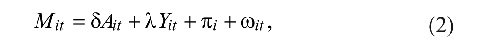
where i indexes countries and t indexes time,
A is per capita alcohol consumption, P is a real
(inflation-adjusted) alcohol price index, Y is real per capita income, and
M is a measure of age-adjusted mortality rates. Income appears directly in both
equations but also has a secondary effect in Equation 2 through the alcohol variable.
2
Model parameters are represented by
A reduced-form regression model is obtained by substituting Equation 1 for the alcohol variable in Equation 2, which yields the following:
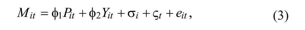
where
Deaths due to liver cirrhosis and related ailments may reflect “reservoir” effects (Edwards et al., 1994). Because many years of chronic heavy alcohol use are required for cirrhosis to develop, population-level deaths in the present time period reflect past alcohol consumption patterns. This might require a complex statistical model in which alcohol prices and income enter as lagged values in Equations 2 and 3, possibly in a distributed lag framework with unknown parameters (Cook & Tauchen, 1982; Ponicki & Gruenewald, 2006; Ramstedt, 2007). However, there are several reasons to ignore lags or at least to discount their importance. First, for a number of countries, lagged effects of consumption on population-level mortality are relatively short, on the order of 0 to 3 years (Bosetti et al., 2007; Corrao et al., 1997; Ramstedt, 2007; Zatonski et al., 2010). Second, in the reservoir model, lagged prices and lagged income are possible endogenous variables and contemporaneous values provide instrumental variables that reduce endogeneity bias. Third, log differencing of data reduces period-to-period dependence, that is, period-to-period growth rates are less dependent than data in levels as underlying trends are eliminated.
Data Sources
Data required to implement the model are from Eurostat sources for 2000-2010 (see Table 1). Supplemental data on alcohol consumption are from World Health Organization (WHO) Europe for 2000-2009. The time period was determined by comparable income data, which are not available prior to 2000. One country (Cyprus) was dropped from the EU sample in Nelson (2014) due to lack of mortality data. A few missing observations for mortality rates were obtained using a nearest-neighbor method. Table 1 displays the variable definitions, data sources, and raw data averages.
Variable Definitions and Data Sources.

Note. Index values are averages for the data period, with year 2000 = 100. For comparable country groupings, see Norstrom and Ramstedt (2005), Ramstedt (2001, 2002), and Zatonski et al. (2010). ICD-10 = Tenth Revision of the International Classification of Diseases; WHO = World Health Organization; SE = standard error.
Research Results
Male Mortality Rates, Trends for Alcohol Use, Prices, and Incomes
Table 2 displays selected values for male death rates due to alcoholic liver diseases, alcohol consumption index, alcohol price index, and index of real per capita income, normalized to year 2000 = 100. Cirrhosis mortality for males declined in 12 of 21 countries, was stable in 3 countries (i.e., change < │3.0%│), and rose in 6 countries (Finland, Ireland, Latvia, Lithuania, Sweden, United Kingdom). The rise in Finland may reflect differences in recording practices for mortality as well as recent Finnish drinking patterns (Herttua, Makela, & Martikainen, 2011; Karlsson, Makela, & Osterberg, 2010; Ramstedt, 2002). Sharp increases in mortality in several eastern European nations reflect economic changes and type of beverages consumed (Ramstedt, 2007; Zatonski et al., 2010). The index for alcohol use shows that per capita consumption declined in 9 of 21 countries, was stable in 4 countries, and rose in 8 countries. Especially sharp increases in recorded use are shown for Estonia and Latvia, reflecting important changes in economic conditions (Parna, Rahu, Helakorpi, & Tekkel, 2010; Simpura & Tigerstedt, 1999). Alcohol prices declined in 17 of 21 countries and were stable in 3 countries. Notable declines in real prices occur in Denmark (−14.2%), Finland (−11.6%), Ireland (−14.9%), Poland (−13.7%), and Sweden (−12.3%). Increases in real income occur in all countries, with especially large income gains in Estonia, Finland, Latvia, Lithuania, Poland, and Slovakia. Hence, both declining real prices and rising real incomes should increase alcohol consumption and potentially increase cirrhosis mortality in many countries.
Data Summary by Country.

Note. Alcohol use indexes are for years 2000, 2005, and 2009. For country-groups, unweighted group averages reported.
Model Specification
The dependent variable in Equation 3 is a group proportion; that is, each rate consists of a
count (nit) of the number of people in the ith country
in year t who died from alcoholic liver diseases divided by total resident
population (Nit). Hence, an observation is [Nit,
Mit,
Preliminary regression results: Alcoholic liver disease mortality rates
Results are reported in Table 3 for male mortality and total mortality rates for alcoholic liver diseases. Regression (1) in Table 3 shows preliminary results for log levels with country fixed effects, pooled cross-section weights, cluster robust standard errors, and a correction for panel data serial correlation. Without an AR(1) term, Durbin–Watson (D-W) statistics were substantially less than 2, implying positive serial correlation that inflates F statistics for overall significance and results in underestimated standard errors. The price coefficient in regression (1) is negative and statistically significant. Regression (2) shows results with time dummies substituted for the AR(1) process. Coefficient magnitudes and significance change, but a low value for D-W statistic means these results also are unreliable. In regression (3), log first-differences avoid serial correlation problems and render most data series stationary. The significant income elasticity in regression (4) is 0.455 and price elasticity is −0.722, whereas the estimated intercept in regression (3) indicates an exogenous decline in male mortality rates of −2.3% per year. Both elasticity estimates are reasonable based on earlier studies, and a positive value for income suggests an income inelastic demand for health by heavy drinkers, that is, effects of income on alcohol use dominate effects on health. Regressions (5) to (7) provide preliminary results for total mortality rates. Results are similar, except price elasticity and intercept values in regression (7) are slightly larger. Hence, preliminary regressions appear to support a negative effect of higher alcohol prices on alcoholic liver disease mortality and a positive composite income effect. 4
Regressions for Alcoholic Liver Disease Mortality Rates, 2000-2010.

Note. Sample sizes are 231 for log levels and 210 for log differences. Dependent variable in levels is the log of alcoholic liver disease mortality rate for men or total. Cluster robust standard errors in parentheses. Asterisks (*) indicate significant at the 95% confidence level or better. Regressions (1) and (5) employ GLS cross-section weights. D-W is the Durbin–Watson statistic for serial correlation. Unit root tests did not reject the null of non-stationarity for 17 of 21 log-level mortality data series. Robust results were obtained using Stata subroutine msregress for MS-estimator for panel data. None of the predicted values in levels are negative. OLS = ordinary least squares; AR(1) = first-order autoregressive term; GLS = generalized least-squares.
Robust-regression results: Alcoholic liver disease mortality rates
Robust regressions address issues of outliers and influential data points. Outliers in mortality data can arise due to inaccuracies in reporting methods, clusters of outcomes due to reservoir effects, unusual age or gender cohort effects, and other sampling peculiarities. Large residuals affect OLS estimation and prediction, especially the estimated intercept. Large residuals, however, do not necessarily imply unusual observations for the set of explanatory variables, that is, observations are outlying in the vertical or y dimension only (Verardi & Croux, 2009). Influential data points are due to extreme values of explanatory variables, such as unusual circumstances that affect alcohol prices or consumer incomes (economic liberalization, recessions, labor strikes, weather, large data errors, etc.). These observations are said to have “high leverage,” meaning that OLS slope coefficients are influenced by observations that are far from the true regression plane in the horizontal or x dimension. Observations that are both outliers and of high leverage exert influence on slopes and intercept of the model. Although deletion of outliers and influential data points is possible, these points tend to be masked by OLS panel methods and traditional diagnostics may not be reliable (Bramati & Croux, 2007; Verardi & Croux, 2009). Furthermore, discarding of data is always suspect. A number of robust-regression methods have been proposed to deal with these issues, which down-weight cases with large residuals. The M-estimator due to Huber (1964) is an iteratively weighted OLS estimator, but it deals only with a problem of vertical outliers. The S-estimator and MM-estimator address bad leverage points and outliers, but these methods cannot handle categorical dummy variables (Verardi & Croux, 2009). As a consequence, Maronna and Yohai (2000) propose a combination of M- and S-estimators, which was generalized to panel data econometrics by Bramati and Croux (2007). The MS-estimator uses a highly efficient M-estimator for categorical dummy variables, which do not contain leverage points. The S-estimator is then used for continuous variables, which is robust with respect to leverage points.
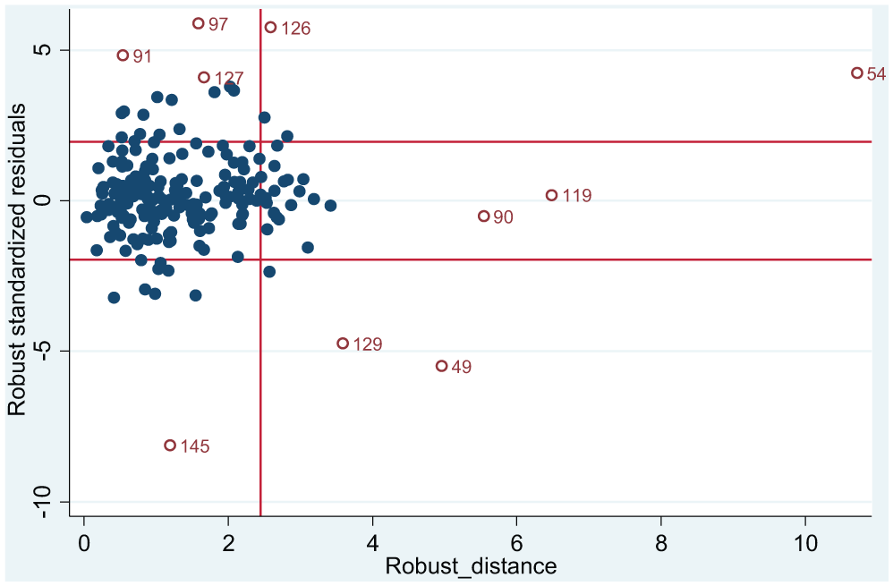
Regressions (4) and (8) in Table 3 show results for reduced-form mortality model obtained using the MS-estimator (Stata msregress subroutine). In regression (4), slope coefficients for price and income are not statistically significant and their magnitudes are reduced substantially. The intercept has the same value as regression (2), although it is no longer significant. Regression (8) reports similar results for total mortality, except the intercept is significant with a value of −0.039. Hence, results obtained using robust regressions indicate that alcohol prices and income are not reliable predictors of mortality rates due to liver diseases. Robust corrections for outliers are shown here to be important for empirical results for alcohol prices, income, and mortality rates due to liver cirrhosis. These results are illustrated in Figures 1 and 2, which display diagnostic plots of robust standardized residuals (measure of vertical outlyingness with respect to fitted regression plane) versus robust distances (measure of horizontal outlyingness of explanatory variables). Two horizontal lines in the figures are used to flag outlying residuals in vertical directions (standardized residuals greater than |2.25|). There are 20 vertical outliers in Figure 1 and 22 in Figure 2. The vertical line flags outliers in the horizontal direction. There are 41 horizontal outliers in Figure 1 and 44 in Figure 2. Large outliers in the vertical direction can be due to unusually large or small observations for the dependent variable, so observed growth rates are too large or small relative to other values. Extreme vertical outliers for male mortality in Figure 1 are observations 91 (Ireland, year 2001), 92 (Ireland, 2002), 94 (Ireland, 2004), 97 (Ireland, 2007), 117 (Latvia, 2007), 126 (Lithuania, 2006), 144 (Norway, 2004), and 145 (Norway, 2005). Extreme leverage points in the horizontal direction are observations 49 (Estonia, 2009) and 54 (Finland, 2004). Other residuals are possible “good leverage points” (outliers in horizontal direction only) such as observations 90 (Greece, 2010) and 119 (Latvia, 2009). Figure 2 shows fewer extreme vertical outliers for total mortality, suggesting reporting of these rates may be more reliable. New outliers in Figure 2 are observations 127 (Lithuania, 2007) and 129 (Lithuania, 2009).

Diagnostic plot for male mortality.
Diagnostic plot for total mortality.
Discussion
Empirical results in this article have several important implications for modeling of alcohol-related harms and for alcohol policy. Panel data are widely used in health economics and related areas, but attention to robustness has focused on standard errors and corrections for clustering. As defined by Huber (1981), robustness means that results for a regression model are insensitive to small deviations from assumptions the model imposes on data (unbiased, efficient, stationary, normality, etc.). Although OLS results are robust with respect to corrections for non-stationary data, as illustrated by regressions (3) and (7), this result did not carryover to distributional robustness and impacts of outliers or influential data points. As shown here, separated data points have a strong influence on OLS results as demonstrated by regressions (4) and (8) in Table 3. This outcome occurs for both the price variable and income variable, with the latter case suggesting that opposing income effects in Equations 1 and 2 tend to cancel out. Graphs indicate possible uniqueness of data for Ireland, but other influential data points are possible for Finland, Lithuania, and other countries. More generally, robust treatment of a small fraction of the sample of 210 observations produced marked changes in empirical results.
The results suggest that earlier reviews of alcohol-related mortality are based on studies that do not attend sufficiently to data-related issues. For example, Elder et al. (2010) review five studies of alcohol prices and deaths from liver cirrhosis, including several studies using panel data. They note substantial differences in estimated strength of the relationship, and suggest this may be due to methodological differences. Results reported here indicate that other data issues may be equally important, because earlier studies did not attend to outliers or influential data points. Nelson (2013a) reviews nine cirrhosis mortality studies, including seven that use panel data for the United States or Organization for Economic Co-Operation and Development (OECD). Results again tend to be sensitive to model specification, but none of the studies corrected for either non-stationary data or outliers. Nelson (2013a) concludes that the relationship between alcohol prices and cirrhosis mortality was insignificant or at least uncertain given current evidence. A re-examination of data used in these studies would be a useful follow-up to the present article. Greater use of individual survey data also mightcircumvent some data issues associated with small samples.
Much of present-day alcohol policy is based on a population-level model that follows from work by Rose (1992) and Skog (1985). Briefly, harmful alcohol consumption is systematically related to average or population-level consumption in a society, including alcohol consumption by light or moderate drinkers (Babor et al., 2010). However, given empirical evidence in the present article, the economic basis for a harms–price relationship is less certain, at least for aggregate data. Although policy statements, such as those contained in Anderson et al. (2009) and Babor et al. (2010), make every attempt to formulate evidence-based policies, such policy statements are only as good or reliable as underlying empirical studies. When population-level studies are faulty or suspect, a conservative approach to public policy is in order. As shown here, the research base for cirrhosis mortality is not as strong as claimed when it comes to economic evidence for prices or incomes (see also Nelson, 2013a, 2015, for supporting evidence).
Conclusion
This study estimates a reduced-form model for mortality rates due to alcoholic liver diseases. The pooled-longitudinal or panel data sample covers the years 2000-2010 for 21 countries that are members of the EU. Basic explanatory variables are an index of real alcohol prices and real per capita disposable income. In the reduced-form equation for mortality rates, price affects mortality indirectly through the demand for alcohol, whereas income has potential direct and indirect effects. Country and time fixed effects are used to control for other factors that influence alcohol consumption and alcohol-related mortality, including unobservables. To ensure stationary data, a log-difference linear model is used for statistical estimation of group probabilities. Empirical results for price are sensitive to weighting of outlier observations, suggesting that price results in past studies and surveys are possibly idiosyncratic and not causal in nature. Empirical results for income suggest that direct and indirect forces on alcohol demand and health tend to be offsetting. Numerous econometric results are shown to be “fragile” or highly dependent on data sample or model specification (Kennedy, 2008; Woodward, 2006). Robust regressions that down-weight outliers indicate that alcohol prices do not affect mortality rates, which supports survey results reported in Nelson (2013a). Empirical results in the present study thus do not support broad price-based approaches to population-level alcohol policy.
Footnotes
Declaration of Conflicting Interests
This paper presents the work product, findings, viewpoints, and conclusions solely of the author. The views expressed are not necessarily those of IARD or any of IARD’s sponsoring companies.
Funding
Research leading to this paper was supported in part by the International Alliance for Responsible Drinking, Washington, DC.