Sage Journals: Discover world-class research

Abstract

In this study, we use double-robust estimators (i.e., inverse probability weighting and inverse probability weighting with regression adjustment) to quantify the effect of adopting climate-adaptive improved sorghum varieties on household and women dietary diversity scores in Tanzania. The two indicators, respectively, measure access to broader food groups and micronutrient and macronutrient availability among children and women of reproductive age. The selection of sample households was through a multistage sampling technique, and the population was all households in the sorghum-producing regions of Central, Northern, and Northwestern Tanzania. Before data collection, enumerators took part in a 1-week training workshop and later collected data from 822 respondents using a structured questionnaire. The main results from the study show that the adoption of improved sorghum seeds has a positive effect on both household and women dietary diversity scores. Access to quality food groups improves nutritional status, food security adequacy, and general welfare of small-scale farmers in developing countries. Agricultural projects that enhance access to improved seeds are, therefore, likely to generate a positive and sustainable effect on food security and poverty alleviation in sorghum-producing regions of Tanzania.

Keywords

dietary diversity doubly robust improved sorghum varieties inverse probability treatment weighting Tanzania weighted regression

Introduction

According to Dalton and Zereyesus (2013), sorghum is one of the climate change–ready crops grown by the world’s most vulnerable household groups. The sorghum crop has a high potential of improving the livelihood of small-scale farmers in the semiarid tropics of Africa, the region prone to frequent droughts and high incidences of food insecurity. Regional research and extension programs aim to increase both the production and productivity of the sorghum production sector to increase food access and income of sorghum producers. In Tanzania, the colonial government started the sorghum and millet improvement program in the early 1930s. Since then, as described in Mgonja et al. (2005), steps have been taken to develop improved sorghum varieties (ISVs) that are high yielding and tolerant to drought. In the 1970s, Tanzania started a sorghum selective breeding program in collaboration with the Southern Africa Development Community (SADC) and the International Crop Research Center for Semi-Arid Tropics (ICRISAT). The main goal was developing new ISVs with desirable characteristics. The efforts resulted in the release of several ISVs, including Tegemeo (1978), Pato (1997), Macia (1998), Wahi and Hakika (2000), and Mtama 1 and Sila (2008). Supplemental Appendix 1 presents the characteristics of these varieties and the history of sorghum research and development in Tanzania. For more details, see Kilimo (2008) and Kanyeka et al. (2007). However, no studies assess the effect of adopting these varieties on farmers’ welfare.

One of the core goals of most agricultural development programs is improvement in the food security of small-scale farmers. Accordingly, in the impact assessment literature, most studies use food security as measures of welfare or well-being. Studies such as Kassie et al. (2011), Amare et al. (2012), Asfaw et al. (2012), Shiferaw et al. (2014), Mathenge et al. (2014), Kabunga et al. (2014), Mason and Smale (2013), Smale and Mason (2014), and Khonje et al. (2015) try to estimate the effect of adopting improved maize, wheat, groundnuts, pigeon-peas, and other crops on different indicators of farmers’ welfare, including food security. Apart from Smale et al. (2018), who document the effect of ISVs in Mali, there are limited studies that focus on ISVs, especially in the East and Southern African region. Available studies use income and consumption expenditure as measures of welfare. However, these variables are difficult to quantify when record-keeping is not standard across the sample. Small-scale farmers are also both producers and consumers, and most transactions are outside of formal markets. Valuing all sources of income or expenditures (through recall) is prone to measurement errors, as discussed by Ellis (1998) and Chen and Ravallion (2007). Mahlberg and Obersteiner (2001) and World Food Program (2005) present the household dietary diversity score (HDDS) and the women’s dietary diversity score (WDDS) as an easily quantifiable alternative measure of food security and therefore farmers’ well-being.

The 1996 World Food Summit agreed that food security has three critical components (Population Council, 1996): availability, access, and use. Food availability addresses the supply side of food security, determined by the level of food production, stock levels, and net trade. As a measure of nutritional status, use refers to the individual’s biological ability to make use of food for a productive life. Household food access, in the context of food security, is the ability to get enough quality and quantity of food to meet all household members’ nutritional requirements for productive lives. However, food security is an evolving concept (Jones et al., 2013) about issues of terminology, measurement, and validation. Therefore, no one indicator can concomitantly capture all three components of food security (Webb et al., 2006). This article emanates from the main study that documents profitability and adoption of ISVs in Tanzania. Detailed information on profitability has been reported in Kaliba et al. (2017), and a detailed analysis of factors affecting adoption is published in Kaliba et al. (2018).

As reported by Kendall et al. (1996) and Operations Evaluation Department (2011), poverty (a critical indicator of well-being) undoubtedly causes food insecurity. However, the lack of adequate and proper nutrition itself is an underlying cause of poverty. The interwoven nature of poverty and food security justifies using HDDS and WDDS as measures of well-being (Zhao et al., 2017). According to Mahlberg and Obersteiner (2001), Arimond and Ruel (2004), and Martin-Prével et al. (2015), HDDS represents the ability of a family to access food groups that meet all household members’ nutritional requirements. The HDDS is, therefore, a useful tool for measuring household food access and adequacy, the critical dimensions of food security, and well-being in developing countries. Arimond and Ruel (2004), Swindale and Bilinsky (2006), and Luckett et al. (2015) show a high and positive correlation between HDDS and other nutritional factors such as the availability of high-quality proteins that positively influence food security adequacy.

The WDDS reflects one crucial dimension of diet quality—macronutrient and micronutrient adequacy (Gernand et al., 2016)—among children and women of reproductive age (15–45 years). Zhao et al. (2017) validate WDDS as an indicator for evaluating micronutrient inadequacy in Chinese children. Kennedy et al. (2013), Food and Agriculture Organization of the United Nations (FAO, 2014), and Becquey et al. (2010) also indicate that children and women who have access to various diet items have a higher likelihood of meeting both micronutrient and macronutrient requirement. As no single food has all essential micronutrients and macronutrients, a balanced and varied diet is necessary for adequate intake of these nutrients. Hatloy et al. (2000), Gina et al. (2007), Faber et al. (2017), Chakona and Shackleton (2017), and Sibhatu and Qaim (2018) reveal that apart from focusing on food access and quality, HDDS and WDDS are positively associated with wealth or general welfare at the household level. In their studies, Arimond and Ruel (2004), and FAO (2014) also concluded that the two indicators are positively related to household food security and other poverty indicators, such as income and households’ food expenditure levels. Although food security may not encapsulate all aspects of poverty, the inability of households to access enough food for a productive and healthy life is an essential part of households’ socioeconomic status (Ravallion and Chen, 1997). In summary, dietary diversity is a good proxy of food security and the general welfare. They are useful for monitoring changes and effect, especially when data on traditional money-metric measures are unavailable.

Swindale and Bilinsky (2006), Kennedy et al. (2007), and FAO (2014) give a detailed account of quantifying the HDDS and WDDS at the individual or household level. The process allows itemizing food items consumed over the last 24 hr. Supplemental Appendix 2 lists the food groups. A new method uses Minimum Dietary Diversity–Women (MDD-W) to assess the micronutrient adequacy of women’s diets. The new indicator reflects (Martin-Prével et al., 2015) consumption of at least five of 10 food groups. The tool was not available during data collection for this study. The estimate of HDDS is from a set of 12 food groups, including cereals; fish and seafood; root and tubers; pulses/legumes/nuts, vegetables; milk and milk products; fruits, oil, and fats; meat, poultry, and offal; sugar and honey; eggs; and other food groups. The HDDS ranges from 0 to 12, and a score of less than 5 shows low dietary diversity or food insecurity (Arimond & Ruel, 2004). Nine food groups are used to construct the WDDS and include grains; white roots and tubers, and plantains; pulses (beans, peas, and lentils); nuts and seeds; dairy and dairy products; meat, poultry, and fish; eggs; dark green leafy vegetables; and, other vitamin A–rich fruits and vegetables. As the calculation of WDDS involves nine food groups, the score should range from 0 to 9, and a score of less than or equal to 4 shows macronutrient and micronutrient inadequacy (Huang et al., 2018).

As summarized by Webb et al. (2006) and Kennedy et al. (2013), the use of HDDS and WDDS as measures of food access and quality has two main advantages. The data collection is not time-consuming, is inexpensive, and does not require specialized professionals (e.g., nurses) for data collection, analysis, and interpretation. Carefully trained extension agents could get the technical skills required to collect and analyze the data on both HDDS and WDDS. Savy et al. (2005), Kennedy et al. (2007), and Luckett et al. (2015) underscore the importance of these indicators in terms of minimizing measurement errors when using trained enumerators. Becquey et al. (2010) emphasize that the questions used to collect the data are not complicated, not intrusive, and not burdensome. The United States extensively uses the 24-hr dietary recall technique (Thompson & Byers, 1994) due to its speed and ease of administration (Nelson & Bingham, 1997). The Demographic and Health Surveys (https://dhsprogram.com/) have used the 24-hr dietary recall approach for more than two decades, and the approach is also recommended by the European Food Safety Authority (2009). See supplemental Appendix 2 for the part of the survey instrument used to collect the data on the two indicators, and for details, see FAO (2014).

In Tanzania, sorghum is both a cash and food crop. Theoretically, the adoption of ISVs may induce the consumption of various food items through two pathways: an increase in income and unlocking the land and other resources to produce other food crops. Increased production and productivity create opportunities to improve farm income by selling surpluses. Excess production allows farmers to take part in the food and crop markets that increase food security as explained in Koppmair et al. (2017) and Jones (2017). Increased productivity also allows farmers to use fewer resources to produce more sorghum. The saved production inputs are for producing other crops that generate more income and broaden access to healthier and diverse food groups. See, for example, Smale et al. (2015) and Ecker (2018).

When conducting an impact assessment using observational data, Shadish et al. (2008) emphasize the importance of adjusting for self-selection and confounding effects. We, therefore, adapted the inverse probability weighting (IPW) and the inverse probability weighting with regression adjustment (IPWRA) for estimating the effect of adopting ISVs. The two techniques allow estimating consistent and unbiased results as explained in Austin et al. (2007), Wooldridge (2007), and Linden (2017). The contributions of this study are as follows. Explaining the complex linkage between improved seed adoption and food access adds the required literature on sorghum effect assessment for the Eastern and Southern African region. Also, showing the effect of ISVs encourages governments, policymakers, and the private sector to increase funding for agricultural research and extension systems that support small-scale sorghum producers. Results from effect studies also help the internal learning processes by showing changes that enhance the probability of adoption and capturing the linkages between innovations and sustainable agricultural development.

The use of HDDS and WDDS as measures of food access and food quality that are essential measures of food security and general welfare allows the study to be easily replicable. Importantly, most studies that use inference models are common in disciplines other than agriculture and are presented in unclear language for applied agricultural economists. In this study, we try to use familiar words in agricultural technology adoption and impact assessment literature for replication purposes. We organize the rest of the article as follows. In the following section, we summarize the history of sorghum research and development in Tanzania. We use section “A Conceptual and Empirical Framework” to, respectively, discuss the source of data, analytical methods adopted in this study, and the covariates used in the study. In sections “Results and Discussion” and “Conclusion,” we, respectively, present key findings and the policy implications.

Source of Data

The data for this study are from Central, Northern, and Northwestern Tanzania. The survey included the main sorghum-producing regions of Dodoma, Manyara, Kilimanjaro, Singida, and Shinyanga. The enumerators were extension agents working in these regions, supervised by sorghum research scientists from Selian Agricultural Research Institute (SARI) in Arusha and Homboro Agricultural Research Institute (HARI) in Dodoma. These enumerators took part in a 1-week training workshop on data collection using a structured questionnaire. The trainers were scientists from ICRISAT in Nairobi, Kenya, and the principal author. The pretesting of the clarity of questions in the questionnaire was by using 30 randomly selected samples of sorghum producers in Singida Rural and Rombo Districts (Map 1). The responses and gained experience from pretesting helped to set the final questions.

Map 1.

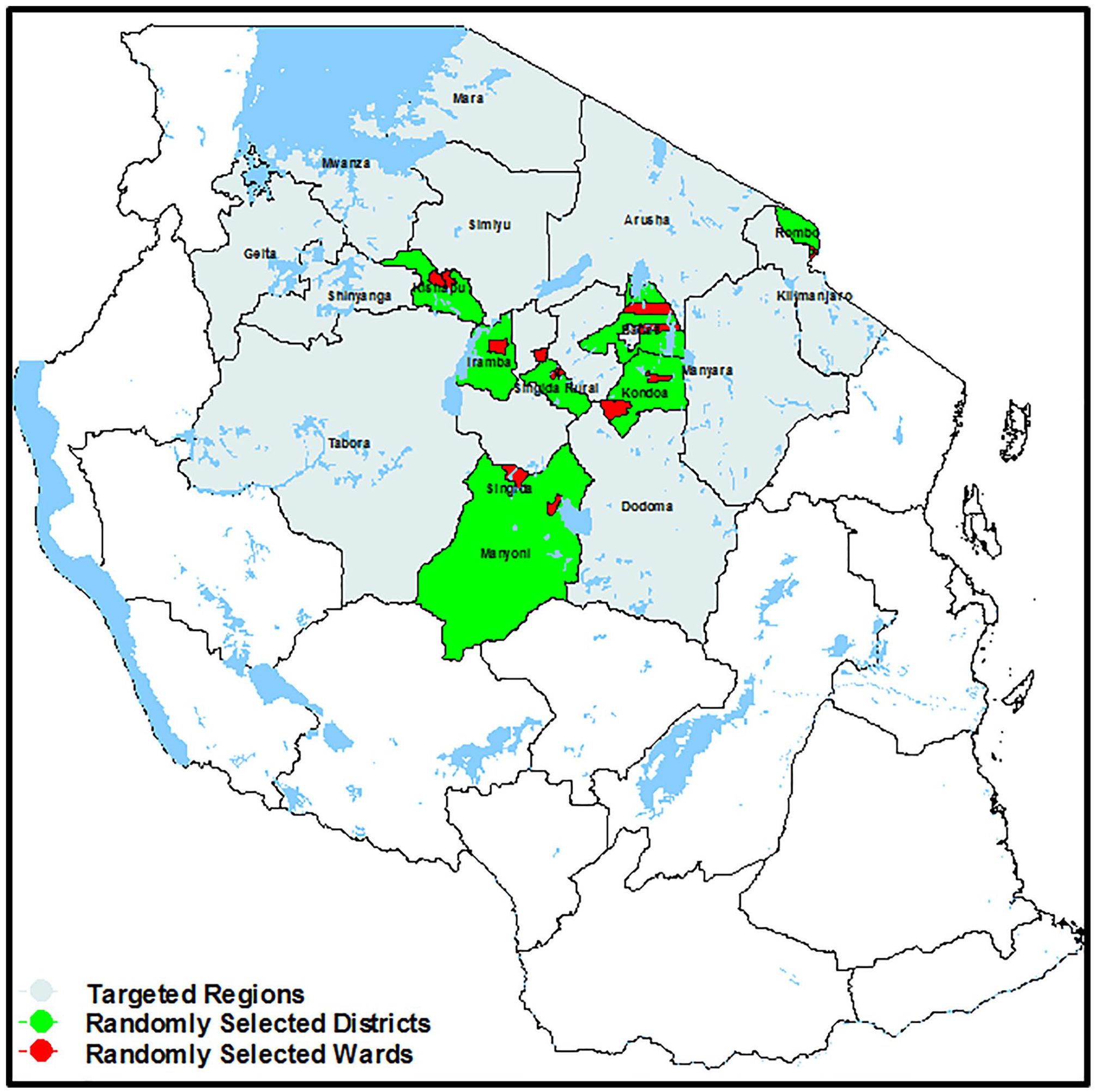
Location of targeted regions and randomly selected districts and wards.

Tanzania is administratively divided into Regions, Districts, Ward, and Villages. A region constitutes more than three districts, a district constitutes more than five wards, a ward constitutes more than five villages, and the village is the lowest administrative unit. The sample households were selected using a multistage sampling design (Etikan & Bala, 2017), that is, Regions, Districts, Wards, and Villages from the primary sorghum farming system in Central, Northern, and Northwestern Tanzania (Map 1). The target area produces more than 70% of the national sorghum. The randomly selected regions were Dodoma, Manyara, Kilimanjaro, Singida, and Shinyanga. From these regions, we randomly selected seven districts to take part in the study. The districts included Iramba, Singida Rural, and Manyoni districts (Singida Region), Kondoa District (Dodoma Region), Babati District (Manyara Region), Rombo District (Kilimanjaro Region), and Kishapu District (Shinyanga Region) (see Map 1). We then randomly selected two Wards per selected District and one Village per selected Ward. For statistical purposes, about 50 randomly selected households per village took part in the survey. Previously trained enumerators interviewed 822 respondents using a structured questionnaire. In the sample, 505 respondents were from adopters of ISVs (61.44%), and 317 respondents were from nonadopter group (38.56%). Based on the type of questions in each section, the respondents were knowledgeable or informed members of the sample households.

The survey instrument had several parts to collect data on the geolocation of the sample households, household and farm characteristics, farm inputs and outputs, harvesting, processing, transportation, marketing, and access to services offered by government and nongovernmental organizations. To estimate the HDDS and WDDS, we adapted the food access questions from Swindale and Bilinsky (2006) as modified in FAO (2014). The questions asked about consumed food groups listed in supplemental Appendix 1 by members of households in the last 24 hr during breakfast, lunch, dinner, and in-between snacks.

During data collection and entry, we instituted three measures to ensure data quality. First, we grouped enumerators into seven individuals: six enumerators and a supervisor. All enumerators had a Diploma in Crop Production, and they were working in the region as extension agents for more than 5 years. All supervisors were research scientists with graduate-level training in Crop Production or Agricultural Economics and had experience in conducting farm-level surveys through other projects implemented by their respective research institutions. After administering the questionnaire, the enumerator and the supervisor reviewed the responses before leaving the respondent household to ensure clarity and completeness of the answers. The supervisor asked additional questions if more information and explanations were needed. Second, after administering the questionnaire, the responses were entered into an SPSS spreadsheet by the supervisor with the help of enumerators. Third, the data scientists at SARI and ICRISAT, and the principal author rechecked the combined data from the survey groups (questionnaire by questionnaire) to ensure the accuracy and consistency of data. We completed the study in about 6 months (from the training workshop, data collection, and data entry and cleaning).

A Conceptual and Empirical Framework

Dehejia and Wahba (1999), Kang and Schafer (2007), and Skelly et al. (2012) discuss the challenge of estimating the effect of an intervention using observational data while accounting for putative confounding factors and self-selection bias. After releasing ISVs, the adoption processes occur naturally, and as the adoption process is not random, adopters and nonadopters tend to differ systematically. Adapted from the causal inference model of Rosenbaum and Rubin (1983, 1985), the IPW and IPWRA estimators allow adjusting for both self-selection and confounding effects. Bang and Robins (2005), Robins et al. (2007), Wooldridge (2002, 2007), and Funk et al. (2011) present the justification and statistical properties of these estimators. Glynn and Quinn (2010), Funk et al. (2011), and Uysal (2015) present the advantages and disadvantages of each approach.

Formally, let D_it(T_i) represent an indicator of adoption status and $D_{i t}^{*} (T_{i})$ a latent variable for adoption status, where T_i is the binary variable such that T_i = t, and t ∈ = {1,0} represents, respectively, adoption and nonadoption statuses. For each household i (i = 1,. . ., N) in the sample (where N is the sample size), we observe a triple (Y_i, T_i, Z_i) such that Y_i is the welfare measure (i.e., HDDS or WDDS), T_i is the binary adoption status variable described above, and Z_i represents the matrix of covariates that influence the welfare measures. Following Caliendo and Kopeinig (2008) and Abebe and Bekele (2015), the adoption equation and the weighted least squares regression to estimate the effect of adoption using IPW and IPWRA are as follows:

Step 1: Adoption equation

D_{i t}^{*} (T_{i}) = X_{i} γ + υ_{i} {\begin{cases} 1, i f t_{i} = 1 \\ 0, O t h e r w i s e . \end{cases}

(1)

Step 2: Welfare equation

\begin{array}{l} \underset{α_{1}, β_{1}}{m i n} \sum_{i = 1}^{N} (y_{i} - α_{1} - β_{1} Z_{i}) W_{1} i f D_{i t} (t = 1) \\ + \underset{α_{0}, β_{0}}{m i n} \sum_{i = 1}^{N} (y_{i} - α_{0} - β_{0} Z_{i}) W_{0} i f D_{i t} (t = 0) \end{array}

(2)

Equivalently, \underset{α_{t}, β_{t}}{m i n} \sum_{i = 1}^{N} W_{t} {(y_{i} - {\hat{y}}_{i})}^{2}, t \in = {1, 0} .

In Equations 1 and 2, $X_{i}$ is the matrix of covariates that influence adoption, $y_{i}$ is the observed welfare measure for the ith household, ${\hat{y}}_{i}$ is the predicted (or calculated) value of the welfare measure for the ith household, and γ, α_i, and β_i are vectors of model parameters. The variables W₁ and W₀ or W_t in Equation 2 are right weights for adopters and nonadopters, respectively. These weights are from the inverse of the estimated propensity score, and υ_i is the random error term. All other variables are explained above. $W_{t}$ is the weighting factor and is equal to 1 for unweighted least square regression. The weights in Equation 2 allow attaining essential characteristics of a randomized controlled trial and meeting all assumptions on common-support and ignorability when using observation data (Cattaneo, 2000; Austin, 2009, 2011). Recent applications of this weighted model include Awel and Azomahou (2014) and Smale et al. (2018). For IPW, Z_i includes only the adoption status variable, and for IPWRA, Z_i consists of all variables influencing welfare, including a binary variable standing for the adoption status. If the weighting factor enters Equation 1 as inverse of the propensity scores, the estimated coefficient on the adoption status stands for the effect of adoption on welfare.

Results from Equation 2 are for estimating three common estimands: the average treatment effect for the treated (ATT) or the effect among adopters of ISVs; the average treatment effect (ATE) for the entire sample; and the average treatment effect for the controls (ATC) or the potential effect among nonadopters. Lee et al. (2011) and Uysal (2015) discuss how to estimate and apply right weights ( $W_{t}$ ) for estimating each measure. From the policy perspective, although the ATE is useful for determining how adoption has affected a group of adopters in the sample, ATT shows sample average adoption effect for the subsample of adopters. The ATC shows a potential average adoption effect for nonadopters. Heckman and Vytlacil (2007) and Guo and Fraser (2010) relate ATE to the intention-to-treat (adoption) concept in the randomized trial or the average benefit of adoption among all households. The ATE does not show that all groups of farmers benefited from the uptake of ISVs (Wooldridge, 2007). It neglects the distribution effect of adoption. The ATT and ATC are particularly useful when heterogeneity among the sample is essential, and the projection of potential welfare among nonadopters is also critical.

In terms of covariates to include in Equations 1 and 2, Angrist and Pischke (2009) and Stuart (2010) argue that the variables in matrix Z should influence both adoption status and welfare of farmers, but should not be affected by the adoption decision. For example, although farmer and farm characteristics influence both adoption decisions and well-being of farmers, institutional support systems directly influence adoption decisions and not the welfare of farmers. Suggestion is not to include institutional support variables in the welfare equation. Holden et al. (2001), Doss et al. (2003), Thomson et al. (2014), Ainembabazi and Mugisha (2014), Mwangi and Kariuki (2015), Kebede and Tadesse (2015), and several other authors present the covariates to include in the adoption and welfare equations and associated rationales not replicated here. Supplemental Appendix 3 presents the definitions and explanations for each covariate included in this study.

The covariates included in the model represented farmer characteristics including the quantity of available labor, education of household head, weighted mean household-level literacy index, dependency ratio, the weighted mean age for adults, marital status of household head, the gender of household head, and a log of total wealth. For institutional support systems, we include variables measuring the quality of extension services received by the farmers, availability of credit, market participation (through selling surplus crop), and household participation in research and extension activities. To capture the general built environment in which the farmer operates, we constructed a built environment index using data envelopment analysis (DEA). As defined in Farrell (1957) and Charnes et al. (1978), DEA is a linear programming technique for identifying the most efficient unit where the benchmark is the best practice in the sample. Mahlberg and Obersteiner (2001) and Despotis (2005) used DEA to develop human development index. Authors such as Somarriba and Pena (2009), Sharpe and Andrews (2010), and Sisay et al. (2015) used the technique for constructing the quality of life and economic well-being of communities and productive efficiency of small farms. When all inputs are binary, the index is estimated by imposing a free disposability hull with no convexity assumption. The DEA allowed aggregating different binary variables, showing the availability of agricultural support services such as extension and veterinary services, and agricultural input suppliers. The constructed built environment indicator varied from 1 (remarkably high support) to 0 (no support). Regional dummy variables (i.e., Singida, Kilimanjaro, Manyara, Shinyanga, and Dodoma) were also included in the model to represent geolocation, resource base, production potential, farming conditions across regions, and specific attributes of the adopted varieties. The analysis was conducted in the R environment (R Core Team, 2019) using a Benchmarking package (Bogetoft & Otto, 2018) for DEA and survey package (Lumley, 2018) for weighted regression analysis.

Results and Discussion

Summary Statistics of Estimated HDDS and WDDS From the Survey

The summary statistics of covariates included in the welfare model and the results of the pairwise comparison of food diversity indicators across regions are shown in Table 1. The comparison is by using the t-test with pooled standard deviation. The overall results in Table 1 show a statistically significant difference between the adopter and the nonadopter at more than .1 probability level. The average HDDS was, respectively, 5.364 and 4.568 among adopters and nonadopters, with standard deviations of 2.137 and 1.987, respectively, for the entire sample. Also, the average HDDS in all regions were higher among adopters compared with nonadopters, implying that adopters were diverse food-adequate compared with nonadopters. Except for Dodoma and Shinyanga regions, the standard deviation of adopters was large and statistically significant when compared with the standard deviation of nonadopters, showing evidence of widely distributed scores among adopters in comparison with nonadopters. The estimated mean HDDS are comparable to other studies in Tanzania. For example, at 95% confidence level, Ntwenya et al. (2017) estimated HDDS for Kilosa District (Eastern Tanzania) to be 4.7 [4.5, 5.0] during the rainy season and 5.9 [5.7, 6.1] during the harvest season. Mbwana et al. (2016) also estimated the mean HDDS to be 4.7 for the Morogoro Region in Eastern Tanzania and 4.1 for the Dodoma Region in Central Tanzania.

Table 1.

Summary Statistics of Indicators of Dietary Diversity by Regions.

Region	Diverse food	Nonadopters		Adopters		p value
Region	Adequacy	M	SD	M	SD	p value
Household dietary diversity scores
Dodoma	51.96%	4.725	1.826	6.145	1.726	.001***
Kilimanjaro	77.19%	6.000	1.744	6.968	2.575	.098*
Manyara	50.91%	4.447	1.943	5.635	2.105	.003***
Shinyanga	25.42%	3.945	1.840	4.556	1.702	.065*
Singida	45.98%	4.544	2.028	5.140	2.126	.005***
Pooled Sample	50.29%	4.568	1.987	5.364	2.137	.001***
Women dietary diversity scores
Dodoma	3.92%	1.675	1.095	2.871	0.932	.001***
Kilimanjaro	10.53%	2.462	1.104	3.548	1.567	.003***
Manyara	100%	1.532	0.905	2.000	0.803	.006***
Shinyanga	100%	1.527	1.103	1.667	0.762	.433
Singida	2.92%	1.779	1.167	2.392	1.220	.001***
Pooled Sample	3.49%	1.741	1.126	2.382	1.200	.003***

Significant at 10% level. **Significant at 5% level. ***Significant at 1% level.

The results in Table 1 also show that except for the Shinyanga Region, WDDS of adopters and nonadopters were statistically different at more than 10% level. The average scores for the pooled sample were, respectively, 2.382 and 1.741 for adopters and nonadopters, and the standard deviations were, respectively, 1.2 and 1.26. Although the WDDS among nonadopters were lower and more variable compared with the distribution of WDDS among adopters, on average, all regions exhibited micronutrient and macronutrient inadequacy for both adopters and nonadopters. In both cases, sample households in Kilimanjaro had the highest HDDS and WDDS, and sample households in Shinyanga had the lowest scores.

Compared with other studies, Chakona and Shackleton (2017), using a survey instrument that measured MDD-W, estimated the mean scores of 3.78 for Richards Bay, 3.21 for Dundee, and 3.36 for Harrismith townships in Southern Africa. All three townships signified micronutrient and macronutrient inadequacy for children and women of reproductive age. Smale et al. (2015) found that women living in households that adopted improved maize seeds in Zambia had access to broader food items, but the score was below the threshold of micronutrient and macronutrient inadequacy. Keding et al. (2012) reported comparable results about the adoption of improved vegetable seeds in rural Tanzania.

Focusing on the distribution of HDDS at the regional level, the results in Table 1 show that 77.19% of households in Kilimanjaro were diverse food-adequate, the highest score in the sample. The lowest percentage was in the Shinyanga Region where 25.42% of households were food-adequate. Analogous results were 51.96%, 50.91%, and 45.98% of households in the Dodoma, Manyara, and Singida regions, respectively. In terms of WDDS and from Table 1, all sample households in Manyara and Shinyanga regions were in the micronutrient and macronutrient inadequacy class. Only 10.53% of sample households in the Kilimanjaro Region, 3.92% in the Dodoma Region, and 2.99% in the Singida Region reported micronutrient and macronutrient adequacy with an implication that very few households have access to different food items that ensure nutrient adequacy for children and women of reproductive age in the study area. A study by Huang et al. (2018) also supports the evidence that limited numbers of households in the Dodoma Region meet macronutrient and micronutrient demand of children and women of reproductive age. Although using a different method to estimate food adequacy, Kinabo et al. (2016) concluded that women undernutrition in Tanzania was attributable to poorly diversified diets and macronutrient and micronutrient inadequacy.

Higher food diversity in Kilimanjaro is associated with the regional staple food, banana. The region is also suitable for growing other crops such as legumes and avocado, fruits, and leafy vegetables. They raise dairy cattle and small stocks for meat and milk consumption. As discussed in Faber et al. (2017), households with access to these kinds of food items are more likely to have access to more diverse food items. In the Shinyanga Region, the staple food has historically been “ugali,” a stiff porridge made by mixing maize flour (cornmeal) or sorghum or finger millet or cassava powder with boiling water and served mainly with vegetable soups. The meal is starchy with high calories and tends to lack high-protein food items and fruits. According to Kinabo et al. (2016) and Ochieng et al. (2017), when households’ staple food depends on cereals, dietary diversity is typically low as crops and livestock products are usually sold to stock the staples to the detriment of dietary diversity.

Propensity Score Diagnosis

Propensity score diagnosis or analysis is for examining whether the propensity score model or the adoption equation has been correctly specified. The diagnosis is for proving whether the covariates of farmers with the same propensity score have the same distribution among adopters and nonadopters. Standardized mean difference (SMD) and distributional analysis are the most used statistics to examine the balance of covariate distribution between the two groups (Greifer, 2019; Stuart et al., 2013). Because SMD is independent of the unit of measurement, it allows comparison among variables with different units. Before using the SMD, side-by-side comparisons of the density plots of adopters and nonadopters allow testing for both the ignorability and common-support assumptions, as shown in Figure 1. The density plots of the estimated propensity score among adopters and nonadopters indicate a substantial overlap between the two groups (left part of Figure 1). Also, the densities do not have too much mass around 0 or 1 (right part of Figure 1), which could lead to the violation of the common-support assumption.

Figure 1.

Distribution of propensity scores among adopters and nonadopters.

Based on the distribution of density plots in Figure 1, the estimated mean propensity score for the adopter group was 0.6721, and the interval was [0.0558, 0.9685] at a 95% confidence level. The mean propensity score for the nonadopter group was 0.5223, and the interval was [0.0066, 0.937] at a 95% confidence level. Using the minima and maxima criterion, the interval for the regional of common-support is [0.0558, 0.937]. The common-support is, therefore, truncated at 0.0558 to the left and 0.937 to the right. Because there are more adopters than nonadopters, nearest neighbor matching with replacement was applied with a caliper set at 0.2 to allow selecting matches within a specified range as suggested in Imai and van Dyk (2004). The matching models excluded the 22 nonadopters, and the full model included all samples but assigned a propensity score of 0.0558 or 0.937 if the estimated score was, respectively, less than 0.0558 or more than 0.937. Observations outside the common-support included 22 (6.93%) sample households from the nonadopter group not matched to any adopters. However, the minima and maxima criterion is valid when estimating ATE; otherwise, for ATT and ATC, it is enough to ensure that each adopter has a nonadopter neighbor.

To assess the ignorability assumption (Rosenbaum & Rubin, 1985; Rubin, 1974), we use the distribution of the SMD of all covariates in the welfare equation before and after balancing, as shown in Figure 2. The general rule is that if the absolute value is significantly higher than 0.1 (10%) after covariate balance, then the variable is poorly balanced (Austin, 2009, 2011). In Figure 2, the threshold of 10% is the vertical dotted line. Before weighting using the propensity score, poorly balanced variables are covariates representing material wealth accumulation, quality government extension services, educational level of household head, and the weighted average of education for all adults (18 years and older). After weighting, all these variables were balanced, as shown in Figure 2.

Figure 2.

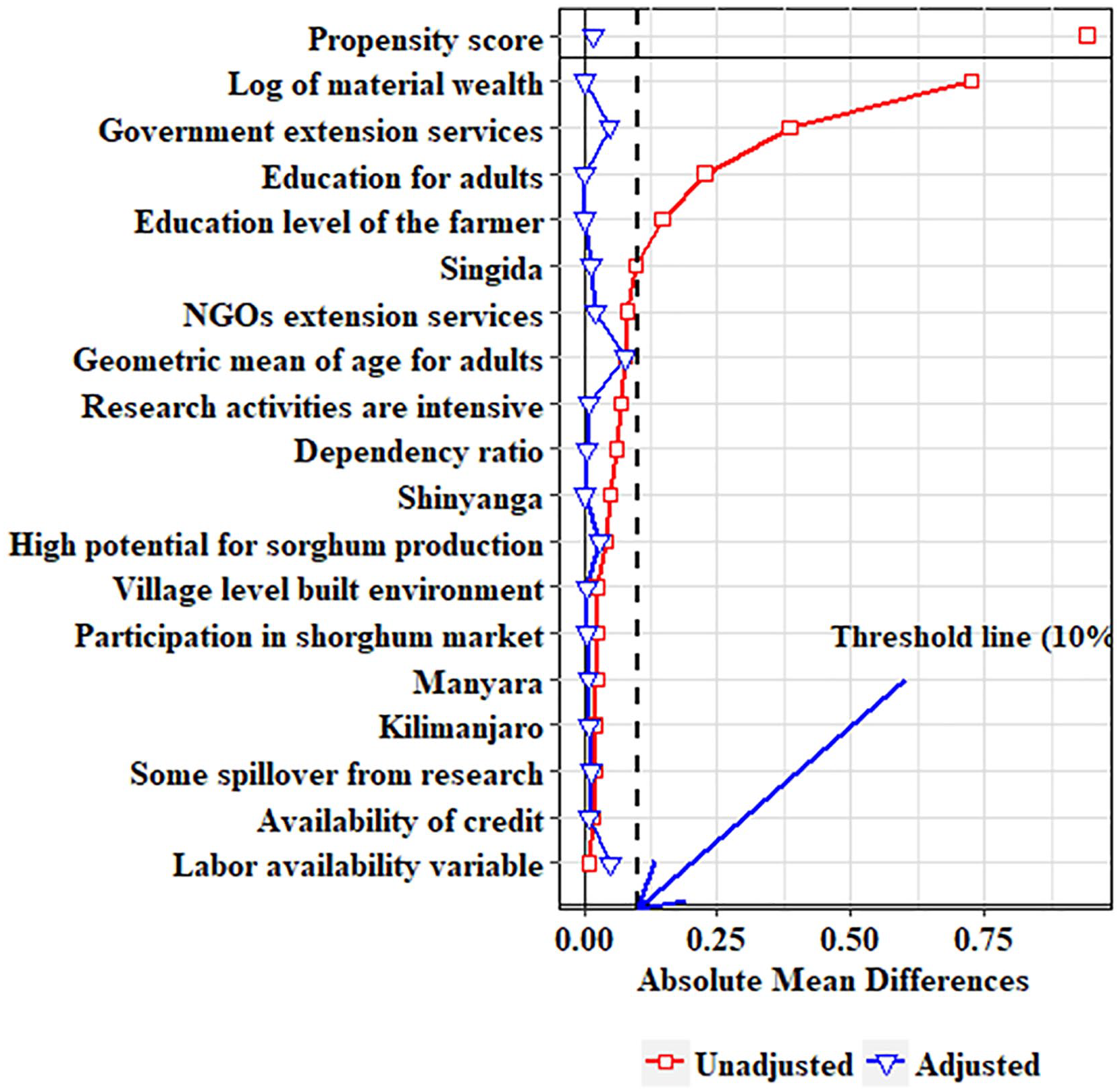
Distribution of absolute mean/proportion difference before and after matching.

Combining the results in Figures 1 and 2 implies that, after weighting, the empirical distributions of adopters’ and nonadopters’ covariates were statistically identical. The welfare model (i.e., the second expression of Equation 1) was, therefore, statistically valid, and according to Hansen (2008), the estimable three effect measures (i.e., ATT, ATE, and ATC) are unbiased and efficient.

Effect of Adoption on Welfare

During the estimation of the welfare model, we could either exclude or include all observations outside the regional common-support [0.0558, 0.937] based on estimated propensity scores explained above (Stuart et al., 2013). Therefore, we applied DiCiccio and Efron’s (1996) bootstrapping technique and different permutation test statistics to determine whether the adoption status coefficients for the two models were from similar empirical cumulative distribution functions. The graphs in Figure 3 are plots of the observed distributions of bootstrapped adoption status coefficients that estimate ATT using IPW and IPWRA estimators. In Figure 3, WTR_ts denotes the results from the Wilcoxon test statistics, MWW_ts indicates the results from the Mann–Whitney–Wilcoxon test statistics, and KSM_ts presents the results from the Kolmogorov–Smirnov test statistics. For all three tests, the ps in Figure 3 denote probability levels (α = .05). The conclusion is that the results from the two models follow a symmetric distribution around zero or from the same population with similar mean and variance. Supplemental Appendix 4 presents similar permutation test statistics results for bootstrapped ATE and ATC from the two models. As explained in Stuart and Ialongo (2010), when estimating effect using IPW and when adopter and nonadopter groups have similar covariate distributions, the results from matched and full samples should be identical due to reduced bias.

Figure 3.

Bootstrapped ATT results from Wilcoxon, Mann–Whitney–Wilcoxon, and Kolmogorov–Smirnov tests.

Because the results of the two models in Figure 3 are almost similar, Table 2 presents the estimated effect of ISVs on HDDS and WDDS using the full sample for both IPW and IPWRA. The columns in Table 2 show estimated ATT (treated), ATE (average), and ATC (control). For each estimator, the values in the first part of the table are weighted regression coefficients. The numbers in brackets are associated intervals at a 95% confidence level. The second part shows the results when testing for model fit. The RS-LRTS represents Rao-Scott likelihood ratio χ². Test statistics and AIC and BIC denote, respectively, Akaike information criteria and Bayesian information criteria discussed in Burnham and Anderson (2004) and Lumley and Scott (2014, 2015). We compare the full model (model with all covariates) and the null model (model with intercept only). The model with small values of RS-LRTS or AIC or BIC is preferred. All three test statistics reject the null hypothesis that all coefficients associated with covariates in Equation 1 are zero and conclude that the full models perform better than the null models. The full results from the IPWRA are provided in supplemental Appendix 5.

Table 2.

Results on the Impact of Adopting ISVs on Dietary Diversity Scores.

Variable	Household dietary diversity			Women dietary diversity
Variable	Treated	Average	Control	Treated	Average	Control
Inverse probability treatment weighting
Intercept	4.48	4.31	4.23	1.77	1.76	1.69
Intercept	[4.17, 4.79]	[4.26, 4.77]	[4.29, 4.77]	[1.60, 1.94]	[1.61, 1.90]	[1.56, 1.82]
Adoption status	0.88	0.75	0.62	0.61	0.56	0.55
Adoption status	[0.52, 1.24]	[0.41, 0.08]	[0.25, 0.99]	[0.41, 0.82]	[0.37, 0.74]	[0.35, 0.75]
RS-LRTS	17.00	17.60	24.60	11.80	11.80	11.33
AIC	5.30	7.40	17.10	7.70	4.10	6.26
BIC	5.80	6.40	3.20	4.90	4.80	6.73
Num. obs.	822	822	822	822	822	822
Inverse probability treatment weighting with regression adjustment
Intercept	4.38	4.37	4.32	1.75	1.61	1.58
Intercept	[0.91, 7.73]	[0.08, 5.27]	[1.09, 3.73]	[0.49, 3.18]	[0.34, 1.36]	[0.27, 3.83]
Adopt status	0.85	0.76	0.58	0.57	0.55	0.52
Adopt status	[0.49, 1.16]	[0.46, 1.07]	[0.27, 0.89]	[0.38, 0.76]	[0.38, 0.73]	[0.35, 0.69]
RS-LRTS	22.10	12.80	8.70	24.00	23.13	26.20
AIC	9.10	11.90	5.60	118.00	111.00	112.00
BIC	9.40	11.30	9.50	114.00	116.00	97.00
Num. obs.	822	822	822	822	822	822

Note. ISVs = new sorghum varieties; AIC = Akaike information criteria; BIC = Bayesian information criteria; RS-LRTS = Rao-Scott likelihood ratio χ².

The intercept coefficient in Table 2 is the expected weighted mean scores adjusted for self-selection and confounding effects. In that case, some observations contribute more weight than others. As we are using stabilized weights, the outliers contribute minimum influence in calculating the weighted mean scores. As shown in Table 2, both weighted HDDS and WDDS were higher among adopters as expected. The adopters’ (treated) weighted HDDS from IPW and IPWRA estimators was, respectively, 4.48 and 4.38. Analogous values for weighted WDDS were, respectively, 1.77 and 1.75. For nonadopters (control), the weighted HDDS and WDDS were 4.23 and 4.32 and 1.69 and 1.58, respectively. For the sample (average), the weighted average scores for both HDDS and WDDS were, respectively, 4.31 and 4.37 and 1.76 and 1.61. These results imply that after accounting for self-selection and confounding effects, the three dietary diversity estimands are below the cutoff points of diversity and micronutrient and macronutrient adequacy. The estimated weighted dietary diversity scores are comparable to results from other studies such as Mbwana et al. (2016), Kinabo et al. (2016), Ochieng et al. (2017), Ntwenya et al. (2017), and Huang et al. (2018) that focus on estimating the sample HDDS and WDDS.

Note that the intervals from the IPWRA estimator in Table 2 are wider and comparatively tighter than the interval from the IPW estimator. The expected weighted mean score for both HDDS and WDDS among nonadopters and the sample follows a similar distribution pattern where intervals from the IPWRA estimator have a wider range when compared with intervals from the IPW estimator. Statistically, while the IPW estimator produces precise results, IPWRA that adjusts for nonrandomness produces more accurate results (Abadie & Imbens, 2006).

Table 2 also presents the estimated ATT, ATE, and ATC represented as coefficients of adoption status variable from IPW and IPWRA estimators. The estimated coefficients are statistically significant at more than .05 probability level, suggesting that the adoption of ISVs has a positive effect on both HDDS and WDDS. On average, the HDDS among adopters (ATT) was, respectively, higher by about 0.88 (using IPW estimators) and 0.85 (using IPWRA) scores when compared with nonadopters with similar characteristics. For ATE and ATC, the results are, respectively, 0.75 and 0.76 and 0.62 and 0.58. Analogous values on WDDS are 0.61 for ATT, 0.56 for ATE, and 0.55 for ATC from the IPW estimator and 0.57 for ATT, 0.55 for ATE, and 0.52 for ATC from the IPWRA estimator. As these scores are determined using unobserved potential outcomes approach, the ATE values are average of the differences between the scores when each sample household adopts ISVs, and the ATC is an average gain if nonadopters take up ISVs. For example, if nonadopters had taken ISVs, the average scores could have increased by about 0.60 points. Notice that the estimated ATE was the averages of ATT and ATC as expected.

The reported marginal changes in Table 2 for both HDDS and WDDS from nonadoption to adoption (estimated effect) may seem small (about 1 point). However, due to limited access to broader food items among sample households, a minor change has a meaningful result. Although postharvest storage innovations had a positive and significant effect on HDDS, due to a low level of dietary diversity, Tesfaye and Tirivayi (2018) estimated ATT and ATC to be about, respectively, 0.25 and 2.01 in Ethiopia. Results from Passarelli et al.’s (2018) study show that access to improved irrigation system leads to increased HDDS in both Ethiopia and Tanzania by about 1 point. These results differ from Smale et al.’s (2018) study, which suggests that the adoption of ISVs did not spiral into dietary diversity adequacy in Mali. The discrepancy is due to differences in yields and intensity of adoption that are higher in Tanzania compared with Mali.

To determine whether farmers at the bottom of the social-economic pyramid benefit from adopting ISVs, Figure 4 presents comparative analysis results (between adopters and nonadopter). The focus is on the variability relative to the wealth of farmers, farmer’s education, the gender of the household head, and the marital status of the household head. For the wealth variable, the comparison included the lower quartile of the wealth distribution. For education, the contrast was between farmers with less than 7 years of education (primary education). The comparison is also between female farmers and unmarried female farmers and widows. The boxplots in Figure 4 (first part left panel) show the HDDS distribution, and the right panel shows the WDDS distribution estimated using IPW and IPWRA estimators through bootstrapping. Even the poorest adopters (low quartile) had higher total wealth compared with nonadopters. Total wealth averaged to US$2,550 per household and ranged from US$1,800 to US$3,850 for adopters and averaged to US$1,000 and ranged from US$400 to US$1,850 for nonadopters. Regarding the HDDS, the distribution ranged from 1.56 to 5.9, with a median of 5 for adopters. Similar values are 0.5 to 4.9, with a median of 4.5 for nonadopters who were equally poor. The weighted score for the middle 50% of adopters within the first quartile ranged from 4.7 to 5.2 and ranged from 3.8 to 4.1 for nonadopters. As for WDDS (Figure 4, the first part of the right panel), it ranged from 0.4 to 2.4 with a median of 2.2 for adopters and from 0 to 1.9 with a median of 1.6 for nonadopters. Similarly, the WDDS for the middle 50% of adopters of the first quartile of wealth ranged from 2.1 to 2.25 and ranged from 1.4 to 1.7 for nonadopters. Although in both cases the HDDS and WDDS are skewed to the right, poor adopters performed better in all five number categories compared with nonadopters.

Figure 4.

Distribution of ATE for poor farmers and farmers with low education.

The results presented in the second part of Figure 4 show that even farmers with low education benefit from the adoption of ISVs. For HDDS (Figure 4, second part left panel), the weighted mean for adopters (head of household has less than 7 years of education) was 3.5. The median and maximum weighted means were, respectively, 5.2 and 5.9. For nonadopters (with low literacy), the minimum and the median were, respectively, 2.5 and 4.3, and the maximum was 5.0. Regarding the value of WDDS (Figure 4, second part right panel), the value was higher among adopters in which the head of the household has less than 7 years of education compared with nonadopters with a similar level of education. Due to biases that exist within the extension system that favor connected farmers (Awotide et al., 2016), educated farmers tend to have more access to extension services. Suvedi et al. (2017) also contend that farmer’s education influences extension participation and, therefore, training, advice, and information received, especially in a developing country such as Tanzania. Results from this study also show that even impoverished farmers and farmers with low education accrue higher benefits from the adoption of ISVs compared with nonadopters, which emphasizes the importance of inclusive and targeted agricultural education and extension systems.

Figure 5 presents comparative analysis results for female farmers (first panel) and single farmers (second panel) for both adopters and nonadopters. For female farmers, the minimum and maximum scores of the HDDS were, respectively, 4.4, and 6.2 with a median of 5.2 among adopters, and the minimum and maximum scores were, respectively, 3.2 and 5.5 with a median of 4.3 for nonadopters. The minimum, maximum, and median scores for the WDDS among adopters (female farmers) were, respectively, 1.4, 2.0, and 1.7, and similar values among nonadopters were, respectively, 1.1, 1.8, and 1.4. The adopters’ median was 17.65% higher compared with the nonadopters’ median. The comparison of unmarried female farmers also produced comparable results where both HDDS and WDDS were higher among adopters compared with nonadopters, as illustrated in the second panel of Figure 5. For unmarried adopters, the HDDS varied from 4.5 to 6.3, and the median was 5.5. For unmarried nonadopters, the HDDS varied from 3.4 to 5.6, and the median was 4.5. The WDDS for unmarried adopters ranged from 1.5 to 2.1, with a median of 1.8, and WDDS ranged from 1.2 to 1.9, with a median of 1.5 for unmarried nonadopters. Female farmers and unmarried female farmers stand to benefit if they adopt ISVs.

Figure 5.

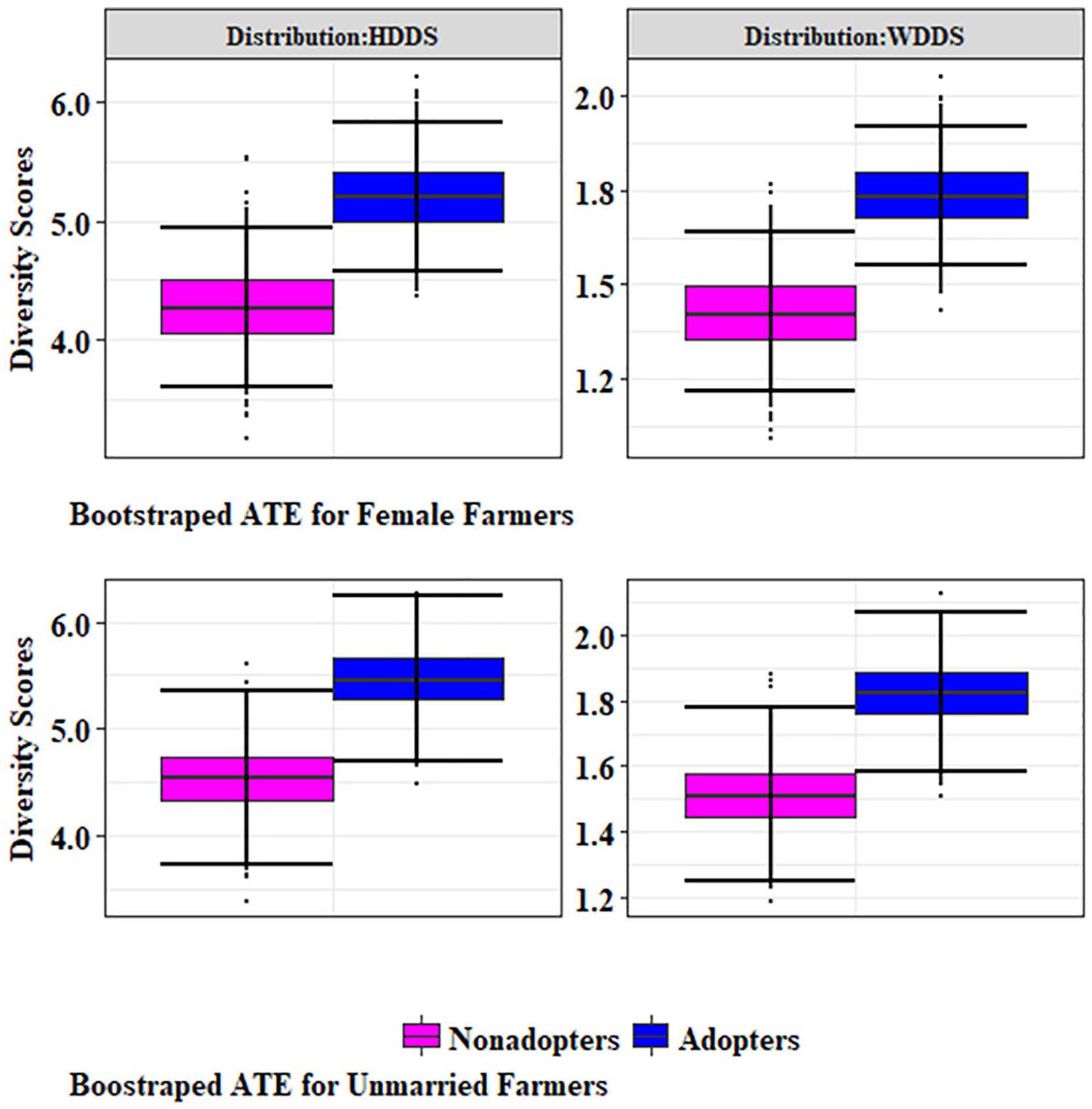
Distribution of ATE for female farmers and unmarried female.

Note that in both Figures 4 and 5, there is no overlap between the boxplots of HDDS and WDDS for adopter and nonadopter groups, which show that the values are statistically higher among adopters. The overall visible spread was over 50%, meaning that the scores for adopters were statistically significantly higher than the scores for nonadopters. Kassie et al. (2011) and Amare et al. (2012) also report improved general welfare among adopters of improved seeds. As improved seeds can increase the productive efficiency of all available resources, ISVs have the potential for both increasing access to diverse food groups and income. Evidence from this study suggests that even those farmers who often appear at the bottom of the socioeconomic pyramid stand to gain from adopting ISVs in Tanzania.

Conclusion

The goal of this study was to explain the complex linkage between improved seed adoption on household and women dietary diversity scores in Tanzania. The study adopts concepts of observational studies explained by Evenson and Gollin (2003) when estimating the effect of adopting agricultural technologies. Observational studies are crucial when randomized controlled trials are infeasible or impractical. Potential for self-selection bias and the presence of cofounder variables that distort the observed relationship between the incidence of adoption and welfare of farmers are the main limitations of observational studies. Controlling for both effects is, therefore, critical in justifying whether the effect of adoption is real or due to chance. The IPW and IPWRA that account for both effects were adapted when estimating the effect of improving sorghum varieties in Tanzania. The household and women dietary diversity scores (i.e., WDDS and HDDS) were indicators of farmers’ general welfare. The HDDS is a qualitative measure of access to varied food groups at the household level, and the WDDS is a measure of micronutrient and macronutrient adequacy (quality) among children and women of reproductive age.

The main results show that the Kilimanjaro Region had the highest scores for both indicators, with the lowest scores recorded in the Shinyanga Region. The marginal effects of adoption were statistically significantly higher among adopters at the 5% probability level. The adoption of ISVs increased HDDS and WDDS by 1 point or food group in the sample. The small but statistically significant marginal changes reflect the low level of access to broader food items in Tanzania. A minor change to increase access will have a significant effective result. Comparative analyses show that even households at the bottom of social-economic pyramids such as female farmers benefited from adoption.

The goals of most agricultural programs include enhancing the welfare of diverse groups of farmers. As proven in this study, the adoption of improved sorghum seeds could increase access to various food groups. Notably, the results from weighting with regression adjustment attest that the existence of institutional support systems is vital in terms of enhancing the welfare of farmers. Advisory services and other extension activities help farmers access these technologies and assess technology costs, risk profiles, and potential economic profitability.

Moreover, research and agricultural extension are the most common model to transmit information to farmers. To scale up and sustain the effect of adoption, a robust pedagogical linkage among research–extension–policy stakeholders is essential in promoting farmer-tailored, easily accessible, and modern agricultural innovations. Training to incentivize extension agents and engagement of policymakers at the community level, such as during farmers’ training and field days, are vital in maintaining the linkage, sustaining, and advocating policies that support farmers’ access to improved seeds and other improved agricultural practices. There is also a need to focus on female and poor farmers to promote universal access to dietary diversity. In general, small-scale agriculture supported by a sustainable and improved crop system will expand the availability and consumption of various food items, which in turn will improve nutritional status and promote positive health outcomes. Poor health outcomes are deeply interrelated with lower agricultural productivity and mutually reinforce each other. There is a genuine appeal to address these problems jointly. The question is, how do we begin to find these linked outcomes? Accordingly, conducting more studies should answer this question.

Supplemental Material

sj-pdf-1-sgo-10.1177_2158244020979992 – Supplemental material for Impact of Adopting Improved Seeds on Access to Broader Food Groups Among Small-Scale Sorghum Producers in Tanzania

Supplemental material, sj-pdf-1-sgo-10.1177_2158244020979992 for Impact of Adopting Improved Seeds on Access to Broader Food Groups Among Small-Scale Sorghum Producers in Tanzania by Aloyce R. Kaliba, Anne G. Gongwe, Kizito Mazvimavi and Ashagre Yigletu in SAGE Open

Footnotes

Declaration of Conflicting Interests

The author(s) declared no potential conflicts of interest with respect to the research, authorship, and/or publication of this article.

Funding

The author(s) disclosed receipt of the following financial support for the research, authorship, and/or publication of this article: The International Crop Research Institute for Semi-Arid Tropics (ICRISAT) in Nairobi, Kenya, funded this study under the Monitoring, Evaluation, Impact, and policy East Africa Program. However, the view expressed in this paper are those of the authors and do not necessarily represent ICRISAT’s view.

ORCID iD

Aloyce R. Kaliba

Supplemental Material

Supplemental material for this article is available online.

References

Abadie

Imbens

G. W.

(2006). Large sample properties of matching estimators for average treatment effects. Econometrica, 74(1), 235–267.

Abebe

Bekele

(2015). Analysis of adoption spell of improved common bean varieties in the central rift valley of Ethiopia: A duration model approach. Journal of Development and Agricultural Economics, 4(3), 37–43.

Ainembabazi

J. H.

Mugisha

(2014). The role of farming experience on the adoption of agricultural technologies: Evidence from smallholder farmers in Uganda. The Journal of Development Studies, 50(5), 666–679.

Amare

Asfaw

Shiferaw

(2012). Welfare effects of maize-pigeon pea intensification in Tanzania. Agricultural Economics, 43(1), 27–43.

Angrist

J. D.

Pischke

J.-S.

(2009). Mostly harmless econometrics: An empiricist’s companion. Princeton University Press.

Arimond

Ruel

M. T.

(2004). Dietary diversity is associated with child nutritional status: Evidence from 11 demographic and health surveys. The Journal of Nutrition, 134(10), 2579–2585.

Asfaw

Shiferaw

Simtowe

Lipper

(2012). Effect of modern agricultural technologies on smallholder welfare: Evidence from Tanzania and Ethiopia. Food Policy, 37(3), 283–295.

Austin

P. C.

(2009). Balance diagnostics for comparing the distribution of baseline covariates between treatment groups in propensity-score matched samples. Statistics in Medicine, 28(25), 3083–3107.

Austin

P. C.

(2011). An introduction to propensity-score methods for reducing the effects of confounding in observational studies. Multivariate Behavioral Research, 46, 399–424.

10.

Austin

P. C.

Grootendorst

Normand

S. L.

Anderson

G. M.

(2007). Conditioning on the propensity score can result in biased estimation of common measures of treatment effect: A Monte Carlo study. Statistics in Medicine, 26(4), 754–768.

11.

Awel

Y.M.

Azomahou

T. T.

(2014). Productivity and welfare effects of weather index insurance: Quasi-experimental evidence. World Bank.

12.

Awotide

B. A.

Karimov

A. A.

Diagne

(2016). Agricultural technology adoption, commercialization, and smallholder rice farmers’ welfare in rural Nigeria. Agricultural and Food Economics, 4, Article 3. https://doi.org/10.1186/s40100-016-0047-8

13.

Bang

Robins

J. M.

(2005). Doubly robust estimation in missing data and causal inference models. Biometrics, 61(4), 962–973.

14.

Becquey

Martin-Prevel

Traissac

Bernard Dembélé

Bambara

Delpeuch

(2010). The household food insecurity access scale and an index-member dietary diversity score contribute valid and complementary information on household food insecurity in an urban West-African setting. Journal of Nutrition, 140(12), 2233–2240.

15.

Bogetoft

Otto

(2018). Benchmarking: Benchmark and frontier analysis using DEA and SFA (R Package Version 0.27). https://CRAN.R-project.org/package=Benchmarking

16.

Burnham

K. P.

Anderson

D. R.

(2004). Multimodal inference: Understanding AIC and BIC in model selection. Sociological Methods and Research, 33(2), 261–304.

17.

Caliendo

Kopeinig

(2008). Some practical guidance for the implementation of propensity score matching. Journal of Economics Survey, 22(1), 31–72.

18.

Cattaneo

M. D.

(2000). Efficient semiparametric estimation of multi-valued treatment effects under ignorability. Journal of Econometrics, 155, 138–154.

19.

Chakona

Shackleton

(2017). Minimum dietary diversity scores for women indicate micronutrient adequacy and food insecurity status in South African Towns. Nutrients, 9(8), 812.

20.

Charnes

Cooper

W. W.

Rhodes

(1978). Measuring the efficiency of decision-making units. European Journal of Operational Research, 2, 429–444.

21.

Chen

Ravallion

(2007). Absolute poverty measures for the developing world, 1981-2004 (Policy Research Working Paper No. 4211). World Bank. https://openknowledge.worldbank.org/handle/10986/7060

22.

Dalton

T. J.

Zereyesus

Y. A.

(2013). Economic effect assessment of sorghum, millet, and other grains CRSP: Sorghum and millet germplasm development research (Paper 20). INTSORMIL Scientific Publications.

23.

Dehejia

Wahba

(1999). Causal effects in non-experimental studies: Re-evaluating the evaluation of training programs. Journal of the American Statistical Association, 94(448), 1053–1062.

24.

Despotis

D. K.

(2005). A reassessment of the human development index via data envelopment analysis. Journal of the Operational Research Society, 56, 969–980.

25.

DiCiccio

T. J.

Efron

(1996). Bootstrap confidence intervals (with discussion). Statistical Science, 11, 189–228.

26.

Doss

Mwangi

Verkuijl

de Groote

(2003). Adoption of maize and wheat technologies in Eastern Africa: A synthesis of the findings from 22 case studies (CIMMYT Economics Working Paper 03-06). Centro Internacional de Mejoramiento de Maíz y Trigo.

27.

Ecker

(2018). Agricultural transformation and food and nutrition security in Ghana: Does farm production diversity (still) matter for household dietary diversity? Food Policy, 79, 271–282.

28.

Ellis

(1998). Household strategies and rural livelihood diversification. The Journal of Development Studies, 35(1), 1–38.

29.

Etikan

Bala

(2017). Sampling and sampling methods. Biometrics and Biostatistics International Journal, 5(6), 215–217. https://doi.org/10.15406/bbij.2017.05.00149

30.

European Food Safety Authority. (2009). General principles for the collection of national food consumption data in the view of a pan-European dietary survey. EFSA Journal, 7(12), 1435. https://doi.org/10.2903/j.efsa.2009.1435

31.

Evenson

R. E.

Gollin

(2003). Assessing the effect of the green revolution, 1960 to 2000. Science, 300(5620), 758–762.

32.

Faber

Weinhold

F. A. M

Laurie

S. M.

(2017). Dietary diversity and vegetable and fruit consumption of households in a resource-poor peri-urban South Africa community differ by food security status. Ecology of Food and Nutrition, 56, 62–80. https://doi.org/10.1080/03670244.2016.1261024

33.

Farrell

M. J.

(1957). The measurement of productive efficiency. Journal of the Royal Statistical Society, 120(3), 253–290.

34.

Food and Agriculture Organization of the United Nations. (2014). The Minimum Dietary Diversity for Women (MDD-W) indicator. http://www.fao.org/nutrition/assessment/tools/minimum-dietary-diversity-women/en/

35.

Funk

M. J.

Westreich

Wiesen

Stürmer

T. M.

Alan Brookhart

M. A.

Davidian

(2011). Doubly robust estimation of causal effects. American Journal of Epidemiology, 173(7), 761–767.

36.

Gernand

A. D.

Schulze

K. J.

Stewart

C. P.

West

K. P.

Jr. Christian

(2016). Micronutrient deficiencies in pregnancy worldwide: Health effects and prevention. Nature Reviews Endocrinology, 12(5), 274–289.

37.

Gina

L. K.

Maria Regina Pedro

M. R.

Seghieri

Nantel

Brouwer

(2007). Dietary diversity score is a useful indicator of micronutrient intake in non-breast-feeding Filipino children. The Journal of Nutrition, 137, 472–477.

38.

Glynn

A.N.

Quinn

K. M.

(2010). An introduction to the augmented inverse propensity weighted estimator. Political Analysis, 18, 36–56.

39.

Greifer

(2019). cobalt: Covariate balance tables and plots (R Package Version 2.2.0). https://CRAN.R-project.org/package=cobalt

40.

Guo

Fraser

M. W.

(2010). Propensity score analysis: Statistical methods and applications. Psychometrika, 75(4), 775–777.

41.

Hansen

B. B.

(2008). The prognostic analog of the propensity score. Biometrika, 95, 481–488.

42.

Hatloy

Hallund

Diarra

Oshaug

(2000). Food variety, socioeconomic status and nutritional status in urban and rural areas in Koutiala (Mali). Public Health Nutrition, 3(1), 57–65.

43.

Heckman

Vytlacil

(2007). Econometric evaluation of social programs, part I: Causal models, structural models, and econometric policy evaluation. In Heckman

J. J.

Leamer

E. E.

(Eds.), Handbook of econometrics, (1st ed., Volume 6B, Chapter 70, pp. 4779–4874). Elsevier.

44.

Holden

Shiferaw

Pender

(2001). Market imperfections and land productivity in the Ethiopian Highlands. Journal of Agricultural Economics, 52(3), 53–70.

45.

Huang

Sudfeld

Ismail

Vuai

Ntwenya

Mwanyika-Sando

Fawzi

(2018). Maternal dietary diversity and growth of children under 24 months of age in rural Dodoma, Tanzania. Food Nutrition Bulletin, 39(2), 219–230.

46.

Imai

van Dyk

D. A.

(2004). Causal Inference with general treatment regimens: Generalizing the propensity score. Journal of the American Statistical Association, 99, 854–866.

47.

Jones

A. D.

(2017). On-farm crop species richness is associated with household diet diversity and quality in subsistence- and market-oriented farming households in Malawi. Journal of Nutrition, 147, 86–96.

48.

Jones

A. D.

Ngure

F. M.

Pelto

Young

S. L.

(2013). What are we assessing when we measure food security? A compendium and review of current metrics. Advanced Nutrition, 4(5), 481–505.

49.

Kabunga

N. S.

Dubois

Qaim

(2014). Effect of tissue culture banana technology on farm household income and food security in Kenya. Food Policy, 45, 25–34.

50.

Kaliba

A. R.

Mazvimavi

Ghebreyesus

G. S.

(2017). Economic profitability and risk analyses of improved sorghum varieties in Tanzania. Journal of Development and Agricultural Economics, 9(9), 250–268.

51.

Kaliba

A. R.

Mazvimavi

Gregory

T. L.

Mgonja

F. M.

Mgonja

(2018). Factors affecting adoption of improved sorghum varieties in Tanzania under information and capital constraints. Agricultural Economics, 6(18). https://doi.org/10.1186/s40100-018-0114-4.

52.

Kang

J. D. Y.

Schafer

J. L.

(2007). Demystifying double robustness: A comparison of alternative strategies for estimating a population means from incomplete data. Statistical Science, 22, 523–539.

53.

Kanyeka

Kamala

Kasuga

(2007). Improved agricultural research technologies that are recommended for Tanzania. The Department of Research & Training, Ministry of Agriculture Food Security and Cooperatives.

54.

Kassie

Shiferaw

Muricho

(2011). Agricultural technology, crop income, and poverty alleviation in Uganda. World Development, 39(10), 1784–1795.

55.

Kebede

W. M.

Tadesse

(2015). Factors affecting the adoption of malt-barley technology: Evidence from North Gondar Ethiopia. Journal of Food Security, 3(3), 75–81.

56.

Keding

G. B.

Msuya

J. M.

Maass

B. L.

Krawinkel

M. B.

(2012). Relating dietary diversity and food variety scores to vegetable production and socio-economic status of women in rural Tanzania. Food Security, 4(1), 129–140.

57.

Kendall

Olson

C. M.

Frongillo

E. A.

(1996). Relationship of hunger and food insecurity to food availability and consumption. Journal of American Diet Association, 96, 1019–1024.

58.

Kennedy

G. L.

Ballard

Dop

(2013). Guidelines for measuring household and individual dietary diversity. Nutrition and Consumer Protection Division, Food and Agriculture Organization of the United Nations. http://www.fao.org/3/a-i1983e.pdf

59.

Kennedy

G. L.

Pedro

M. R.

Seghieri

Nantel

Brouwer

(2007). Dietary diversity score is a useful indicator of micronutrient intake in non-breast-feeding Filipino children. The Journal of Nutrition, 137(2), 472–477.

60.

Khonje

Manda

Alene

Kassie

(2015). Analysis of adoption and effects of improved maize varieties in eastern Zambia. World Development, 66, 695–706.

61.

Kilimo. (2008). Tanzania variety list. Ministry of Agriculture, Livestock, and Fisheries Development. https://www.kilimo.go.tz/index.php/en/resources/view/tanzania-variety-list-updated-to-2008

62.

Kinabo

Mamiro

Dawkins

Bundala

Mwanri

Majili

Jumbe

Kulwa

Mamiro

Amuri

Ngowi

Msuya

(2016). Food intake and dietary diversity of farming households in Morogoro region, Tanzania. African Journal of Food, Agriculture, Nutrition and Development, 16(4), 11295–11309.

63.

Koppmair

Kassie

Qaim

(2017). Farm production, market access, and dietary diversity in Malawi. Public Health Nutrition, 20, 325–335.

64.

Lee

B. K.

Lessler

Stuart

E. A.

(2011). Weight trimming and propensity score weighting. PLOS ONE, 6(39), e18174. https://doi.org/10.1371/journal.pone.0018174

65.

Linden

(2017). Improving causal inference with a doubly robust estimator that combines propensity score stratification and weighting. Journal of Evaluation in Clinical Practices, 23, 697–702. https://doi.org/10.1111/jep.12714

66.

Luckett

B. G.

DeClerck

F. A. J.

Fanzo

Mundorf

A. R.

Rose

(2015). Application of the nutrition functional diversity indicator to assess food system contributions to dietary diversity and sustainable diets of Malawian households. Public Health Nutrition, 18(13), 2479–2487.

67.

Lumley

(2018). Survey: Analysis of complex survey samples (R Package Version 3.31-2). https://www.R-project.org

68.

Lumley

Scott

A. J.

(2014). Tests for regression models fitted to survey data. Australia and New Zealand Journal of Statistics, 56(1), 1–14.

69.

Lumley

Scott

A. J.

(2015). AIC and BIC for modeling with complex survey data. Journal of Survey Statistical Methods, 3(1), 1–18.

70.

Mahlberg

Obersteiner

(2001). Remeasuring the HDI by data envelopment analysis [IIASA Interim Report IR-01-069]. International Institute for Applied Systems Analysis. http://pure.iiasa.ac.at/6455/

71.

Martin-Prével

Allemand

Wiesmann

Arimond

Ballard

Deitchler

Marie-Claude Dop

M. C.

Kennedy

Lee

W. T. K.

Moursi

(2015). Moving forward. On choosing a standard operational indicator of women’s dietary diversity. Food and Agriculture Organization of the United Nations. http://www.fao.org/3/a-i4942e.pdf

72.

Mason

N. M.

Smale

(2013). Effects of subsidized hybrid seed on indicators of economic well-being among smallholder maize growers in Zambia. Agricultural Economics, 44(6), 659–670.

73.

Mathenge

M. K.

Smale

Olwande

(2014). The effects of hybrid maize seed on the welfare of farming households in Kenya. Food Policy, 44, 262–271.

74.

Mbwana

H. A.

Kinabo

Lambert

Biesalski

H. K.

(2016). Determinants of household dietary practices in rural Tanzania: Implications for nutrition interventions. Cogent Food & Agriculture, 2(1). https://doi.org/10.1080/23311932.2016.1224046

75.

Mgonja

M. A.

Chandra

Gwata

E. T.

Obilana

A. B.

Monyo

E. S.

Rohrbach

D. D.

Chisi

Kudita

Saadan

H. M.

(2005). Improving the efficiencies of national crop breeding programs through region-based approaches: The case of sorghum and pearl millet in Southern Africa. Journal of Food, Agriculture and Environment, 3, 124–129.

76.

Mwangi

Kariuki

(2015). Factors determining the adoption of new agricultural technology by smallholder farmers in developing countries. Journal of Economics and Sustainable Development, 6(5). https://www.iiste.org/Journals/index.php/JEDS/article/view/20710

77.

Nelson

Bingham

S. A.

(1997). Assessment of food consumption and nutrient intake. In Margetts

B. M.

Nelson

(Eds.), Design concepts in nutritional epidemiology (2nd ed., pp. 123–169). Oxford University Press.

78.

Ntwenya

J. E.

Kinabo

Msuya

Mamiro

Njoghomi

Liwei

Huang

(2017). Rich food biodiversity amid low consumption of food items in Kilosa District, Tanzania. Food and Nutrition Bulletin, 38, 501–511. https://doi.org/10.1177/0379572117708647

79.

Ochieng

Afari-Sefa

Lukumay

P. J.

Dubois

(2017). Determinants of dietary diversity and the potential role of men in improving household nutrition in Tanzania. PLOS ONE, 12, e0189022. https://doi.org/10.1371/journal.pone.0189022

80.

Operations Evaluation Department. (2011). Improving food security: A systematic review of the effect of interventions in agricultural production, value chains, market regulation, and land security (IOB Study No. 363). Ministry of Foreign Affairs. https://www.oecd.org/derec/49558328.pdf

81.

Passarelli

Mekonnen

Bryan

Ringler

(2018). Evaluating the pathways from small-scale irrigation to dietary diversity: Evidence from Ethiopia and Tanzania. Food Security, 10(2), 981–997.

82.

Population Council. (1996). The Rome declaration on world food security. Population and Development Review, 22(4), 807–809.

83.

Ravallion

Chen

(1997). What can new survey data tell us about recent changes in distribution and poverty? The World Bank Review, 11(2), 357–382.

84.

R Core Team. (2019). R: A language and environment for statistical computing. R Foundation for Statistical Computing. https://www.R-project.org/

85.

Robins

J. M.

Sued

Lei-Gomez

Rotnitzky

(2007). Comment: Performance of double- robust estimators when inverse probability weights are highly variable. Statistical Science, 22(4), 544–559.

86.

Rosenbaum

P. R.

Rubin

D. B.

(1983). The central roles of the propensity score in observational studies for causal effects. Biometrika, 70, 41–55.

87.

Rosenbaum

P. R.

Rubin

D. B.

(1985). Constructing a control group using multivariate matched sampling methods that incorporate the propensity score. American Statistician, 36, 65–78.

88.

Rubin

D. B.

(1974). Estimating causal effects of treatments in randomized and non-randomized studies. Journal of Educational Psychology, 66, 688–701.

89.

Savy

Martin-Prével

Sawadogo

Kameli

Delpeuch

(2005). Use of variety/diversity scores for diet quality measurement: Relation with nutritional status of women in a rural area in Burkina Faso. European Journal of Clinical Nutrition, 59, 703–716.

90.

Shadish

W. R.

Clark

M. H.

Steiner

P. M.

(2008). Can nonrandomized experiments yield accurate answers? A randomized experiment comparing random to a nonrandom assignment. Journal of the American Statistical Association, 103, 1334–1343.

91.

Sharpe

Andrews

(2010). An assessment of weighting methodologies for composite indicators: The case of the index of economic well-being (CSLS Research Report No. 10). Centre for the Study of Living Standards.

92.

Shiferaw

Kassie

Jaleta

Yirga

(2014). Adoption of improved wheat varieties and effects on household food security in Ethiopia. Food Policy, 44, 272–284.

93.

Sibhatu

K. T.

Qaim

(2018). Review: A meta-analysis of the association between production diversity, diets, and nutrition in smallholder farm households. Food Policy, 77, 1–18.

94.

Sisay

Haji

Goshu

Edriss

A.-K.

(2015). Technical, allocative, and economic efficiency among smallholder maize farmers in Southwestern Ethiopia: Parametric approach. Journal of Development and Agricultural Economics, 7(8), 282–291.

95.

Skelly

A. C.

Dettori

J. R.

Brodt

E. D.

(2012). Assessing bias: The importance of considering confounding. Evidence-Based Spine-Care Journal, 3(1), 9–12.

96.

Smale

Assima

Kergna

Thériault

Weltzien

(2018). Farm family effects of adopting improved and hybrid sorghum seed in the Sudan Savanna of West Africa. Food Policy, 74, 162–171.

97.

Smale

Mason

N. M.

(2014). Hybrid seed and the economic well-being of smallholder maize farmers in Zambia. Journal of Development Studies, 50(5), 680–695.

98.

Smale

Moursi

Birol

(2015). How does adopting hybrid maize affect dietary diversity on family farms? Micro-evidence from Zambia? Food Policy, 52, 44–53.

99.

Somarriba

Pena

(2009). Synthetic indicators of quality of life in Europe. Social Indicator Research, 94, 115–133.

100.

Stuart

E. A.

(2010). Matching methods for causal inference: A review and a look forward. Statistical Science, 25(1), 1–21.

101.

Stuart

E. A.

Ialongo

N. S.

(2010). Matching methods for selection of subjects for follow-up. Multivariate Behavior Research, 45(4), 746–765.

102.

Stuart

E. A.

Lee

B. K.

Leacy

F. P.

(2013). Prognostic score-based balance measures can be a useful diagnostic for propensity score methods in comparative effectiveness research. Journal of Clinical Epidemiology, 66, S84–S90.e1.

103.

Suvedi

Ghimire

Kaplowitz

(2017). Farmers’ participation in extension programs and technology adoption in rural Nepal: A logistic regression analysis. The Journal of Agricultural Education and Extension, 23(2), 1–21.

104.

Swindale

Bilinsky

(2006). Household Dietary Diversity Score (HDDS) for measurement of household food access: Indicator guide (Version 2, FHI 360). https://www.fantaproject.org/sites/default/files/resources/HDDS_v2_Sep06_0.pdf

105.

Tesfaye

Tirivayi

(2018). The effects of postharvest storage innovations on food security and welfare in Ethiopia. Food Policy, 75, 52–67.

106.

Thompson

F. E.

Byers

(1994). Dietary assessment resource manual. Journal of Nutrition, 124(11 Suppl), 2245S–2317S.

107.

Thomson

Gelson

Kuntashula

(2014). Adoption of improved maize seed varieties in Southern Zambia. Asian Journal of Agricultural Sciences, 6(1), 33–39.

108.

Uysal

S. D.

(2015). Doubly robust estimation of causal effects with multivalued treatments: An application to the returns to schooling. Journal of Applied Econometrics, 30(5), 763–786.

109.

Webb

Coates

Frongillo

E. A.

Rogers

B. L.

Swindale

Bilinsky

(2006). Measuring household food insecurity: Why it’s so important and yet so difficult to do? Journal of Nutrition, 136, 1404–1408.

110.

Wooldridge

J. M.

(2002). Inverse probability weighted m-estimation for sample selection, attrition, and stratification. Portuguese Economic Journal, 1, 117–139.

111.

Wooldridge

(2007). Inverse probability weighted estimation for general missing data problems. Journal of Econometrics, 141(2), 1281–1301.

112.

World Food Program. (2005). Emergency food security assessment handbook. https://www.wfp.org/publications/emergency-food-security-assessment-handbook

113.

Zhao

Tan

Zheng

Zhao

Wang

Zhang

(2017). Dietary diversity scores: An indicator of micronutrient inadequacy instead of obesity for Chinese children. BMC Public Health, 17, Article 440. https://doi.org/10.1186/s12889-017-4381-x

Supplementary Material

Please find the following supplemental material available below.

For Open Access articles published under a Creative Commons License, all supplemental material carries the same license as the article it is associated with.

For non-Open Access articles published, all supplemental material carries a non-exclusive license, and permission requests for re-use of supplemental material or any part of supplemental material shall be sent directly to the copyright owner as specified in the copyright notice associated with the article.

0.00 MB

0.23 MB