Sage Journals: Discover world-class research

Abstract

This study emphasizes the necessity of the Harrod-neutral identification of technological progress for the models of economic growth, which use Cobb–Douglas production function and which are based on stability. Some of the important studies, which reviewed a balanced growth path or a steady state of the Solow model, assumed the nature of technological progress as Hicks-neutral rather than Harrod-neutral. In this work, we have reminded that Harrod-neutral is a better assumption for the nature of technological progress in such studies.

Keywords

Hicks-neutral Harrod-neutral technological progress growth stability

Introduction

Models of economic growth based on long-term equilibrium, which assumed the nature of technological progress as Hicks-neutral cause the following contradiction: For the models of economic growth based on long-term equilibrium, if Hicks-neutral technological change is assumed, the economy can never reach equilibrium; that is, long-term equilibrium cannot be established. The above contradiction can only be resolved if either the level of technology is assumed to be constant over time or the Hicks-neutral assumption of technological progress is replaced with Harrod-neutral assumption.

Many research articles such as Uzawa (1961), Inada (1964), Allen (1967), Inada (1969), and Burmeister and Dobell (1970) have already showed that Harrod-neutral technological progress is compatible with stability. Acikgoz and Mert (2014) further emphasized the importance of this assumption for time-series econometric analysis. This present study aims to emphasize that the nature of technological progress should be assumed rather than Harrod-neutral for mathematical models of economic growth, which are based on stability.

This study is organized as follows. The section “Main Problem” discusses the main problem of the study. In the section “Selected Studies in Literature,” we provide some studies that support our hypothesis. The section “Conclusion” states the concluding remarks.

Main Problem

The main problem is the assumption of the nature of technological progress in models of economic growth based on long-term equilibrium. The nature of the technological progress is usually assumed as Hicks-neutral or Harrod-neutral.

According to Hicks (1963), Hicks-neutral technological progress occurs if the capital–labor ratio does not change, while the ratio of factor prices is constant. According to Harrod (1948), Harrod-neutral technological progress occurs if the capital–output ratio does not change, while the marginal productivity per labor capital stock is constant.

We give an example with regard to Solow (1956).

Solow (1956) gives the following basic equation:

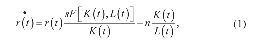
\overset{•}{r (t)} = r (t) \frac{s F [K (t), L (t)]}{K (t)} - n \frac{K (t)}{L (t)},

where $\overset{•}{r (t)}$ is the change in the capital–labor ratio, K(t) is the physical capital stock, L(t) is labor, s is the saving rate, and n is the constant growth rate of labor. At the steady-state conditions, $\overset{•}{r (t)}$ is equal to 0. Then, the following equation can be written:

r (t) \frac{s F [K (t), L (t)]}{K (t)} = n \frac{K (t)}{L (t)} .

As r(t) is the capital–labor ratio and the output $Y (t)$ is $F [K (t), L (t)],$ Equation 2 is rewritten as

\frac{s Y (t)}{L (t)} = n \frac{K (t)}{L (t)} .

Note that the Cobb–Douglas production function with constant returns to scale is as follows:

Y (t) = K {(t)}^{α} L {(t)}^{1 - α},

where α is the elasticity of capital with respect to output.

If the level of technology $A$ is imposed on the production function as Hicks-neutral, then Equation 4 becomes Equation 5:

Y (t) = A K {(t)}^{α} L {(t)}^{1 - α} .

At the steady-state conditions, using Equation 5, Equation 3 is rewritten as Equation 6:

\frac{s A K {(t)}^{α} L {(t)}^{1 - α}}{L (t)} = n \frac{K (t)}{L (t)} .

\frac{K (t)}{L (t)} = {(\frac{s A}{n})}^{\frac{1}{1 - α}} .

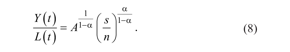
Equation 7 gives the capital–labor ratio at the steady state, when the nature of technological progress is defined as the Hicks-neutral. Thus, Equation 8 is written at the steady state for the output–labor ratio, when the nature of the technological progress is Hicks-neutral.

\frac{Y (t)}{L (t)} = A^{\frac{1}{1 - α}} {(\frac{s}{n})}^{\frac{α}{1 - α}} .

Proposition 1: If it is assumed that the nature of technological progress is Hicks-neutral, then the level of technology should be constant for stability; that is, the level of technology cannot change over time.

Simple Proof of Proposition 1: Assume that, for all positive values of A, which are greater than 1, ceteris paribus, the level of technology rises from A₁ to A₂. Then, according to Equation 8 $A_{2}^{\frac{1}{1 - α}} {(\frac{s}{n})}^{\frac{α}{1 - α}} > A_{1}^{\frac{1}{1 - α}} {(\frac{s}{n})}^{\frac{α}{1 - α}} .$ For simplicity,kindly assume that $s = n$ and $α = .5.$ Then, it is true that ${(\frac{Y (t)}{L (t)})}_{2} = A_{2}^{2} > {(\frac{Y (t)}{L (t)})}_{1} = A_{1}^{2}$ for all positive values ofA, which are greater than 1. If the level of technology rises, for example, 5%, then at the steady state, the output–labor ratio and the capital–labor ratio shouldgrow at the same rate. However, since ${(\frac{Y (t)}{L (t)})}_{2} = A_{2}^{2}$ and ${(\frac{Y (t)}{L (t)})}_{1} = A_{1}^{2},$ the output–labor ratio grows faster thanthe level of technology; that is, steady-state conditions are not established. Better yet, note that Equation 5 is rewritten as $g_{Y} - g_{L} = g_{A} + α (g_{K} - g_{L}),$ where g is the growth rate of the relevant variables. It is obvious that if and only if the growth rate of technology $(g_{A})$ is equal to 0, then the steady-state conditions are established; that is, $g_{Y} - g_{L} = g_{K} - g_{L} = g_{A} = 0 .$

Indeed, Solow (1956) confirms the proposition stated above, by extending his model with the neutral technological change. He uses the following production function:

Y (t) = A (t) F (K, L),

where technology grows at a constant rate $[A (t) = e^{g t}] .$ Importantly, Solow (1956) makes a solution for the long run and shows that the “capital-labor ratio never reach an equilibrium but grows forever” (p. 85). In other words, if the level of technology changes over time, then the economy can never reach the equilibrium.

Selected Studies in the Literature

Some of the selected studies in the literature will be summarized as per our concerns. First, Uzawa (1961) emphasizes that Solow (1956) and Swan (1956) had been discussed for a case in which technical inventions are neutral in Hicks’s sense. However, Uzawa (1961) proves the stability of the growth equilibrium in a neoclassical growth model with neutral inventions in Harrod’s sense. Inada (1964) incorporates neutral technical progress in Harrod’s sense into Solow’s model, which assumes no technical progress. Inada (1964) shows the existence and relative stability of the balanced growth when there is Harrod-neutral technical progress. Inada (1969) similarly emphasizes Harrod-neutrality when defining Arrow type models:

Technical progress is endogenous, embodied and neutral in Harrod’s sense, and is such that labour efficiency is a power function of cumulative gross investment. We call this the Arrow type of technical progress. He assumed a fixed coefficient production function and has shown the existence of a steady growth path. (p. 99)

Mirrlees (1967) demonstrates “a method of calculating optimum policies for one-good models with Harrod-neutral technological change” and “prove the conditions for existence of an optimum policy, and show the general shape of the optimum development of such an economy” (p. 95). He emphasizes that “once the assumption of Harrod-neutral technological change is abandoned, steady growth, in terms of the obvious variables, is impossible” (p. 118). Akerlof and Nordhaus (1967) assumed that a model with “a single-good, neo-classical world with capital-augmenting and Hicks-neutral technological change” (p. 343) based on Solow (1959). Akerlof and Nordhaus showed that a balanced growth with a technological change may be a razor’s edge case. According to them, economists who are interested in long-run growth models might begin to think in terms of models showing unbalanced growth with production functions that are not the Cobb–Douglass type. Burmeister and Dobell (1970) clearly show that “unless technological change is ultimately Harrod-neutral, one-sector models generally cannot approach an equilibrium balanced growth path that is economically meaningful” (p. 79).

Steedman (1985) presents “a number of significant, alternative sufficient conditions under which Hicks neutral technical change is an impossibility (and is not merely empirically implausible)” (p. 746). Moreover, Steedman concludes, “It might not be unreasonable to suggest that those who do assume it . . . are obliged to show explicitly that assumption is compatible with their other assumptions” (p. 758).

According to Barro (1990), “The economy is always at a position of steady-state growth” (p. 106). He uses a production function specified with Hicks-neutral technological progress but where technology is constant over time. Thus, Barro (1990) is a study in which explanations on steady state are compatible with the nature of technological progress. Finally, also Samuelson (1965) and Drandakis and Phelps (1966) prove that under some conditions, the economy will converge to a balanced growth path in which technical progress is Harrod-neutral.

It is important to explain Romer (1990) and Lucas (1988) more closely, to clear our argument.

Romer (1990) writes output (Y) using Equation 10:

Y (H_{A}, L, x) = {(H_{Y} A)}^{α} {(L A)}^{β} K^{1 - α - β} η^{α + β - 1},

where $H_{A}$ is the marginal product of research sector, x is the input used by a firm that produces the final output, $H_{Y}$ is the human capital devoted to the final output, η is the unit of forgone consumption to create one unit of any type of durable.

Thus, by differentiating,

g_{Y} = α g_{H_{Y}} + (α + β) g_{A} + β g_{L} + (1 - α - β) g_{K} + (α + β - 1) g_{η} .

Note that according to Romer (1990), $K = η A \bar{x} .$ Thus, $g_{K} = g_{η} + g_{A} + g_{\bar{x}},$ so, $g_{K} - g_{A} - g_{\bar{x}} = g_{η} .$ Therefore, Equation 11 is written as

g_{Y} = α g_{H_{Y}} + (α + β) g_{A} + β g_{L} + (1 - α - β) g_{K} + (α + β - 1) (g_{K} - g_{A} - g_{\bar{x}}) .

As population and human capital devoted to the final output are constant at Romer (1990) $g_{L} = 0$ and $g_{H_{Y}} = 0,$ we can write Equation 13 as

g_{Y} = (α + β) g_{A} + (1 - α - β) g_{K} + (α + β - 1) (g_{K} - g_{A} - g_{\bar{x}}) .

As along the balanced growth path, $\bar{x}$ is constant (Romer, 1990), $g_{\bar{x}} = 0 .$ Besides, along the balanced growth path, the ratio of K to A should also be constant (Romer, 1990), then $g_{η} = 0 .$

Finally rearranging Equation 13, we can write Equation 14 as follows:

g_{Y} = g_{A} .

Since $g_{K} = g_{η} + g_{A} + g_{\bar{x}},$ so,

g_{K} = g_{A} .

Hence, it is shown that Romer (1990) explains steady state using an approach based on endogenous technological progress. Note that Romer (1990) does not assume technology as the type of technical change augmenting all factors in the same way, that is Hicks-neutral.

However, Lucas (1988) is based on a different approach when explaining neoclassical growth theory. He gives the following equation:

N (t) c (t) + \overset{•}{K (t)} = A (t) K {(t)}^{β} N {(t)}^{1 - β},

where $N (t)$ is labor, $c (t)$ is the per capita consumption, β is the elasticity of capital with respect to output. Then, it is obvious that Lucas (1988) assumes Hicks-neutral technological progress, and moreover, technology grows over time at a rate that equals µ.

The right side of Equation 16 shows output, Q. Then, per capita output growth equals

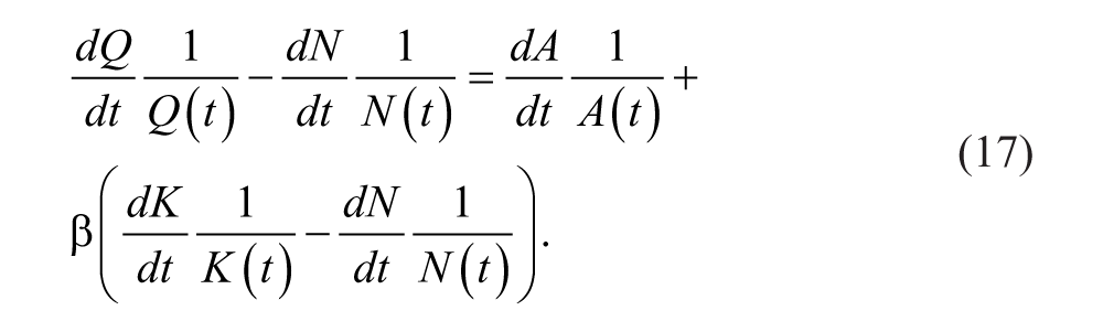
\frac{d Q}{d t} \frac{1}{Q (t)} - \frac{d N}{d t} \frac{1}{N (t)} = \frac{d A}{d t} \frac{1}{A (t)} + β (\frac{d K}{d t} \frac{1}{K (t)} - \frac{d N}{d t} \frac{1}{N (t)}) .

According to Lucas (1988), at a balanced path, per capita capital and per capita consumption grow at a common rate, which is equal to Equation 18:

\frac{d K}{d t} \frac{1}{K (t)} - \frac{d N}{d t} \frac{1}{N (t)} = \frac{μ}{1 - β} .

Thus, according to Lucas (1988), while per capita capital and per capita consumption grow at a common rate, which is equal to $\frac{μ}{1 - β},$ per capita output grows at a rate of $\frac{d A}{d t} \frac{1}{A (t)} + β \frac{μ}{1 - β} .$ Rearranging the equation, per capita output grows at a rate of

\frac{d Q}{d t} \frac{1}{Q (t)} - \frac{d N}{d t} \frac{1}{N (t)} = μ (1 + \frac{β}{1 - β}) = \frac{μ}{1 - β} .

Note that Lucas (1988) says that for the off-steady states, $\frac{μ}{1 - β}$ “need not hold and capital and output growth rates need not to be equal or constant” (p. 15). Hence, according to him, $\frac{μ}{1 - β}$ is used for the steady state.

However, since $\frac{d Q}{d t} \frac{1}{Q (t)} - \frac{d N}{d t} \frac{1}{N (t)} = \frac{d K}{d t} \frac{1}{K (t)} - \frac{d N}{d t} \frac{1}{N (t)} = \frac{μ}{1 - β} \neq μ,$ there is not a steady state due to the fact that the level of technology is also assumed as a variable (it means that it is the level of technology over time), and at the balanced path, all the variables should grow at a common rate. As presented within Proposition 1 in this present study, if the level of technology does not change over time and if it is assumed constant, then $\frac{d Q}{d t} \frac{1}{Q (t)} - \frac{d N}{d t} \frac{1}{N (t)} = \frac{d K}{d t} \frac{1}{K (t)} - \frac{d N}{d t} \frac{1}{N (t)} = \frac{d A}{d t} \frac{1}{A (t)} = 0,$ so there will be a steady state or a balanced path.

Recognize that Lucas (1988) assumes the level of technology constant, while explaining the relation between human capital and economic growth; that is, the level of technology does not change over time.

Van Zon and Yetkiner (2003) have a similar approach to Lucas (1988), although they extended Romer (1990). Van Zon and Yetkiner extended the Romer (1990) by including energy consumption of intermediates. They showed that the resulting model can generate steady-state growth. They explained how the intermediate sector, by assuming the total-factor productivity of raw capital and energy, takes the form of Hicks-neutral technical change. Besides, they assumed that the level of technology changes over time. Furthermore, according to Van Zon and Yetkiner (2003), a proportional instantaneous rate of growth rate of technology can also be interpreted as “energy augmenting/saving” technical change, which at rate equals the “growth rate of technology/(1 − elasticity of effective capital with respect to raw capital)” (p. 88). Recognize that according to Lucas (1988), per capita capital and per capita consumption grow at a common rate, which is equal to the “growth rate of technology/(1 − elasticity of output with respect to capital).” Similarly, but apart from Romer (1990), Benhabib, Perla, and Tonetti (2014) analyze whether or not emerging economies, which grow faster, can sustain rapid growth rates. Benhabib et al. (2014) use Hicks-neutral identification and analyze comparative dynamics for Hicks-neutral technical change. They show that “Hicks-neutral increase in the productivity of growth technologies can change the equilibrium outcome” (p. 20). Whereas, recognize that if there is Hicks-neutral technological progress, “capital-labor ratio never reach an equilibrium but grows forever” (Solow, 1956, p. 85); that is, there will be no equilibrium.

Conclusion

In conclusion, mathematical models of economic growth, which analyzes balanced growth or steady state and which uses the Cobb–Douglas production function, should assume the nature of technological progress as Harrod-neutral. With this short note, we would like to remind of this postulate. However, if Hicks-neutral is assumed rather than Harrod-neutral, then the level of technology should be assumed constant for the stability. Furthermore, we suggest taking into account either Harrod-neutral technological progress identification or the constant level of technology, while assuming Hicks-neutral technological progress identification in the models of economic growth based on stability.

Footnotes

Declaration of Conflicting Interests

The author(s) declared no potential conflicts of interest with respect to the research, authorship, and/or publication of this article.

Funding

The author(s) received no financial support for the research and/or authorship of this article.

Author Biographies

Senay Acikgoz is an associate professor of Econometrics at the Faculty of Economic and Administrative Sciences, Gazi University, Turkey. She received her Ph. D. in Econometrics from Gazi University in 2007. Her main academic interest generally lies within the boundaries of economic growth-business cycles and time series analysis. She worked at Rensselaer Polytechnic Institute as an adjunct faculty and taught Financial Econometric Modeling.

Merter Mert (Ph. D.) is an economist. He is currently working at Gazi University, Faculty of Economic and Administrative Sciences, Department of Economics. He received his Ph. D. degree in Economics from Gazi University. He specializes in economic growth, economic development and transport economics.

References

Acikgoz

Mert

(2014). Sources of growth revisited: The importance of the nature of technological progress. Journal of Applied Economics, 17, 31-62.

Akerlof

Nordhaus

W. D.

(1967). Balanced growth-A razor’s edge? International Economic Review, 8, 343-348.

Allen

R. G. D.

(1967). Macro-economic theory: A mathematical treatment. London, Melbourne, Toronto, and New York: Macmillan Company and St. Martin’s Press,

Barro

R. J.

(1990). Government spending in a simple model of endogeneous growth. Journal of Political Economy, 98(5), 103-125.

Benhabib

Perla

Tonetti

(2014). Catch-up and fall-back through innovation and imitation. Journal of Economic Growth, 19, 1-35.

Burmeister

Dobell

R. A.

(1970). Mathematical theories of economic growth. London, England: Macmillan.

Drandakis

E. M.

Phelps

E. S.

(1966). A model of induced invention, growth, and distribution. Economic Journal, 76, 823-840.

Harrod

R. F.

(1948). Towards a dynamic economics. London, England: Macmillan.

Hicks

J. R.

(1963). The theory of wages (2nd ed.). London, England: Macmillan.

10.

Inada

(1964). Economic growth under neutral technical progress. Econometrica, 32, 101-121.

11.

Inada

(1969). Endogenous technical progress and steady growth. The Review of Economic Studies, 36, 99-107.

12.

Lucas

R. E.

Jr. (1988). On the mechanics of economic development. Journal of Monetary Economics, 22, 3-42.

13.

Mirrlees

J. A.

(1967). Optimum growth when technology is changing. The Review of Economic Studies, 34, 95-124.

14.

Romer

P. M.

(1990). Endogenous technological change. Journal of Political Economy, 98(5), 71-102.

15.

Samuelson

P. A.

(1965). A theory of induced innovation along Kennedy-Weisäcker Lines. Review of Economics and Statistics, 47, 343-356.

16.

Solow

R. M.

(1956). A contribution to the theory of economic growth. Quarterly Journal of Economics, 70, 65-94.

17.

Solow

R. M.

(1959). Investment and technical progress,” in Arrow

K. J.

Karlin

Suppes

, eds., Mathematical Methods in the Social Sciences, (Stanford: Stanford University Press, 1960), Chapter 7.

18.

Steedman

(1985). On the “Impossibility” of Hicks-neutral technical change. The Economic Journal, 95, 746-758.

19.

Swan

T. W.

(1956). Economic growth and capital accumulation. Economic Record, 32, 334-361.

20.

Uzawa

(1961). Neutral inventions and the stability of growth equilibrium. Review of Economic Studies, 28, 117-124.

21.

van Zon

Yetkiner

(2003). An endogenous growth model with embodied energy-saving technical change. Resource and Energy Economics, 25, 81-103.