Sage Journals: Discover world-class research

Abstract

This article presents a data-driven Bayesian model used to predict the state-by-state winners in the Senate and presidential elections in 2012 and 2014. The Bayesian model takes into account the proportions of polled subjects who favor each candidate and the proportion who are undecided, and produces a posterior probability that each candidate will win each state. From this, a dynamic programming algorithm is used to compute the probability mass functions for the number of electoral votes that each presidential candidate receives and the number of Senate seats that each party receives. On the final day before the 2012 election, the model gave a probability of (essentially) one that President Obama would be reelected, and that the Democrats would retain control of the U.S. Senate. In 2014, the model gave a final probability of .99 that the Republicans would take control of the Senate.

Keywords

Bayesian model posterior distribution dynamic programming electoral college senate elections

Introduction

National elections for a variety of offices are held every 2 years in the United States. Members of the House of Representatives serve 2-year terms, while Senators serve 6-year terms and the President serves a 4-year term. As such, every House seat and approximately one third of the Senate seats are up for election during each election cycle (2-year period), with presidential elections occurring every other cycle. Collectively, the Senate and House constitute the two chambers of Congress, and control of each chamber is determined by the political party that possesses a majority of the chamber’s seats. Control of the presidency is determined by whichever party’s candidate is elected. There is a great deal of interest in predicting which party will control which chambers of Congress and the presidency.

Rigdon, Jacobson, Cho, Sewell, and Rigdon (2009) proposed a Bayesian model to estimate the probability that a presidential candidate would win each particular state given the available polling data, and then combined the state-by-state predictions into an overall probability of a candidate winning the presidency by using the dynamic programming algorithm of Kaplan and Barnett (2003). This article discusses an extension of the original model to handle Senate and House races. During the 2012 and 2014 elections, the model was used to make forecasts throughout the election cycle, with updates occurring when new polling data became available. All results were made available on the Election Analytics project website. Results for 2012 can be found at http://election12.cs.illinois.edu while results for 2014 can be found at http://electionanalytics.cs.illinois.edu.

The remainder of this article proceeds as follows. The “Background” section presents more details on the national election process in the United States and highlights some related work in the area of election forecasting. “The Forecasting Model” discusses the model of Rigdon et al. (2009), the dynamic programming algorithm of Kaplan and Barnett (2003), and how both can be adapted to handle Senate races. The “Forecasts for the 2012 and 2014 Elections” section describes the elections in 2012 and 2014 and the process of making daily forecasts for them. Concluding remarks are presented in the final section.

Background

In presidential races in the United States, the winner is determined through votes in the electoral college and not through a direct popular vote. Electoral votes are allocated to the states based on the number of senators and representatives that they have, for a total of 538. Each presidential candidate competes in separate races for each of the states, and the winner of the state typically receives all of the electoral votes of that state (with the exception of Maine and Nebraska, which may split their electoral votes). To secure the presidency, a candidate must win an absolute majority (270 or more) of the electoral votes. Because of this, predictions for the presidency should use forecasts for the outcomes in each state to determine the likely electoral vote totals of each of the candidates.

Within the U.S. Senate, each state has two senators, each of whom serves a 6-year term. Approximately one third of the seats in the Senate are up for election every other year, and the election cycle is set up such that no state ever has both its seats up at the same time (barring special elections to handle unexpected vacancies). There are currently 100 senators, so each election usually involves 33 or 34 seats. Control of the Senate belongs to the party that holds a simple majority (51 or more) of the seats.

In the U.S. House of Representatives, states receive a number of representatives in proportion to their population (as measured during the most recent census), with the total number of representatives across all states set at 435. Representatives serve 2-year terms, and thus seats in the House are up for election every 2 years. As with the Senate, control is typically defined by having a simple majority of the seats (218+). For both the House and the Senate, predictions for which party will have control of the chamber should rely on race-by-race polls to forecast the results of the individual races, and then combine these results to forecast the total number of seats that each party secures.

Election forecasting has received a great deal of scholarly attention over the years. As new sources of information become available, researchers continue to hunt for any insights and trends that can be found. Numerous forecasting models have been presented that make use of these insights and the available data in a variety of ways (Brown & Chappell, 1999; Christensen & Florence, 2008; Linzer, 2013). Some models rely on fundamentals such as economic indicators, candidates’ incumbent status, campaign spending, and historical trends to predict the outcomes of the current election, while other models utilize pre-election polling data at the national and state levels to construct forecasts. These two sources of information can also be combined. For a more detailed review of election forecasting models, see Linzer (2013).

The Bayesian model of Rigdon et al. (2009) attempts to estimate the true proportion of voters for each candidate in each race on election day. These estimates are initially based on prior election results and are updated using race-specific polls as they become available throughout the election cycle. The forecasts provided by the model are perhaps more appropriately called snapshots, as they summarize the current state of knowledge about the likely voter preferences and represent the outcomes if the election were held on that day. The focus of this article is to demonstrate how the original model of Rigdon et al. (2009) can be extended to handle Senate races, and also to provide a summary of the application of the model to the 2012 and 2014 elections. All forecasts were published online and updated throughout the election cycle at the project website. Many other websites also provided forecasts for the 2012 and 2014 elections. Among the most notable are the following:

FiveThirtyEight, run by Silver (2012, 2014);

Princeton Electoral Consortium, run by Wang (2012);

Votamatic, run by Linzer (2012, 2014) and based on the work of Linzer (2013);

Pollster, run by Boice, Bycoffe, and Scheinkman (2012); Bycoffe, Boice, and Fung (2014); and Bycoffe, Carlson, Boice, and Scheinkman (2012) and based on the work of Jackman (2005);

The Upshot, run by Cox and Katz (2014);

Election Lab, run by Sides, Elliot, Nelson, and Pezon (2014).

Details of these models can be found on their respective websites.

The Forecasting Model

Forecasting is divided into two stages: predicting the outcomes of the individual races, and then using these predictions to determine national outcomes of interest. The former is described in section “The Bayesian Model” while the latter is described in section “The Dynamic Programming Algorithm.” The assumptions and limitations of this forecasting approach are described in section “Assumptions and Limitations.”

The Bayesian Model

The Bayesian model of Rigdon et al. (2009) utilized polling data for each of the individual races to predict which candidate will win each race. These data came from polls conducted by various organizations throughout the election cycle, with each poll summarizing the voting preferences of a sample of individuals from the (potential) voting population. Individuals’ responses varied depending on the specifics of the race, and Rigdon et al. (2009) considered responses indicating preferences for the Democrat, the Republican, any independent or third-party candidate, and undecided in a presidential poll. These categories are usually reasonable for the presidential election because very few independent or third-party candidates are competitive. However, this may not be the case in Senate races. As such, the model of Rigdon et al. (2009) needed to be adjusted to allow for more potential responses in polling data.

Priors and polling data

Polling results can be broadly classified into $k$ categories, where $k$ depends on the specifics of the race. Categories $1$ through $k - 2$ correspond to competitive candidates in the race (e.g., Democrat, Republican, leading Independent), category $k - 1$ corresponds to all non-competitive candidates, and category $k$ corresponds to undecided. In U.S. national elections, it has typically been the case that $k \leq 5$ , implying that there are at most three viable candidates. Generalizing the model to allow for an arbitrary value of $k$ ensures that it can be applied to a wider set of elections.

Given a set of $k$ voting categories, let $p_{i}$ , $1 \leq i \leq k - 2$ , represent the proportion of voters who intend to vote for candidate $i$ on election day, let $p_{k - 1}$ represent the proportion of voters who intend to vote for any non-competitive candidate, and let $p_{k}$ represent the proportion of voters who remain undecided until election day, with $p_{i} \geq 0$ for $1 \leq i \leq k$ and $\sum_{i = 1}^{k} p_{i} = 1$ . Let $p = (p_{1}, p_{2}, \dots, p_{k})$ be the vector of proportions, which is unknown until the actual election. In the Bayesian model of Rigdon et al. (2009), the prior for $p$ is a Dirichlet distribution with parameters $b_{1}, b_{2}, \dots, b_{k}$ ; the prior probability density function is

f (p) = \frac{Γ (\sum_{i = 1}^{k} b_{i})}{\prod_{i = 1}^{k} Γ (b_{i})} \prod_{i = 1}^{k} p_{i}^{b_{i} - 1}, p_{i} \geq 0, \sum_{i = 1}^{k} p_{i} = 1 .

The parameters $b_{i}$ are chosen to reflect prior beliefs about the actual values for $p_{i}$ . For the presidential race, Rigdon et al. (2009) advocated using

b_{1} = 0.97 \times 40 \times (Fraction of votes for Democrat in previous election),

b_{2} = 0.97 \times 40 \times (Fraction of votes for Republican in previous election),

b_{3} = 0.97 \times 40 \times (Fraction of votes for all other candidates in previous election),

b_{4} = 0.03 \times 40 .

For the Senate races, the $b_{i}$ can still be constructed using rules similar to the above, but it is less clear which previous election results should be used. Possible choices include the results of the last general election for any Senate seat in a given state, the results of the last general election for the seat currently up, or the results of the last special election in the state for either Senate seat or for the seat that is currently up. The Senate model presented here used the results of the last election (general or special) for the specific seat that was up. (Thus, in 2012, for Arizona the results of the 2006 general election for the Senate seat held by Kyl through 2012 were used to construct priors, while the priors for Massachusetts were based on the results from the 2010 special election between Brown and Coakley, as Brown’s seat was up in 2012.) When an incumbent candidate is present, this approach uses the results of the most recent race in which the candidate was (re-)elected.

Additional historical election results and other race fundamentals such as economic indicators can also be used to construct the prior parameters for the Bayesian model, and doing so can potentially improve the accuracy of initial forecasts. However, the model of Rigdon et al. (2009) relied primarily on polling data, and as such the choice of priors had a relatively minor impact on the outcomes after polls become available. Because of this, more complicated schemes for constructing priors were not considered. Other forecasting models such as those of Silver (2012) and Linzer (2012) make more comprehensive use of race fundamentals.

Once the priors for a particular Senate race have been determined, they are updated using appropriate polling data as they become available. Polls are assumed to follow a multinomial distribution, with the random vector $X = (X_{1}, X_{2}, \dots, X_{k})$ representing the numbers of individuals in a poll of size $n$ whose voting intentions fall in each category. The likelihood function for the multinomial distribution is

g (X | p) = \frac{n!}{\prod_{i = 1}^{k} x_{i}!} \prod_{i = 1}^{k} p_{i}^{x_{i}}, x_{i} \geq 0, \sum_{i = 1}^{k} x_{i} = n .

Bayes’s theorem can then be applied to obtain the posterior distribution

h (p | X) = C f (p) g (X | p) = \frac{Γ (\sum_{i = 1}^{k} (b_{i} + x_{i}))}{\prod_{i = 1}^{k} Γ (b_{i} + x_{i})} \prod_{i = 1}^{k} p_{i}^{b_{i} + x_{i} - 1}, p_{i} \geq 0, \sum_{i = 1}^{k} p_{i} = 1,

where $C$ is a proportionality constant that ensures the posterior integrates to one. Thus, $p$ given $X$ is Dirichlet distributed with parameters $b_{i} + n_{i}$ , $1 \leq i \leq k$ .

Only race-specific polls are used, as they are likely to be the most reliable indicators of actual voter turnout in a particular race. Although national polls or polls from other races could be used to supplement races with infrequent polling (Linzer, 2013), such an approach was not incorporated here. The justification for not doing so is because races with infrequent polling are (typically) polled infrequently for a reason: one candidate is very strongly favored over the remaining candidates (either from initial polling data, historical trends, or both), and so the outcome is believed to be known. Evidence for this is presented in Figure 1, which plots the margin of victory against the number of polls in a state. Because of the inverse relationship between these two quantities, using external polls to update races with infrequent polling is not likely to significantly alter the forecast for that race.

Figure 1.

Plot of states by number of polls and margin of victory for the leading candidate in the 2012 presidential election.

When multiple polls are available for a race, the data are weighted based on how recently the poll was conducted. If three or more polls are available within the past 2 weeks, then polls within the past week have a weighting factor of 1, polls between 1 and 2 weeks old have a weighting factor of 0.5 (i.e., the sample size is reduced by half while the proportions for each candidate remain constant), and polls older than 2 weeks have a weighting factor of 0. If two or fewer polls are available within the most recent 2 weeks, then the three most recent polls are used, with polls within the past week having a weighting factor of 1 and polls older than 1 week having a weighting factor of 0.5. If no polls are available for a race, then only the priors are used.

More sophisticated weighting schemes for polling data are certainly possible, including a more complicated decay factor or correcting for house effects (Jackman, 2005; Linzer, 2013; Silver, 2012). Such considerations were neither included in the original model of Rigdon et al. (2009), nor were they incorporated into the 2012 or 2014 models. Extending the model to include these components is a possible direction for future research.

Computing a candidate’s probability of winning

The Bayesian model produces a posterior distribution of the true proportion of voters $(p_{1}, p_{2}, \dots, p_{k})$ who fall in each of the voting categories for a given race. From this, the goal is to find the probability that each competitive candidate (1 through $k - 2$ ) will win the race. How the undecided voters split their vote on election day may also influence the outcome of the race. If $w_{i}$ is the proportion of undecided voters who vote for candidate $i$ on election day ( $1 \leq i \leq k - 2$ ), with $w_{i} \geq 0$ and $\sum_{i = 1}^{k - 2} w_{i} \leq 1$ , then the probability that candidate $j$ wins can be found by integrating the posterior distribution $h (p | X)$ over the region defined by the following inequalities in $(k - 1)$ -dimensional space:

\begin{array}{l} p_{i} \geq 0, 1 \leq i \leq k, \\ \sum_{i = 1}^{k} p_{i} = 1, \\ p_{j} + w_{j} p_{k} \geq p_{i} + w_{i} p_{k}, 1 \leq i, j \leq k - 2, i \neq j . \end{array}

(The dimension is $k - 1$ because of the equality constraint $\sum_{i = 1}^{k} p_{i} = 1$ .) Note that this assumes all candidates in voting category $k - 1$ are uncompetitive, and hence cannot win. In addition, if $\sum_{i = 1}^{k - 2} w_{i} < 1$ , then some of the undecided voters either voted for an uncompetitive candidate or did not vote at all.

The selection of the $w_{i}$ values can be used to represent different possibilities for the behavior of undecided voters. Rigdon et al. (2009) considered five different swing scenarios for the 2008 presidential election, with these choices representing between 0, 5, and 10 percentage point swings of undecided voters toward one of the two primary party candidates. All results presented in this article are for a neutral split of undecided voters, though the 2012 website also shows forecasts for other scenarios.

When no swing is present (i.e., $w_{1} = w_{2} = \dots = w_{k - 2}$ ) the region of integration is somewhat simplified because the last set of inequalities can be replaced by $p_{j} \geq p_{i}$ for $1 \leq i, j \leq k,$ and $i \neq j$ . Rigdon et al. (2009) demonstrated how the integration process works for two competitive candidates under the no swing scenario. In this case, a double integral needs to be computed to determine the probability that Candidate 1 wins, which occurs when $p_{1} > p_{2}$ . In addition, the probability that Candidate 2 wins is just one minus the probability that Candidate 1 wins. The presence of more than two competitive candidates or a non-uniform undecided split for the candidates requires the evaluation of three or more integrals. After computing the appropriate integrals, this process yields the posterior probability that each candidate wins the race given the available polling data.

For the Senate races in 2012 and 2014, no race featured multiple competitive independent candidates, so at most three competitive candidates (Democrat, Republican, and Independent) were needed. The 2012 races with three competitive candidates were Maine, with Dill (D), Summers (R), and King (I) and Maryland, with Cardin (D), Bongino (R), and Sobhani (I). In 2014, only the race in Kansas featured three competitive candidates at any point in time, with Taylor (D), Roberts (R), and Orman (I). However, Taylor dropped out in September, resulting in a two-way race once his name was officially removed from the ballot. To simplify the integration procedures for these races, it was further assumed that the trailing candidate would not win, and so only the potential proportions of voters for the leading two candidates were compared. This assumption was justified by the polling data: Initial polls in both Maine and Maryland indicated that one candidate was clearly leading (polling at or above 50%), and these candidates maintained their leads through election day. As such, the Bayesian model consistently predicted with probability 1.0 that the proportion of votes received by these leading candidates would exceed the proportion of votes received by the runners-up. Thus, the probability that the third-place candidate in the polls would receive more votes than the leading candidate was safely assumed to be zero. This assumption allowed the two-candidate model of Rigdon et al. (2009) to be applied directly to all of the 2012 and 2014 Senate races. However, had the polling data indicated a close three-way race between the candidates, the general model would have been required. For the 2012 House races, all independent candidates were considered non-competitive. House races were not considered in 2014.

Additional considerations

An additional complication for the Senate model occurs due to the later primaries for some of the races. For example, Wisconsin had a Senate seat up in 2012, but its primary elections for that seat were not held until August 14. Prior to the primary, there were several Republican candidates (Thompson, Hovde, Neumann, and Fitzgerald) in the running. Thus, early surveys presented to Wisconsin voters had two levels. The first level asked respondents which candidates they preferred within each party (e.g., Thompson, Hovde, Neumann, or Fitzgerald for the Republican primary), and the second level asked respondents who they would vote for in hypothetical matchups between the primary candidates from opposing parties. For example, Wisconsin voters could be asked who they would vote for in a race involving Baldwin (the Democrat) and Thompson, Baldwin and Hovde, Baldwin and Neumann, or Baldwin and Fitzgerald. Thus, before its primary, Wisconsin had potentially four sets of polling data that could be used to predict which party would win the state, based on which Republican candidate won the primary.

Similar issues occur with presidential polling, except that typically one candidate emerges from each party as the inevitable winner long before the primaries are finished, and often before major polling gets underway. As such, foregoing presidential forecasting until a fairly clear consensus has developed on who the candidates will be does not sacrifice much. The same does not hold for Senate races, however; in some cases no clear winner is present prior to the primary, and so it is necessary to wait until the actual votes come in before being certain which set of polling data should be used. This is not ideal, particularly because some states have fairly late primaries (e.g., Wisconsin on August 14, Arizona on August 28). To address this issue in 2012, the model of Rigdon et al. (2009) was adapted to use polling data from the candidates who were currently leading (as determined by the Real Clear Politics, 2012, weighted averages) in their respective primaries at the time of the forecast. For example, if Hovde was the leading Republican candidate on a specific date, then the forecasting model would use polling data from a hypothetical matchup between Baldwin and Hovde, whereas if Thompson was leading, the Baldwin and Thompson polling data would be used. For the 2012 elections, the only states where this issue arose were Wisconsin and Missouri.

In 2014, a more comprehensive solution to this problem was used. Forecasts were constructed for each primary and each potential general election matchup based on the available polls. Each general matchup’s probability of occurring was equal to the probability of both candidates in that matchup winning their respective primaries. The probability of a candidate winning the seat was then computed as a weighted sum of the probability of winning each matchup in which that candidate participated. Similarly, the probability of a party winning the seat was computed by summing the probabilities of all candidates in the party. A hypothetical example with two Democratic candidates and two Republican candidates is shown in Figure 2. Once the primaries were finished, the extraneous matchups were dropped.

Figure 2.

Hypothetical Senate race with unfinished primaries.

Some states use a non-partisan blanket primary in which all candidates appear on the same primary ballot and the top two candidates, regardless of political party, advance to the general election. Additional considerations need to be made when constructing forecasts for these races. For the 2012 election, both California and Washington had non-partisan blanket primaries. California’s primary was on June 5, prior to the start of forecasting, with one Democrat (Feinstein) and one Republican (Emken) advancing to the general election. Washington’s primary was on August 7, but the outcome of the primary (Democrat Cantwell and Republican Baumgartner) was expected prior to that based on initial polling. Thus, the model did not need to be adjusted to account for this issue in 2012.

In 2014, a closely related issue was present in Louisiana, which uses a jungle primary system. Whereas the non-partisan blanket primary is typically held before the general election, Louisiana’s jungle primary is held on the day of the general election. If no candidate in the jungle primary receives more than 50% of the vote, then a runoff race between the top two candidates is held on a later date. To account for this possibility, the model of Rigdon et al. (2009) was adjusted to compute the probability of a runoff race occurring as

\begin{matrix} \Pr (Runoff) = 1 - \Pr (No runoff) \\ = 1 - \Pr (Cand . 1 \geq 50 % or \dots or Cand . k - 2 \geq 50 %) \\ = 1 - [\Pr (Cand . 1 \geq 50 %) + \dots + \Pr (Cand . k - 2 \geq 50 %)] \\ = 1 - \Pr (p_{1} + w_{1} p_{k} \geq 0.5) - \dots - \Pr (p_{k - 2} + w_{k - 2} p_{k} \geq 0.5) . \end{matrix}

This requires computing the probability that each candidate receives at least 50% of the vote, which can be done by integrating over the appropriate region. Once this is computed, the probability of a candidate winning the seat is equal to the probability of that candidate winning the jungle primary outright plus the probability of that candidate winning the runoff, weighted by the probability of the runoff actually occurring. This computation does not take into account which pair of candidates will advance to the runoff, however. Instead, only the runoff race with the two leading candidates from the jungle primary was considered at the second stage. This assumption was reasonable for 2014, as every race that could lead to a runoff only featured two competitive candidates. A hypothetical example of this situation with one Democratic candidate and three Republican candidates is shown in Figure 3. This same approach was applied to primary runoff races, as well.

Figure 3.

Hypothetical Senate race with jungle primary.

The Dynamic Programming Algorithm

After determining the candidates’ probabilities for winning each of the individual races, these probabilities can be combined to construct a comprehensive forecast. In the case of the presidential election, this consists of identifying the distribution of electoral votes that each candidate receives, whereas in the case of the Senate and House, it consists of identifying the distribution of seats secured by each of the major parties. Kaplan and Barnett (2003) developed a dynamic programming algorithm for finding the posterior distribution of electoral votes for each presidential candidate conditioned on all of the polling data. The algorithm proceeds through all 50 states plus the District of Columbia, and at each stage it calculates the posterior distribution for the accumulated number of electoral votes for all states through the current stage. After the last stage, this yields the exact posterior distribution of electoral votes given the candidates’ probabilities of winning each state. An adaptation of this algorithm for the Senate is discussed in the following sections.

The Senate algorithm

For the Senate, the goal is to determine how many seats each party will secure given the candidates’ probabilities in each of the individual Senate races. The computations are completed in stages by considering each Senate race one by one in alphabetical order. The first stage determines the probabilities for each of the possible numbers of seats that the Democratic party (or Republican, or independents) could win when considering only the first race (in 2012, this was Arizona). The only two possibilities are either zero seats or one seat—either the Democratic party wins the seat that is up in Arizona, or it doesn’t. In the second stage, the first two states with Senate races are considered, after which the Democratic party could win either zero, one, or two seats. This proceeds all the way through the last Senate race, at which point the probability that the Democratic party wins any specific number of seats when considering all races is obtained.

To formalize this, let $q_{i}$ denote the probability of the Democratic party winning race $i$ , and let $D (j, k)$ represent the probability of the Democratic party winning exactly $j$ seats from the first $k$ races. The base case is

\begin{array}{l} D (0, 1) = 1 - q_{1}, D (1, 1) = q_{1}, D (j, 1) = 0 for j > 1, \end{array}

and the recurrence is

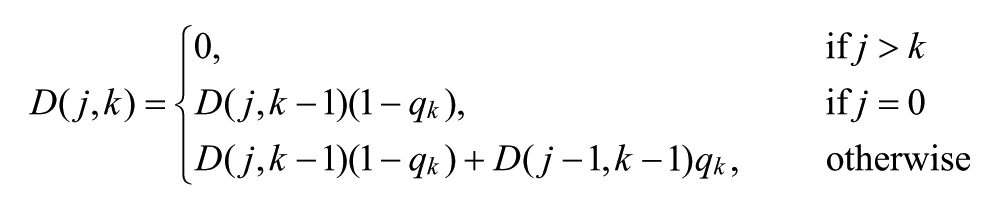
D (j, k) = {\begin{array}{l} 0, & if j > k \\ D (j, k - 1) (1 - q_{k}), & if j = 0 \\ D (j, k - 1) (1 - q_{k}) + D (j - 1, k - 1) q_{k}, & otherwise \end{array}

for $0 \leq j \leq N$ , $2 \leq k \leq N$ , where $N$ is the total number of Senate races.

Once the probabilities $D (j, k)$ have been obtained, they can be used to determine a variety of useful quantities. For example, to determine the probability that the Democratic party holds exactly 51 Senate seats after the 2012 election, the number of seats held prior to the election (in this case, 30) is first subtracted to yield the number of seats the Democrats need to gain as a result of the election (in this case, 21). The probability of the Democrats winning exactly 21 of the 33 seats that are available in the 2012 elections is $D (21, 33)$ . An identical argument holds for all possible seat counts (between 30 and 63, inclusive, because it is impossible for the Democrats to have fewer than 30 or more than 63 seats). By using this information, the probability that the Democratic party secures a simple majority in the Senate after the 2012 election can be computed as

\Pr (Democrats achieve a simple majority) = \sum_{i = 21}^{33} D (i, 33) .

With the presidential model, it suffices to compute the probabilities of the Democratic candidate (Obama) winning any specific number of electoral votes, as these probabilities can be used to compute the probabilities that the Republican candidate (Romney) wins any specific number of electoral votes. This is done by using the fact that the number of electoral votes received by Romney is 538 minus the number of electoral votes received by Obama, because these two were the only candidates with non-zero probabilities of winning any state. However, such a relationship does not hold in the Senate, or more generally, when there are more than two factions competing for the units of interest (e.g., electoral votes or Senate seats). Thus, it is necessary to compute for each party the probabilities of securing any number of Senate seats.

There is one additional complication with the Senate results, namely, that independent candidates, if elected, generally choose to caucus with one of the two major parties. This can potentially affect the balance of power in the Senate. Analyzing the possible effects of independents’ caucus choices can quickly become intractable even for a moderate number of candidates. Fortunately, for the 2012 elections there were only two independents who had a non-zero probability of winning in their respective states, and both independents were widely expected to caucus with the Democrats. Because of this, the likely size of the Democratic caucus could be determined by applying the dynamic programming algorithm with the probability of winning each seat set to the probability of the Democrat winning plus the probability of the independent winning. This approach was used for all forecasts for the 2012 and 2014 Senate races.

Senate ties

In a two-party system, a tie in the Senate can occur if both parties secure 50 seats. The probability of such an event is equal to the probability that one of the parties secures exactly 50 seats, because the other party must then secure the remaining 50 seats. However, when third-party candidates must be taken into account, the situation becomes more complicated. For example, a tie could occur with both major parties securing 50 seats, or with both major parties securing 49 seats and two seats going to independent candidates, or with both major parties securing 48 seats and four seats going to independent candidates, and so on. One way to simplify this is to make assumptions regarding the parties with which each third-party candidate will caucus, and then treat those candidates as members of the appropriate party for the purposes of determining seat totals and probabilities. As mentioned previously, in the 2012 elections, both third-party candidates who had a non-zero probability of winning their respective race were expected to caucus with the Democrats, so this simplifying step could be applied when computing the probability of a 50–50 Senate seat split between the coalition of Democrats and independents and the Republicans. Using this procedure in 2012, there was a significant probability of a tie in the Senate (between .25 and .30) during the summer (June 26 through September 16), but after September 17 this probability dropped significantly and stayed below .04 after that. In 2014, the probability of a tie remained significant throughout the election, though it started to drop in mid-October and ended at .01 in the final election day forecast.

Assumptions and Limitations

The primary assumptions made by the model of Rigdon et al. (2009) are reviewed here. The purpose of presenting these assumptions is to identify and highlight the model’s strengths and limitations. These assumptions are as follows:

The impact of race fundamentals is captured in polling data, and so these fundamentals are not explicitly incorporated into the model.

Forecasts for races are made using only race-specific polling data. Infrequently polled races are assumed to be those whose outcomes are unlikely to change.

House effects from pollsters will tend to cancel out when averaging polls for each race and so adjustments for these effects are not incorporated into the model.

Polls are representative of the actual election turnout. Any possible biases, systematic errors, or other problems within the polling data are not taken into account.

Outcomes across races are assumed to be independent, with no correlated error in the polls.

If any of these assumptions are incorrect, then the forecasts from the model will most likely be misleading or inaccurate. Other forecasting models relax or remove some of these assumptions by attempting to compensate for them, though this adds complexity to the model and has the possibility of introducing additional noise into the forecasts (Jackman, 2005; Linzer, 2013; Silver, 2012; Wang, 2012). A comparison of several models for the 2012 and 2014 elections can be found in the section “Comparisons to Other Forecasting Sites.”

Assumption 4 in particular implies that no uncertainty is added to the forecasts to account for possible problems with polls. As such, forecasts tend to be overconfident in the outcomes of individual races and consequently also in the national outcomes. Interpreting each forecast as a snapshot of the current state of the election puts the probabilities into a better perspective, where they can be viewed as estimates of likely outcomes if the election were held on that day.

Assumption 5 simplifies the process of translating race forecasts into national forecasts. For example, if $E_{i}$ ( ${\bar{E}}_{i}$ ) is the event that the Democrat wins (loses) race $i$ , then Assumption 5 guarantees that $\Pr (E_{i} | E_{j}) = \Pr (E_{i} | {\bar{E}}_{j}) = P (E_{i})$ for races $i$ and $j$ with $i \neq j$ . This does not prohibit polls from other races being used to estimate the probability of the Democrat winning in a particular race, only that the actual outcomes of other races do not influence the outcome of that race.

When Assumption 5 is valid, the dynamic programming algorithm of Kaplan and Barnett (2003) computes the exact distribution of electoral college votes whereas simulation methods that use independent coin flips for each race approximate this distribution. If this assumption is not made, then some model of dependency between the races is necessary to estimate probabilities for national outcomes from the individual races. For example, if simulation is used to approximate the distribution of electoral college votes for a candidate, then it would be necessary to know how to update the probability of the candidate winning race $i$ based on which of the preceding races he or she had won in that particular iteration.

One reason why Assumption 5 might not hold would be the presence of correlated errors within the polling data. For example, polls across all races might overstate the actual level of support for one candidate, and thus if that candidate loses in one race, then it becomes more likely that he or she will lose in the other races as well. However, Assumption 5 is made not so much because it is believed to hold, but rather because incorporating dependency between the races seems more likely to introduce noise in the forecasts if it is not modeled correctly. The fact that Assumption 5 can be used to considerably simplify the calculations of national outcomes is an added benefit. Correlated error in the polls can be partially accounted for by the various swing scenarios, which shift the proportions of undecided voters uniformly across all races. To update candidates’ polled levels of support directly, the forecasting model could be extended to include a random variable that represents global bias across all polls. Simulated draws from the distribution of this random variable could be used to update the polling data based on the sampled value, recompute the candidates’ probabilities of winning, and then apply the dynamic programming algorithm to compute the exact distribution of electoral votes or Senate seats under that particular realization of the random variable. Repeating this process many times and averaging the resulting electoral college distributions would provide one way to potentially account for the possibility of correlated error within the polls without having to explicitly model the dependency between states. An approach such as this appears to have been used by Silver (2012), though without the dynamic programming component. Relaxing Assumption 5 within the model of Rigdon et al. (2009) is a direction for future research.

Forecasts for the 2012 and 2014 Elections

Throughout the 2012 and 2014 elections, polls for the various races were monitored through the Real Clear Politics (2012) website. As new polling data became available, it was used to update the probabilities of each presidential candidate securing a majority of electoral votes and each party securing a majority of seats in the Senate and House. All forecasts were made available online (Sauppe, Jacobson, & Rigdon, 2012, 2014).

Presidential Forecasts

In 2012, the primary presidential candidates were Democrat Barack Obama, the incumbent running for his second term, and Republican Mitt Romney, the challenger. The priors for this election were constructed using the 2008 presidential election results.

Figure 4 shows a time-series plot of the probabilities of Obama winning, Romney winning, and a tie. A timeline of some of the important events in the election campaign are shown across the top of the graph. The figure indicates that Obama had a very high probability of winning at every point during the election, though Romney had a few surges. The details of the state-by-state results (based on data published on the morning of election day) are shown in Table A1 in the appendix. On the day of the election, the model correctly predicted the outcomes in 50 of the 51 states, missing only Florida, which had the smallest margin of victory (.007) of all the states.

Figure 4.

Time-series plot of the probability that each candidate will win the election from April 30, 2012, until November 6, 2012 (election day), along with a timeline of related events.

Figure 5 shows a probability histogram of the posterior distribution for the number of electoral votes for Obama on the morning of November 6, 2012. Electoral vote totals that would lead to Obama (Romney) winning are shown as blue (red) bars. The bar at 270 is black, representing the probability of a tie. Nearly all of the probability lies on the numbers greater than or equal to 270, making it virtually certain that Obama would win. Because there are so few close races, just four scenarios account for about .77 of the total probability:

303 electoral votes for Obama, probability of .46, Obama wins VA, Romney wins FL;

290 electoral votes for Obama, probability of .17, Romney wins VA, Romney wins FL;

332 electoral votes for Obama, probability of .10, Obama wins VA, Obama wins FL;

319 electoral votes for Obama, probability of .04, Romney wins VA, Obama wins FL.

Figure 5.

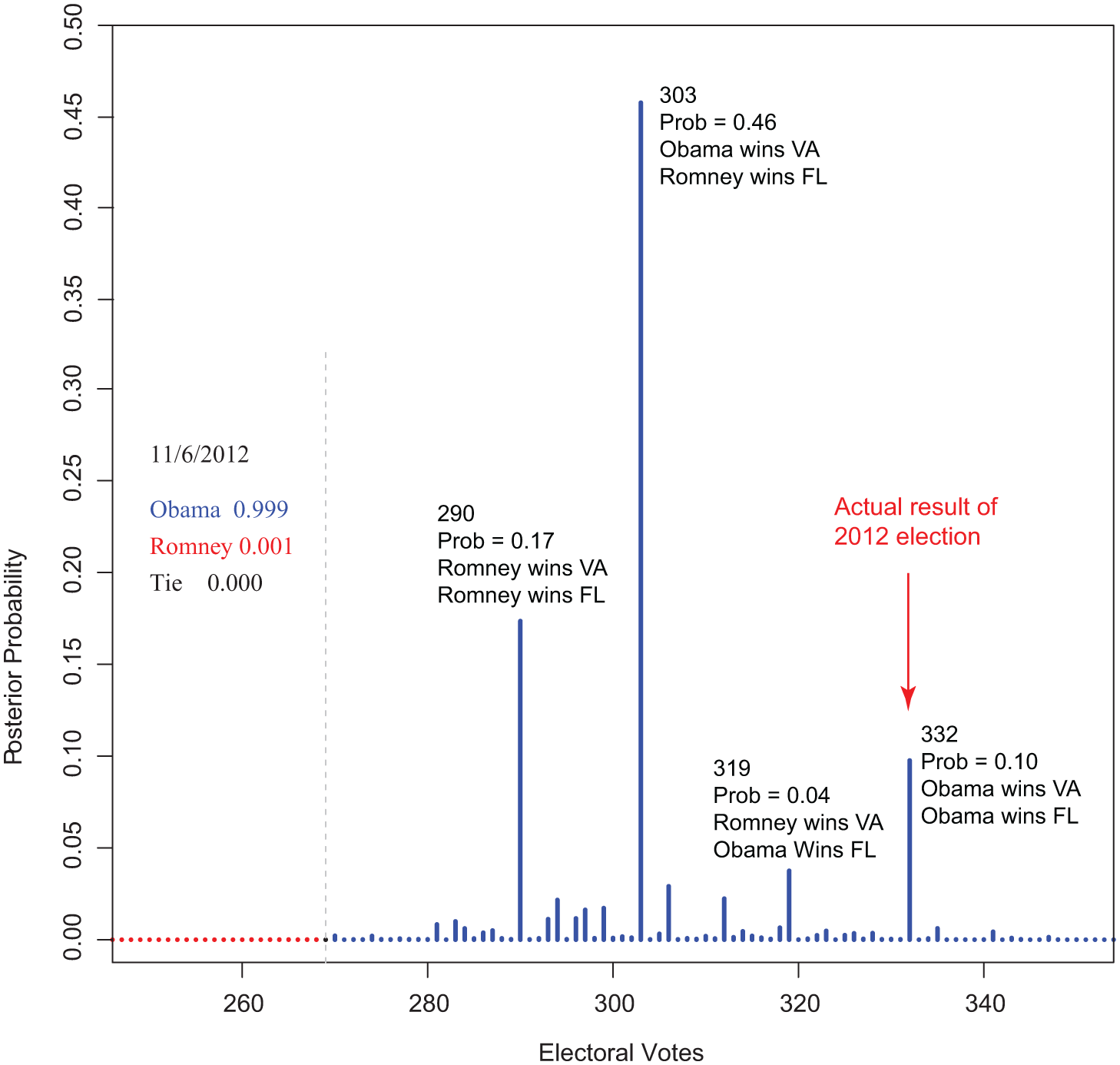
Probability histogram for 2012 election on the morning of the election.

The actual outcome of the election was the third scenario, with Obama winning 332 electoral votes. The final forecast gave an expected value of about 304 electoral votes for Obama.

Senate Forecasts in 2012

The 2012 Senate election involved 21 of the 51 seats held by the Democrats, 10 of the 47 seats held by Republicans, and both of the seats held by independents (Lieberman from Connecticut and Sanders from Vermont, both of whom caucused with the Democrats), for a total of 33 seats. Priors for each of the seats were based on the last relevant election. Table A2 in the appendix shows the race-by-race probabilities for each party on the morning of the election, along with the winning party. Of the 33 Senate races, the forecasting model correctly predicted 31 of the winners, missing only Montana (predicted Democrat/Republican probabilities of winning were .474 and .526, respectively, whereas the actual turnout was 48.8% Democrat to 44.7% Republican) and North Dakota (predicted Democrat/ Republican probabilities of winning were .135 and .865, respectively, whereas the actual turnout was 50.5% Democrat to 49.5% Republican). The Democrat Party garnered 23 seats for a post-election total of 53, the Republican Party garnered 18 for a total of 45, and independents won the remaining two seats.

Senate Forecasts in 2014

The 2014 Senate election involved 21 of the 53 seats controlled by the Democrats, 15 of the 45 seats controlled by the Republicans, and neither of the two seats held by independents (Sanders from Vermont and King from Maine, both of whom caucused with the Democrats), for a total of 36 seats. Table A3 in the appendix shows the race-by-race probabilities for each party on the morning of the election, along with the winning party. The forecasting model correctly predicted 35 of these races, missing only North Carolina (predicted Democrat/Republican probabilities of winning were .959 and .041, respectively, whereas the actual turnout was 47.3% Democrat to 49.0% Republican). The races in Louisiana and Georgia were both expected to be decided by runoff races, though this occurred only in Louisiana; in both cases the eventual winner was correctly identified. The Democrats won 12 seats while the Republicans won 24, for post-election totals of 44 seats and 54 seats, respectively.

House Forecasts in 2012

Every seat in the House was up for election in 2012. Prior to the election, the Democrats had approximately 190 seats while the Republicans had approximately 240 seats. (These totals fluctuated during the run-up to the election due to vacancies and the appointment of temporary replacements.) Due to political districting, most of these seats were considered safe for the party currently holding them.

There were several issues and limitations for the forecasts for the 2012 House races. First, the construction of priors for the House races in 2012 was complicated by the redistricting that occurred after the 2010 census. Because the previous House elections in 2010 used potentially different districts than those in 2012, it was not always clear how to use election results from 2010 races to estimate priors for the 2012 races. Because of this difficulty, all House priors were based on a combination of pundits’ subjective ratings. Second, many House races were considered to have a clear winner prior to the election so no polls were conducted for them. Even for close races, polling data were typically limited due to the difficulties associated with collecting the data. These two factors meant that the House forecasts depended heavily on the subjective priors.

House forecasts were posted on the project website from October of 2012 through election day. On the day of the election, the model correctly predicted 408 of the 435 House races, incorrectly predicted 14 races, and considered 13 races too close to call (50/50 split between candidates). The election day forecast predicted a Republican-controlled House with the Democrats securing 193 seats and the Republicans securing 242, whereas the actual election led to 201 seats for the Democrats and 234 seats for the Republicans. No House forecasts were made for 2014.

Comparisons With Other Forecasting Sites

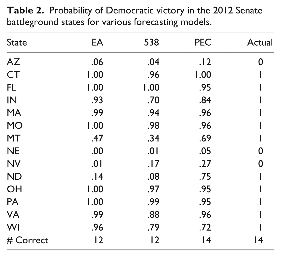
Tables 1, 2, and 3 present the election day probabilities of Democratic victories in the battleground states for the 2012 presidential election, 2012 Senate election, and 2014 Senate election, respectively, for several forecasting models. The forecasts are EA (Election Analytics; Sauppe et al., 2012, 2014), 538 (Silver, 2012, 2014), PEC (Princeton Electoral Consortium; Wang, 2012), Votamatic (Linzer, 2012, 2014), and Pollster (Boice et al., 2012; Bycoffe et al., 2014; Bycoffe et al., 2012). The Actual column indicates whether or not the Democratic candidate won the race. Probabilities for EA were taken from the project website. For all other sites, the 2012 probabilities were taken from Branwen (2012) while the 2014 probabilities were taken from the respective websites. All numbers were rounded to two decimal places. The # Correct row indicates the number of states where the probabilities favored the eventual winner. For the presidential election, both 538 and PEC are given half a point for listing Florida as essentially a toss-up.

Table 1.

Probability of Democratic victory in the 2012 presidential battleground states for various forecasting models.

State	EA	538	PEC	Votamatic	Pollster	Actual
CO	.96	.80	.84	.98	.77	1
FL	.18	.50	.50	.60	.52	1
IA	.99	.84	.84	1.00	.84	1
MI	.99	.99	1.00	1.00	1.00	1
NV	.98	.93	.99	1.00	.91	1
NH	.98	.85	.84	1.00	.83	1
NC	.01	.26	.16	.09	.28	0
OH	1.00	.91	.93	1.00	.93	1
PA	.99	.99	.93	1.00	.99	1
VA	.73	.79	.84	.98	.78	1
WI	1.00	.97	.99	1.00	.97	1
# Correct	10	10.5	10.5	11	11	11

Table 2.

Probability of Democratic victory in the 2012 Senate battleground states for various forecasting models.

State	EA	538	PEC	Actual
AZ	.06	.04	.12	0
CT	1.00	.96	1.00	1
FL	1.00	1.00	.95	1
IN	.93	.70	.84	1
MA	.99	.94	.96	1
MO	1.00	.98	.96	1
MT	.47	.34	.69	1
NE	.00	.01	.05	0
NV	.01	.17	.27	0
ND	.14	.08	.75	1
OH	1.00	.97	.95	1
PA	1.00	.99	.95	1
VA	.99	.88	.96	1
WI	.96	.79	.72	1
# Correct	12	12	14	14

Table 3.

Probability of Democratic victory in the 2014 Senate battleground states for various forecasting models. For Kansas, the independent candidate’s probability of winning is used.

State	EA	538	PEC	Votamatic	Pollster	Upshot	ELab	Actual
AK	.16	.26	.43	.23	.32	.34	.19	0
AR	.00	.04	.17	.03	.15	.11	.01	0
CO	.01	.28	.40	.22	.39	.20	.02	0
GA	.02	.25	.31	.07	.29	.33	.21	0
IA	.12	.30	.47	.25	.39	.31	.11	0
KS	.37	.53	.57	.08	.42	.49	.02	0
KY	.00	.02	.13	.03	.18	.02	.01	0
LA	.01	.19	.26	.15	.31	.15	.02	0
NH	.93	.79	.63	.59	.57	.66	.97	1
NC	.96	.69	.57	.56	.53	.71	.76	0
VA	1.00	.99	.92	.99	.97	.97	.99	1
# Correct	9	8	8	9	9	9	9	10

Table 4 provides a list of Brier scores for the election day forecasts of various models computed across all races in the election. The model of Rigdon et al. (2009) fared worst in the presidential election, due primarily to the poor prediction in Florida. For the 2012 Senate election, it performed slightly better than the model of Silver (2012) by hedging more on Montana and North Dakota, but it lost to the model of Wang (2012), which correctly predicted both of those races. In 2014, the model came in third out of seven, losing only to Linzer (2014) and Sides et al. (2014) due to a higher uncertainty in Kansas and a lower uncertainty in North Carolina.

Table 4.

Brier scores for final presidential and Senate forecasts.

Type	EA	538	PEC	Votamatic	Pollster	Upshot	ELab
President	.0147	.0091	.0076	.0039	.0097	—	—
Senate 2012	.0312	.0448	.0125	—	—	—	—
Senate 2014	.0307	.0316	.0439	.0189	.0358	.035	.0187

These results demonstrate that the model of Rigdon et al. (2009) performed competitively with other models and was able to produce accurate forecasts in almost all races in 2012 and 2014, missing only four states in the presidential and Senate elections. Thus, the assumptions discussed in section “Assumptions and Limitations” did not significantly affect the quality of the final forecasts. One limitation of this analysis is that these comparisons are for the final election day forecasts, not forecasts made in the weeks before the election. Assessing the model’s accuracy throughout the election cycle and identifying ways in which forecasts can be improved are left as directions for future research. In addition, constructing a metric for measuring the costs and increased model complexity associated with mitigating the assumptions discussed in the “Assumptions and Limitations” section will help in identifying whether or not potential improvements should be made.

Conclusion

This article describes an extension of the Bayesian model of Rigdon et al. (2009) that allows it to forecast which party will control a majority of seats in each chamber of Congress. The model uses race-specific polls to estimate the likelihood of each candidate winning each individual race in the election. These individual race outcomes are then aggregated to assign probabilities to national outcomes of interest such as the seat totals for each political party in the U.S. Senate and House of Representatives.

The model was applied to the 2012 presidential and congressional elections and the 2014 Senate elections. Forecasts were updated throughout the election cycle and made available online. The 2012 presidential election was not close at any time, with Obama’s probability of winning exceeding .80 throughout most of the presidential campaign. On the morning of election day, the probability that Obama would win the election was estimated to exceed .999. In contrast, the model indicated a close 2012 Senate election until mid-September, at which point Democratic control was expected with high probability up through election day. For 2014, the model indicated a close race through mid-September, after which the Republicans were increasingly favored to take control of the Senate.

Footnotes

Appendix

Table A3.

Final race probabilities (including possibility of runoffs) for Senate seats on the morning of the 2014 election, along with the winning party. The number of general election polls in each race, the date of the last poll, and the margin of victory (computed as the difference between the vote fractions of the winning candidate and the runner-up) are also shown. The margin of victory for Louisiana is taken from the runoff race.

State	Probability of winning			Winner	Correct?	No. of polls	Date of last poll	Margin of victory
State	Democrat	Republican	Independent	Winner	Correct?	No. of polls	Date of last poll	Margin of victory
Alabama	—	1.000	—	R	Yes	0	NA
Alaska	.160	.840	—	R	Yes	20	November 2, 2014	.036
Arkansas	.000	1.000	—	R	Yes	36	November 1, 2014	.17
Colorado	.010	.990	—	R	Yes	37	November 2, 2014	.041
Delaware	1.000	.000	—	D	Yes	5	October 23, 2014	.136
Georgia	.020	.980	—	R	Yes	33	November 3, 2014	.079
Hawaii*	1.000	.000	—	D	Yes	7	October 23, 2014	.421
Idaho	.000	1.000	—	R	Yes	6	October 23, 2014	.306
Illinois	1.000	.000	—	D	Yes	13	November 2, 2014	.099
Iowa	.120	.880	—	R	Yes	45	November 3, 2014	.085
Kansas	.000	.630	0.374	R	Yes	19	November 3, 2014	.108
Kentucky	.000	1.000	—	R	Yes	34	November 1, 2014	.155
Louisiana	.010	.990	—	R	Yes	20	November 1, 2014	.119
Maine	.000	1.000	—	R	Yes	15	November 2, 2014	.369
Massachusetts	1.000	.000	—	D	Yes	15	November 1, 2014	.239
Michigan	1.000	.000	—	D	Yes	64	November 2, 2014	.132
Minnesota	1.000	.000	—	D	Yes	18	October 30, 2014	.102
Mississippi	.000	1.000	—	R	Yes	8	October 23, 2014	.23
Montana	.000	1.000	—	R	Yes	5	October 23, 2014	.179
Nebraska	.000	1.000	—	R	Yes	6	October 23, 2014	.338
New Hampshire	.930	.070	—	D	Yes	49	November 3, 2014	.033
New Jersey	1.000	.000	—	D	Yes	15	November 2, 2014	.142
New Mexico	1.000	.000	—	D	Yes	10	October 23, 2014	.107
North Carolina	.960	.040	—	R	No	64	November 3, 2014	.017
Oklahoma	.000	1.000	—	R	Yes	8	October 29, 2014	.395
Oklahoma*	.000	1.000	—	R	Yes	8	October 29, 2014	.389
Oregon	1.000	.000	—	D	Yes	16	October 27, 2014	.179
Rhode Island	1.000	.000	—	D	Yes	4	October 23, 2014	.41
South Carolina	.000	1.000	—	R	Yes	9	October 23, 2014	.156
South Carolina*	.000	1.000	—	R	Yes	7	October 23, 2014	.241
South Dakota	.000	1.000	0.000	R	Yes	16	October 26, 2014	.209
Tennessee	.000	1.000	—	R	Yes	6	October 23, 2014	.301
Texas	.000	1.000	—	R	Yes	10	October 23, 2014	.272
Virginia	1.000	.000	—	D	Yes	21	October 29, 2014	.008
West Virginia	.000	1.000	—	R	Yes	12	October 23, 2014	.276
Wyoming	.000	1.000	—	R	Yes	5	October 23, 2014	.547

Note. R = Republican; D = Democrat. *Special elections.

Acknowledgements

The authors would like to thank Angela Mengke Ding, Taylor Fairbank, Bhargava Manja, Calvin Shipplett, and Dimitriy Zavelevich for their work on improving the Election Analytics website, as well as Joshua Gluck for assistance with improving the code for computing the Bayesian posterior probabilities. The authors would also like to thank Dr. Dino Christenson, the article editor, and two anonymous reviewers for feedback and comments, which led to a considerable improvement in the article.

Declaration of Conflicting Interests

The author(s) declared no potential conflicts of interest with respect to the research, authorship, and/or publication of this article.

Funding

This research has been supported in part by the Department of Defense (DoD) through the National Defense Science & Engineering Graduate Fellowship (NDSEG) Program (32 CFR 168a) and the National Science Foundation Graduate Research Fellowship Program (DGE-1144245).

Author Biographies

Steven E. Rigdon is professor of Biostatistics in the College for Public Health and Social Justice at Saint Louis University. He is also distinguished research professor emeritus at Southern Illinois University Edwardsville. His research interests include bayesian statistics, disease surveillance, election monitoring, and applications in sports.

Jason J. Sauppe is a PhD candidate in the Department of Computer Science at the University of Illinois at Urbana-Champaign. His research interests include optimization and operations research.

Sheldon H. Jacobson is a professor of Computer Science at the University of Illinois at Urbana-Champaign. His research interests are in the area of operations research, with applications in public policy, public health, and sports. He is a Fellow of INFORMS and IIE.

References

Boice

Bycoffe

Scheinkman

(2012). Pollster: 2012 Presidential forecasts. Retrieved from http://elections.huffingtonpost.com/2012/romney-vs-obama-electoral-map

Branwen

(2012). 2012 election predictions. Retrieved from http://www.gwern.net/2012%20election%20predictions

Brown

L. B.

Chappell

H. W.

Jr. (1999). Forecasting presidential elections using history and polls. International Journal of Forecasting, 15, 127-135.

Bycoffe

Boice

Fung

(2014). Pollster: 2014 Senate forecasts. Retrieved from http://elections.huffingtonpost.com/2014/senate-outlook

Bycoffe

Carlson

Boice

Scheinkman

(2012). Pollster: 2012 Senate forecasts. Retrieved from http://elections.huffingtonpost.com/2012/senate-outlook

Christensen

W. F.

Florence

L. W.

(2008). Predicting presidential and other multistage election outcomes using state-level pre-election polls. The American Statistician, 26, 1-10.

Cox

Katz

(2014). The upshot: 2014 Senate forecasts. Retrieved from http://www.nytimes.com/newsgraphics/2014/senate-model/

Jackman

(2005). Pooling the polls over an election campaign. Australian Journal of Political Science, 40, 499-517.

Kaplan

E. H.

Barnett

(2003). A new approach to estimating the probability of winning the presidency. Operations Research, 51, 32-40.

10.

Linzer

D. A.

(2012). Votamatic: 2012 Presidential forecasts. Available from http://votamatic.org

11.

Linzer

D. A.

(2013). Dynamic Bayesian forecasting of presidential elections in the states. Journal of the American Statistical Association, 108, 124-134.

12.

Linzer

D. A.

(2014). Votamatic: 2014 Senate forecasts. Retrieved from http://www.dailykos.com/election-outlook/2014-senate

13.

Real Clear Politics. (2012). Available from http://www.realclearpolitics.com

14.

Rigdon

S. E.

Jacobson

S. H.

Cho

W. K. T.

Sewell

E. C.

Rigdon

C. J.

(2009). A Bayesian Prediction Model for the U.S. presidential election. American Politics Research, 37, 700-724.

15.

Sauppe

J. J.

Jacobson

S. H.

Rigdon

S. E.

(2012). Election analytics: 2012 forecasts. Available from http://election12.cs.illinois.edu

16.

Sauppe

J. J.

Jacobson

S. H.

Rigdon

S. E.

(2014). Election analytics: 2014 Senate forecasts. Available from http://electionanalytics.cs.illinois.edu

17.

Sides

Elliot

Nelson

Pezon

(2014). Election lab 2014. Retrieved from http://www.washingtonpost.com/wp-dre/politics/election-lab-2014

18.

Silver

(2012). FiveThirtyEight: 2012 forecasts. Available from http://fivethirtyeight.blogs.nytimes.com

19.

Silver

(2014). FiveThirtyEight: 2014 Senate forecasts. Retrieved from http://fivethirtyeight.com/interactives/senate-forecast/

20.

Wang

(2012). Princeton Electoral Consortium. Available from http://election.princeton.edu

Forecasting the 2012 and 2014 Elections Using Bayesian Prediction and Optimization

Abstract

Keywords

Introduction

Background

The Forecasting Model

The Bayesian Model

Priors and polling data

Computing a candidate’s probability of winning

Additional considerations

The Dynamic Programming Algorithm

The Senate algorithm

Senate ties

Assumptions and Limitations

Forecasts for the 2012 and 2014 Elections

Presidential Forecasts

Senate Forecasts in 2012

Senate Forecasts in 2014

House Forecasts in 2012

Comparisons With Other Forecasting Sites

Conclusion

Footnotes

Appendix

Acknowledgements

Declaration of Conflicting Interests

Funding

Author Biographies

References