Sage Journals: Discover world-class research

Abstract

Examining the relationship between renewable and non-renewable energy sources and economic growth is crucial for designing sustainable growth policies in the context of global sustainability efforts. Previous studies relying on frequentist inference have faced challenges in disentangling the individual effects of these energy sources on economic growth due to their high degree of correlation, often leading to biased results. The Bayesian approach offers an alternative estimation method to address this multicollinearity issue. This study aims to demonstrate one of the advantages of the Bayesian hierarchical framework in handling multicollinearity by using a sample of 72 countries to evaluate the distinct impacts of renewable and non-renewable energy on economic growth. By incorporating specific priors into a Bayesian model to guide the estimation process, the findings confirm that both energy sources play significant roles in driving economic growth, with renewable energy sources exhibiting a comparatively weaker effect. These results align with theoretical expectations, indicating that renewables make a limited contribution to economic growth due to high investment costs, intermittency issues, and supply chain constraints. This study establishes a solid foundation for sustainable growth policy formulation by providing robust evidence.

Plain language summary

In studying the energy-growth nexus, the Bayesian approach offers a robust and reliable estimation method to address multicollinearity issues, which makes it impossible for frequentist methods. The study aims to demonstrate one of the advantages of the Bayesian hierarchical framework in handling multicollinearity on a sample of 72 countries to access energy on economic growth. Renewable and non-renewable energy sources are significant drivers of economic growth, but renewable energy sources exert a comparatively weaker effect. These results are consistent with theoretical expectations that renewables make a limited contribution to economic growth owing to high investment costs, intermittency issues, and supply chain constraints. The study provides a robust empirical foundation for sustainable growth policy formulation. The main limitation of the study is the use of empirical rather than informative priors.

Keywords

Bayesian hierarchical model multicollinearity renewables non-renewables sustained economic growth

Introduction

Along with physical capital, human capital, and the labor force, non-renewable and renewable energy sources become fundamental factors in economic growth, as the growth hypothesis suggests. World energy consumption is projected to increase by 49% between 2007 and 2035 (U.S. Department of Energy, 2010). Non-renewable energy sources, being less costly, currently dominate energy production and consumption, accounting for approximately 80% of global energy consumption (REN21, 2019). Global concerns related to environmental pollution, volatile prices of non-renewable sources, the risk of depletion, energy security, and heavy reliance on imported energy highlight the need for investments in renewable sources. Countries worldwide have been transitioning toward renewable energy generation and usage, expecting to contribute to sustainable growth. However, designing a sustainable growth policy encounters challenges because of the lack of reliable empirical findings obtained through earlier frequency-based research on the energy-growth nexus. Some studies analyzed the impact of aggregated energy consumption on economic growth (Acaravci & Ozturk 2010; Ang, 2007; Apergis & Payne, 2009; Chien-chiang, 2005; Guo, 2018; Huang et al., 2008; Kasman & Duman, 2015; Kraft & Kraft, 1978; Lee & Chang, 2008; Mehrara, 2007; Tang et al., 2016; Uçan et al., 2022), some focused on the impact of renewable or non-renewable energy consumption on economic growth (Apergis & and Payne, 2010; Al-Mulali et al., 2013; Awodumi & Adeleke, 2016; Awodumi & Adewuyi, 2020; Bildirici & Bakirtas, 2014; Bhattacharya et al., 2016; Dabboussi & Abid, 2022; Koçak & Şarkgüneşi, 2017; Ntanos et al., 2018; Ozcan & Ozturk, 2019; Paramati et al., 2017; Sun-Park & Yoo, 2014; Yildirim et al., 2012), and others aimed to include both renewable and non-renewable variables in a single regression model (Apergis & Payne, 2011a, 2011b; Al-Mulali et al., 2014; Destek & Aslan, 2017; Jebli & Youssef, 2015; Okumus et al., 2021; Ozturk et al., 2022; Tugcu et al., 2012; Ummalla & Samal, 2019). However, these approaches do not allow for the identification of the individual effects of renewable and non-renewable energy consumption, often leading to unreliable estimation outcomes. One critical issue in analyzing the relationship between renewable and non-renewable energy and economic growth variables addressed in this study is the presence of multicollinearity. Multicollinearity refers to a high degree of correlation among independent variables and can cause problems in econometrics, as it violates certain assumptions and leads to unreliable and unstable estimates. In this case, the high correlation (above 0.8) between renewable and non-renewable variables can potentially result in multicollinearity, making it challenging to disentangle these variables’ individual effects as they become confounded by shared factors. The studies mentioned above used frequentist methods, representing different but potentially biased approaches. Running separate regressions for either renewable or non-renewable variables may introduce an omitted variables bias. Conversely, using conventional frequentist estimation, including both renewable and non-renewable variables in a model, may lead to biased effects due to their high correlation. This issue of confounding renewable and non-renewable effects may contribute to the contradictory findings observed in analyses of the energy-growth causality. While frequentist methods, such as ordinary least squares (OLS) regression, do not directly address multicollinearity issues, several remedial measures can be employed to mitigate the problem. It is worth noting that Bayesian methods, which take a different approach to statistical inference, offer more flexible solutions to multicollinearity issues (Block et al., 2011; Hahn & Doh, 2006; Leamer, 1973). Bayesian regression models can incorporate prior information and utilize hierarchical models to address multicollinearity.

From the above analysis, the study aims to demonstrate the advantages of employing a Bayesian approach over traditional frequentist inference when addressing multicollinearity issues. To this end, this research employs a Monte Carlo simulation study to separate the effects of renewable and non-renewable energy consumption on economic growth within a single model, using a Bayesian hierarchical regression on a panel dataset consisting of 72 countries. The study contributes to the existing knowledge on energy-growth relationships. First, our research is pioneering in using a Bayesian hierarchical model to disentangle the individual effects of renewables and non-renewables on economic growth. By specifying informative prior settings that contain specific information about key parameters for renewables and non-renewables, we can encode our beliefs regarding the interactions and impact directions between these predictors and the response variable. Second, thanks to the Bayesian approach’s capacity to incorporate our beliefs and prior knowledge about the relationships among variables, this study effectively manages multicollinearity and reveals a strong positive association between both types of energy and economic growth, with non-renewables exerting a more substantial effect compared to renewables. Third, the precise and robust findings obtained from thoughtful Bayesian inference emphasize the critical need to accelerate the transition to sustainable energy for global economic growth.

The study is organized into the following sections. In section “Introduction,” the motivation, aim, and contribution of the research are clarified. Four hypotheses and empirical investigations on the relationship between energy and economic growth are analyzed in section “Literature review.” Section “Methodology, model, and data” introduces the methodology, model, and data. Bayesian simulation outcomes are presented and interpreted in section “Bayesian simulation outcomes.” The last section provides conclusions, recommendations, and limitations of the study.

Literature Review

Four Hypotheses on the Energy-Growth Nexus

The investigation of the causal relationship between energy and economic growth can be traced back to Kraft and Kraft’s study in 1978. Over the past five decades, the literature on this topic has experienced significant development, as evidenced by surveys conducted by Ozturk (2010), Omri (2014), Ahmad et al. (2020), and Mutumba et al. (2021) focusing on sustainability. In the energy literature, the relationship between energy and growth is commonly examined through four testable hypotheses: (1) the growth hypothesis (one-way causality from energy use to economic growth), (2) the conservation hypothesis (one-way causality from economic growth to energy use), (3) the feedback hypothesis (two-way causality between energy use and economic growth), and (4) the neutrality hypothesis (the absence of causality between energy use and economic growth).

Empirical Literature

Early empirical studies predominantly conducted aggregated analyses, exploring the causal link between total energy consumption and economic growth. Subsequently, research on energy-growth relationships took two major directions. The first approach examined the separate effects of renewable and non-renewable energy consumption using individual models (Awodumi & Adeleke, 2016; Awodumi & Adewuyi, 2020; Bildirici & Bakirtas, 2014; Chen et al., 2023; Dabboussi & Abid, 2022; Hassan, Khan et al., 2022; Hassan, Song et al., 2022; Khan & Liu, 2023; Zang et al., 2023; Khan et al., 2023; Liu et al., 2023; Ntanos et al., 2018; Paramati et al., 2017; Sadorsky, 2009; Yildirim et al., 2012; Zuin et al., 2023, and many others). The second approach explored the effects of both energy types in a single model (Apergis & Payne, 2011a, 2011b; Al-Mulali et al., 2014; Jebli & Youssef, 2015; Destek & Aslan, 2017; Okumus et al., 2021; Ozturk et al., 2022; Tugcu et al., 2012; Ummalla & Samal, 2019, and many others). Given the primary focus of our study, we align with the second direction.

Apergis and Payne (2011a) employed heterogeneous panel cointegration procedures and found a positive relationship between renewable and non-renewable energy consumption and economic growth in a panel of 80 countries. Similarly, in another panel analysis of 16 emerging market economies, Apergis and Payne (2011b) observed a positive impact of renewable and non-renewable energy consumption on economic growth. Tugcu et al. (2012) investigated the connection between renewable and non-renewable energy consumption and economic growth, yielding mixed results. They found a significant positive relationship between non-renewable energy consumption and economic growth only for Japan. In contrast, no significant relationship was observed for renewable energy consumption in Canada, France, Italy, and the USA. Al-Mulali et al. (2014) employed the panel Dynamic Ordinary Least Squares (DOLS) test to demonstrate the positive impacts of renewable and non-renewable electricity consumption, fixed investment, labor, and trade on GDP growth in eight Latin American countries between 1980 and 2010. Salim et al. (2014) utilized the Common Correlated Effects Mean Group estimator to analyze the association between renewable and non-renewable energy use and GDP growth in 29 OECD countries from 1990 to 2012, revealing a positive correlation between both types of energy and GDP, with non-renewable energy exerting a more substantial effect. Jebli and Youssef (2015) employed long-run OLS, fully modified OLS, and dynamic OLS techniques to investigate 69 countries between 1980 and 2010 and concluded that both renewable and non-renewable energy consumption and trade positively affect economic growth. Kahia et al. (2017), using the panel Error Correction Model, identified positive significant elasticities among real GDP, renewable energy consumption, non-renewable energy consumption, real fixed investment, and the labor force in a sample of eleven MENA net oil-importing countries (NOICs) during the period 1980 to 2012. Zafar et al. (2019), employing the Continuously Updated Fully Modified Ordinary Least Square (CUP-FM) approach, found a promoting role of renewable and non-renewable energy consumption in economic growth across the Asia-Pacific Economic Cooperation (APEC) countries from 1990 to 2015. Ummalla and Samal (2019), focusing on China and India as influential economies, obtained mixed results using Granger causality, autoregressive distributed lag bounds testing, and vector error correction model (VECM) techniques. They found a positive impact of renewable energy consumption on economic growth in India, while no causality was confirmed for China. Additionally, they found a positive impact of natural gas consumption on economic growth in China, while no causality was found for India. Shahbaz et al. (2020) analyzed a panel of 38 renewable-energy-consuming countries from 1990 to 2018 using dynamic OLS, fully modified OLS, and heterogeneous non-causality approaches and identified the positive effects of renewable energy, non-renewable energy, capital, and labor on economic growth. Okumus et al. (2021) employed the Cross-sectional Augmented Autoregressive Distributed Lag (CSARDL) method and found evidence supporting the positive effects of renewable and non-renewable energy consumption on economic growth in G7 countries from 1980 to 2016. Furthermore, the study revealed that non-renewable energy consumption had a more significant effect than renewable energy consumption. The findings of Okumus et al. (2021) are consistent with those of Zafar et al. (2019), Rahman and Velayutham (2020), Vural (2020), and Pegkas (2020).

Most studies reviewed above collectively demonstrate the positive effects of renewable and non-renewable energy consumption on economic growth. However, there are some contrasting findings, such as those presented by Destek (2016) and Asiedu et al. (2021). Destek (2016) and Asiedu et al. (2021) found evidence supporting a positive effect of renewable energy consumption and a negative effect of non-renewable energy consumption on economic growth. Similarly, Destek and Aslan (2017), utilizing bootstrap panel causality for a panel of 17 emerging economies between 1980 and 2012, found no causality between renewable energy consumption and economic growth for 12 emerging economies, while no significant relationship was observed between non-renewable energy consumption and economic growth in nine emerging economies. Ozturk et al. (2022), using Granger causality and panel vector autoregression analysis for 20 Paris Club countries from 1991 to 2016, found no causality between fossil fuels and renewable energy consumption and economic growth.

Given the high correlation between renewable and non-renewable energy consumption, earlier studies utilizing traditional frequentist methods have yielded diverse and sometimes conflicting outcomes. In tackling this challenge of multicollinearity, the Bayesian approach offers a flexible framework. Our analysis employs a Bayesian hierarchical regression on a panel encompassing 72 countries, allowing us to derive significant conclusions: Firstly, through the incorporation of informative prior settings designed to encapsulate the specific relationships between variables in the model, the Bayesian methodology unequivocally demonstrates its superiority over frequentist estimation in managing multicollinearity. Secondly, our Bayesian results confirm that renewable and non-renewable energy sources positively contribute to economic growth. Thirdly, an interval hypothesis test conducted within the Bayesian context asserts that non-renewables substantially influence economic growth more than renewables. This finding underscores the substantial challenges that the world must overcome to expedite its transition toward sustainable economic growth.

Methodology, Model, and Data

Bayesian Monte-Carlo Algorithm

The Bayesian approach has gained popularity since the 1990s, mainly due to advancements in computer technology and software packages. Initially utilized in decision theory and macroeconomics, Bayesian statistics has expanded its application to various social disciplines (Briggs, 2023; Kreinovich et al., 2019; Nguyen, 2023; Thach et al., 2019, 2022). The growing popularity and accessibility of the Bayesian framework can be attributed to its advantages over traditional frequentist approaches.

Firstly, Bayes’ theorem, a fundamental rule of probability, can be applied to all parametric models. Additionally, Bayesian methods offer flexibility in handling complex models that may exceed the inferential capabilities of frequentist approaches. Moreover, allowing for the inclusion of all independent variables in a regression model, the Bayesian approach provides probabilistic statements about their impact on the response variable. In contrast, frequentist methods focus solely on statistically significant estimates, disregarding potentially meaningful variables that could influence the response. Furthermore, Bayesian estimation provides an entire distribution function of plausible parameter values, whereas frequentist analyses yield point estimates that are either significant or not. Owing to such flexibility, the Bayesian approach enables probability statements such as “The probability of a negative effect of a predictor on the response is 90%.”

In particular, the Bayesian approach, through integrating prior knowledge and data in econometric analysis, addresses data-related issues arising in frequentist analyses, such as multicollinearity. In frequentist regressions, the estimated coefficients are obtained by minimizing the sum of squared residuals to find the best-fitting line that minimizes the discrepancy between observed and predicted values. In multicollinearity, frequentist methods encounter challenges to disentangle the effects of highly correlated variables, leading to unstable and unreliable coefficient estimates. Coefficients may exhibit unexpected signs or magnitudes, rendering interpretation challenging. When variables are strongly correlated, distinguishing the specific contributions of each independent variable to the dependent variable becomes difficult, even impossible, as their effects become intertwined. Notably, multicollinearity can also impact the standard errors of estimated coefficients. Standard errors are crucial for assessing the precision of coefficient estimates, calculating confidence intervals, and conducting hypothesis tests. In the presence of multicollinearity, standard errors tend to be inflated. In situations where multicollinearity exists in the model, Leamer (1973), Hahn and Doh (2006), and Block et al. (2011) have recommended employing Bayesian statistics, which offer a more refined approach to econometric modeling. Using Bayesian methods contributes significantly to the energy literature, which, as discussed above, often yields contradictory findings. Bayesian methods offer two key advantages in this regard:

Firstly, the Bayesian approach provides more intuitive explanations and is aligned with theoretical expectations. Rather than making a categorical claim about whether renewable and non-renewable energy consumption positively affects economic growth, Bayesian analysis produces probability distributions that represent the likelihood of these two energy types having a positive impact on growth. By considering the data and prior information, Bayesian analysis outputs a posterior probability distribution that captures the effect of the independent variables of interest.

Secondly, Bayesian methods are more robust against multicollinearity issues than frequentist statistics (Block et al., 2011; Hahn & Doh, 2006; Leamer, 1973). Multicollinearity typically arises from insufficient data. When renewable and non-renewable variables are perfectly correlated, it becomes challenging for frequentist and Bayesian methods to separate their effects. However, Bayesian methods hold an advantage when the correlation between the independent variables reaches a high level, complicating the frequentist approach. The capability of Bayesian statistics in encoding the relationships among variables allows for the separation of the impacts of the independent variables on economic growth, suggesting that their magnitudes of influence differ.

Model Specification and Data Description

Mimicking Apergis and Payne (2011a), Al-Mulali et al. (2014), Salim et al. (2014), Kahia et al. (2017), Ummalla and Samal (2019), and Ozturk et al. (2022), we selected real GDP as the dependent variable and renewable energy, non-renewable energy, capital, and labor as the independent variables for our Bayesian regression model. However, unlike most previous studies, we introduced an additional independent variable: human capital. This addition is motivated by the recognition that physical capital, labor, and human capital are three fundamental factors in growth theory (Mankiw et al., 1992). The predictors of interest in our model are renewables and non-renewables, while physical capital, labor, and human capital are included as control variables.

Our Bayesian random-intercept (hierarchical) model is specified as follows:

\begin{matrix} GD P_{i, t} = a_{0} + a_{1} . RE C_{i, t} + a_{2} . NE C_{i, t} + a_{3} . K_{i, t} \\ + a_{4} . L_{i, t} + a_{5} . H_{i, t} + α . u + ε_{i, t} . \end{matrix}

(1)

where i (1, 2, … 72) represents the index of countries, and t denotes the research period from 1965 to 2019. REC is a proxy for the renewable share, while NEC represents the non-renewable share in primary energy, obtained from Statistical Review of World Energy and Our World in Data. K is the stock of physical capital at constant 2017 national prices (in mil. 2017US$), and GDP is proxied by real GDP at constant 2017 national prices (in mil. 2017US$). L is the number of persons engaged (in millions), and H is the human capital index based on years of schooling and returns to education. GDP, K, L, and H data are sourced from the Penn World Table, version 10.01 (PWT 10.01) (Table 1). Furthermore, a represents a vector of coefficients, α is a coefficient, u denotes the random deviations, and ε is the error term.

Table 1.

Explaining Variables in the Bayesian Hierarchical Model.

Variables	Proxies	Period	Notation	Data source
Dependent
Economic growth	Real GDP at constant 2017 national prices (in mil. 2017US$)	1965–2019	$GDP$	PWT 10.01
Independent
Physical capital	Stock of physical capital at constant 2017 national prices (in mil. 2017US$)	1965–2019	$K$	PWT 10.01
Labor force	Number of persons engaged (in millions)	1965–2019	$L$	PWT 10.01
Human capital	Human capital index	1965–2019	$H$	PWT 10.01
Renewable energy	Non-renewable share in primary energy	1965–2019	$REC$	Statistical Review of World Energy, Our World in Data (2022)
Non-renewable energy	Non-renewable share in primary energy	1965–2019	$NEC$	Statistical Review of World Energy, Our World in Data (2022)

The study utilizes an unbalanced panel comprising 72 countries, with data on renewable and non-renewable energy consumption available from 1965 to 2019. However, for certain transition countries, energy data are only available from 1985 (Azerbaijan, Belarus, Estonia, Kazakhstan, Latvia, Lithuania, Russia, Turkmenistan, Ukraine, Uzbekistan) and from 1990 (Croatia, Slovenia). Bangladesh is an exception, with its energy data accessible from 1971.

It is important to note that prior specification plays a crucial role in Bayesian simulation. Prior distributions are categorized into three types for Bayesian estimation: naïve, thoughtful (specific), and empirical (data-dependent) (Smid et al., 2020). Thoughtful Bayesian estimation occurs when at least one prior distribution is informative (Smid et al., 2020). Smid et al. (2020) emphasize that research incorporating empirical or even naïve priors can be considered within a thoughtful framework if justifiable under certain conditions. Highly informative priors play a significant role in shaping posterior probabilities, thereby influencing the entire estimation process. In cases where there is no or limited prior information or belief about model parameters, eliciting empirical priors, as suggested by Wasserman (2000), Darnieder (2011), and Martin and Walker (2019), is appropriate. McNeish (2016), van Erp et al. (2018), and Thach (2023) have concluded that Bayesian estimation using empirical prior distributions outperforms frequentist and naïve Bayesian estimators. Moreover, it has been found that variance parameters are more biased than structural parameters (McNeish, 2016). Applying half-Cauchy or Inverse Gamma priors for variance components in Bayesian analysis yields more precise estimates than other priors (McNeish & Stapleton, 2016). Van de Schoot et al. (2015) recommend using either a very informative Inverse Gamma (0.5, 0.5) or a non-informative Inverse Gamma (0.01, 0.01) for variance parameters.

We assign normal priors to the structural parameters of interest, REC and NEC for our Bayesian Monte-Carlo simulation. The prior means of the normal distributions are derived from the standard mixed-effects regression. To identify a Bayesian hierarchical model with the least uncertainty, we specify and compare three types: a random-effects model, a full mixed-effects model, and a simple mixed-effects model. A sensitivity analysis via the Deviance Information Criterion (DIC) is performed to choose the best fit. DIC is a statistical measure used in Bayesian model selection and comparison and is designed to strike a balance between the goodness of fit of a model and its complexity. It helps in model selection by considering how well the model fits the data and how complex it is. The main idea is to find a model that adequately explains the data without being overly complex or prone to overfitting. DIC is calculated using the following formula:

DIC = D_bar + p_D

(2)

where D_bar as the average posterior deviance, which is a measure of how well the model fits the data, is calculated as the average deviance over all posterior samples, p_D is the effective number of parameters, which takes into account both the complexity of the model and how well it fits the data.

Furthermore, the second sensitivity analysis is conducted to find a more appropriate prior variance for the key parameters, REC and NEC. Following Van de Schoot et al. (2015), we specify Inverse Gamma (0.5, 0.5) and non-informative Inverse Gamma (0.01, 0.01) for the overall variance. The third sensitivity analysis of the estimation results examines how the posterior conclusions are sensitive to various prior specifications. Specifically, we will vary the value of the prior variance for REC and NEC in the range of 10,000 to 1. Moreover, we will vary the prior means from −0.5 to 0.5 with an even interval of 0.1. This analysis will examine the log marginal-likelihood and posterior point and interval estimates. In Bayesian Monte Carlo Markov Chain (MCMC) simulation, the log marginal-likelihood (also known as the log evidence or the log marginal probability) is also a measure of the goodness of fit of a model to the observed data, given the model’s parameters. It plays a crucial role in Bayesian model selection and comparison. A higher log marginal likelihood indicates a better fit for the model. The log marginal likelihood is obtained by integrating the product of the likelihood function and the prior distribution over the parameter space. Mathematically, it is defined as:

logp (D | M) = \log \int^{p} (D | θ, M) p (θ | M) d θ,

(3)

where D represents the observed data, M is the model under consideration, θ denotes the parameters of the model, p(D|θ,M) is the likelihood function that describes the probability of observing the data D given the model parameters θ, and p(θ|M) is the prior distribution over the parameters, reflecting our beliefs about the parameters before observing the data.

Most importantly for this study, to compare the goodness of fit between the Bayesian mixed-effects and frequentist mixed-effects models in handling multicollinearity, we will consider the percentage of outliers in total fitted observations and the percentage of actual data within predictive intervals. Lower rates indicate a better model fit.

The explicit availability of the posterior distribution is often limited in Bayesian analysis. To overcome this, MCMC algorithms are commonly employed in simulation studies to simulate complex posterior models. In our analysis, we utilize MCMC simulations to obtain parameter estimates. During the simulation process, we specify a default MCMC sample, discarding the first 2,500 burn-in iterations from the MCMC sample. In order to assess MCMC convergence in a high-dimensional regression, we employ a thinning of 300. As a result, 3,002,201 iterations are conducted for the MCMC algorithm. Before drawing inferences, it is essential to conduct convergence tests for the MCMC algorithms. Once MCMC convergence is acquired, all model parameters will converge to plausible values.

Bayesian Simulation Outcomes

Model Comparison and Selection

The outcome of the first sensitivity analysis, as determined by the DIC values (Table 2), suggests that the Bayesian random-intercept model outperforms the other two Bayesian candidate models. Therefore, we will proceed with running this model for further analysis.

Table 2.

Model Comparison Based on DIC Estimates.

Bayesian hierarchical models	DIC estimates
Simple mixed-effects	75,793.4
Random-intercept	−2,393.407
Full mixed-effects	5,253.533

Source. Calculations by the author.

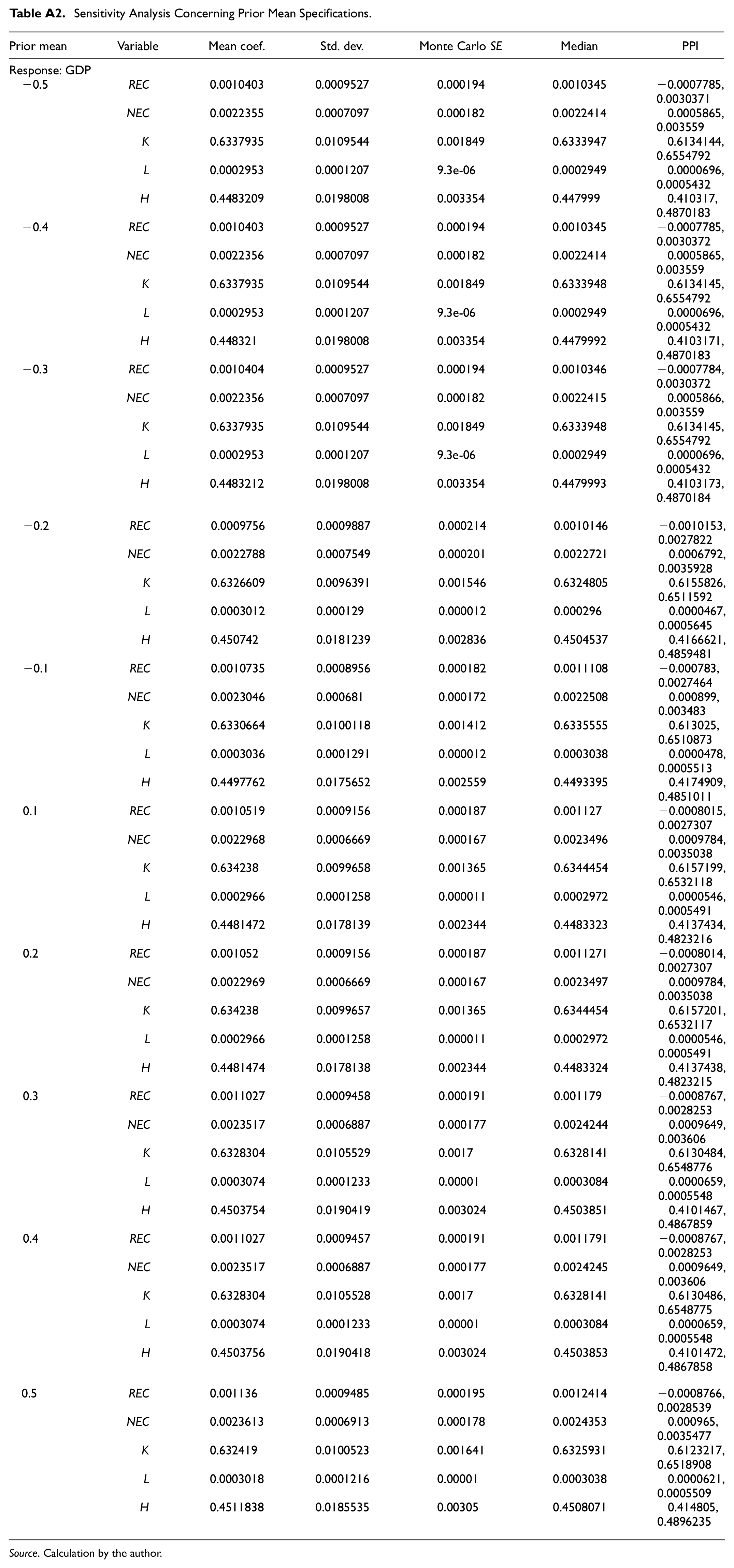
Regarding the REC and NEC parameters of the chosen Bayesian hierarchical model, we find that their posterior estimates remain consistent across a range of prior variances, ranging from 10,000 to 1 (Appendix A, Table A1). Additionally, varying the prior mean of the normal distributions within the range of −0.5 to 0.5 with a fixed prior variance does not considerably impact the posterior conclusions (Appendix A, Table A2). Our analysis reveals that the log marginal likelihood increases as the prior variance decreases, indicating that a narrower variance results in a better fit (Table 3). Consequently, the Bayesian random-intercept model with a prior variance of 1 for both REC and NEC parameters demonstrates the best performance.

Table 3.

Variance Specifications and Log Marginal-Likelihood in Naïve and Thoughtful Bayesian Estimation.

Prior variance specification	10,000	1,000	100	50	30	10	5	3	1
Log marginal-likelihood	899.7	900.0	902.3	903.0	903.5	904.9	905.6	906.1	906.5

Source. Calculations by the author.

Moreover, we assign Inverse Gamma (0.01, 0.01) and Inverse Gamma (0.5, 0.5) priors to the overall variance in the selected Bayesian hierarchical model. As depicted in the trace plots, the sensitivity analysis reveals that the simulation using the non-informative Inverse Gamma (0.01, 0.01) prior for the overall variance yields better results than incorporating the informative Inverse Gamma (0.5, 0.5) prior. This distinction is evident from the trace plots, where the latter exhibits numerous trends and outlines (refer to Figure 1a and b).

Figure 1.

Trace plots of REC and NEC for overall variance: (a) Inverse Gamma (0.01, 0.01) vs. (b) Inverse Gamma (0.5, 0.5).

Based on the analyses mentioned above, we have derived intermediate conclusions. Firstly, when appropriately specified priors are employed for the parameters of interest, REC and NEC, the posterior conclusions remain robust across various specifications of variance and mean. Secondly, the more informative the prior distribution, the more improved the model’s performance and the more precise the posterior distribution. Thirdly, the hierarchical model with a non-informative Inverse Gamma prior for the overall variance is preferred over the model with an informative Inverse Gamma prior.

Comparing Goodness of Fit: Bayesian Versus Frequentist Approaches

To compare our Bayesian random-effects model with its frequentist counterpart in addressing multicollinearity issues, we utilize two statistics: the percentage of outliers in total fitted observations and the percentage of data within predictive intervals.

Firstly, the percentage of outliers. Outliers can pull a statistical model’s estimated coefficients or parameters toward themselves, resulting in parameter estimates that do not accurately reflect the relationship between variables. So, outliers can lead to incorrect conclusions about the relationships between variables, and we may mistakenly attribute the influence of outliers to the variables of interest, leading to erroneous conclusions (misleading inferences). Besides, outliers can reduce the predictive accuracy of a model. When a model is fitted to data with outliers, it may not generalize well to new, unseen data because it has overfitted to the extreme values in the data. To calculate the percentage of outliers in the total fitted observations, we can use the following formula:

\begin{matrix} Percentage of outliers = \\ (Number of outliers / Total number of fitted observations) * 100 . \end{matrix}

(4)

Applying this formula, we find a rate of 6.5030675 for a Bayesian hierarchical model, in contrast to 7.6073618 for the frequentist mixed-effects model.

Secondly, the percentage of data points. The percentage of data within predictive intervals, which can be numerically and graphically presented, demonstrates goodness of fit. To calculate the percentage of data points within predictive intervals, we use the formula:

\begin{matrix} Percentage within predictive intervals = \\ (\begin{matrix} Number of data points within intervals / \\ Total number of data points \end{matrix}) * 100 % \end{matrix}

(5)

We obtain a percentage of data within predictive intervals of 0.9325153 for our Bayesian hierarchical model, compared to 0.9214724 for the frequentist mixed-effects model. These results are illustrated in Figure 2a and b.

Figure 2.

Actual data within predictive intervals: (a) frequentist mixed-effects model vs. (b) Bayesian hierarchical model.

In this subsection, our intermediate conclusion is that with specific priors included, the Bayesian hierarchical model fits better than its frequentist counterpart, the standard mixed-effects model, in addressing multicollinearity issues.

MCMC Convergence Diagnostics

In order to make inferences based on the posterior summary of the Bayesian random-intercept model, it is crucial first to assess MCMC convergence. Several methods are available for evaluating the performance of MCMC algorithms, including graphical (informal) and numeric (formal) diagnostics. Among the graphical tools, the trace plot is widely utilized.

The trace plots for REC and NEC exhibit no indications of MCMC non-convergence. As shown in Figure 1a, the trace plots traverse the posterior domain quickly without displaying any discernible trends or notable irregularities. Furthermore, as illustrated in Figure 3, the histograms for REC and NEC closely resemble the shape of the posterior distributions, indicating good mixing and convergence of the Markov chains. Autocorrelation and CUSUM plots, which serve as qualitative measures of mixing, also confirm the MCMC convergence. Specifically, in the autocorrelation plots for REC and NEC, convergence is evident by a rapid decrease in autocorrelation to near-zero values at higher lags (Figure 4). Similarly, the CUSUM plots for these parameters exhibit “hairiness” and cross the X-axis multiple times, further confirming convergence (Figure 5).

Figure 3.

Histograms of REC and NEC.

Figure 4.

Autocorrelations of REC and NEC.

Figure 5.

CUSUMs of REC and NEC.

In addition to the graphical tests, formal diagnostics, such as the calculation of effective sample size (ESS), are essential for assessing the performance of the MCMC algorithm (Table 4). As a measure of the effective number of independent samples in our MCMC chain, ESS represents the number of independent samples equivalent to a set of correlated Markov chain samples. It accounts for autocorrelation among the samples. In an ideal scenario where all samples are independent, ESS would equal the total number of samples. However, in practice, MCMC samples are typically autocorrelated, meaning each sample depends on the previous one. A standard guideline is that an ESS of at least 1,000 is desirable for reliable parameter estimation. The autocorrelation time measures how quickly the correlation between samples decays as a function of the time lag between them. Smaller correlation times indicate faster convergence and better mixing. Efficiency measures how efficiently our MCMC sampler explores the target distribution. It is often expressed as the ratio of ESS to the total number of samples. A more efficient sampler produces a higher fraction of effectively independent samples (higher ESS) with fewer total samples. The efficiency of REC, NEC, and other parameters is observed to exceed the warning threshold of 0.01, indicating sufficient effective sample sizes for these variables (Table 4).

Table 4.

Effective Sample Size.

Parameters	ESS	Autocorrelation time	Efficiency
Response: GDP
REC	3,554.40	2.81	0.3554
NEC	2,343.86	4.27	0.2344
K	9,119.09	1.10	0.9119
L	10,000.00	1.00	1.0000
H	8,764.29	1.14	0.8764
Intercept	1,011.42	9.89	0.1011
Variance	10,000.00	1.00	1.0000

Source. Calculations by the author.

Note. In this subsection, an intermediate conclusion is that all convergence diagnostics conducted confirm the convergence of the Markov chains, thereby confirming the high efficiency of the MCMC sampling method.

Interpreting Results

According to the outcomes reported in Table 5, the posterior estimates demonstrate that standard deviations are small, and the Monte Carlo standard errors (SE) for all model parameters are approximately rounded to one decimal place, which is acceptable for an MCMC algorithm. These statistics express uncertainty, with a smaller value indicating a more precise parameter estimate. Furthermore, all mean coefficients are positive. Notably, as a point estimate, the mean coefficient for REC encompasses zero. Conversely, the mean coefficients for NEC and K, L, and H are strongly positive and do not include zero. The findings indicate a high probability of positive effects for all the predictor variables. The results also suggest a lower probability of the effect of REC on GDP than NEC, meaning that the effect of REC is weaker than that of NEC. Furthermore, we conducted an interval hypothesis test to compare the effects of REC and NEC. The results indicate that the GDP effect of REC is 0.91, while the effect of NEC is 0.99, signifying that the effect size of NEC is higher than that of REC.

Table 5.

Posterior Results of the Bayesian Hierarchical Model.

Parameter	Mean coef.	Std. dev.	Monte Carlo SE	The probability of effect being more than zero	PPI
Response: GDP
REC	0.0013467	0.0010047	0.000017	0.9088	−0.0006576–0.003289
NEC	0.0025872	0.0007846	0.000016	0.9995	0.0010533–0.0041309
K	0.6327848	0.0106341	0.000111	1	0.6118708–0.6535964
L	0.0003267	0.0001275	1.3e-06	0.9943	0.0000727–0.0005755
H	0.4504326	0.0196612	0.00021	1	0.4119285–0.4886596
Intercept	2.221755	0.1579146	0.004965	1	1.911119–2.526598
Variance	0.0298231	0.0006989	7.0e-06	1	0.0284778–0.0311877

Source. Calculations by the author.

Note. PPI (Posterior Probability Interval) represents a 95% probability that a mean coefficient lies between two values in the population.

In summary, all independent variables demonstrate a strong positive effect on GDP, with NEC exhibiting a more substantial impact than REC. This implies that non-renewable energy contributes more significantly to economic growth than renewable energy. These findings are consistent with prior studies (Apergis & Payne, 2011a, 2011b; Al-Mulali et al., 2014; Destek & Aslan, 2017; Jebli & Youssef 2015; Okumus et al., 2021; Ozturk et al., 2022; Tugcu et al., 2012) that have similarly emphasized the positive effects of these variables on economic growth across various data samples. Nevertheless, different from the previous studies, the reliable and robust outcomes are achieved due to the Bayesian hierarchical approach’s use of informative priors specified in our analysis. Bayesian MCMC simulations encode the interactions and impact directions among variables, enabling a thorough examination of the individual effects of non-renewable and renewable energy consumption on economic growth. The results support our theoretical expectations. Despite the anticipated benefits to the economy, renewable energy sources may have a limited impact on economic growth. Several reasons support this hypothesis. Firstly, the initial costs of renewable technologies are higher than conventional energy sources. Secondly, intermittency poses challenges by making the supply of renewable energy inconsistent. While renewable energy resources are present in most countries, many are unavailable 24/7 throughout the year. Thirdly, due to intermittency, storage technologies for renewable energy production are currently expensive. Fourthly, renewable energy consumption faces constraints in the supply chain, particularly in the distribution networks that transfer renewables to the areas where they are needed. These distribution networks are based on non-renewable energies, which can offset the benefits of renewable energy consumption. These disadvantages lead to the prediction that renewable energy may contribute less to economic growth than non-renewable energy sources.

Furthermore, the control variables, denoted as K, L, and H, each contribute positively to economic growth, with K having the most substantial impact and L exerting the weakest influence. This discovery highlights the critical roles of both physical and human capital as key drivers of economic growth across countries worldwide. These findings align closely with the predictions of neoclassical growth theories, notably those articulated by influential economists such as Solow (1956), Lucas (1988), and Romer (1990). Numerous empirical studies on economic growth further substantiate this consensus. For instance, research by Mankiw et al. (1992), Islam (1995), Jones (1995), Jorgenson (1995), Caselli et al. (1996), Vinod and Kaushik (2007), Caranella and Pollard (2011), Abu-Qarn (2019), and various others consistently emphasizes the significance of physical and human capital in driving the growth trajectories of economies.

Conclusion, Policy Implications, and Limitations

Standard frequentist methods encounter challenges related to multicollinearity when analyzing the effects of both renewable and non-renewable energy on economic growth within a single model, primarily due to the high interdependence among these variables. This empirical limitation has hindered governments from formulating appropriate growth policy implications. A more potent solution is proposed within the Bayesian flexible framework to address these constraints effectively in this analysis. Here, the relationships and directional impacts between variables are encoded by specifying informative priors for the parameters of interest. This study utilized a Bayesian random-effects (hierarchical) model using a panel sample of 72 countries for the period 1965 to 2019. A Bayesian hierarchical approach allows for disentangling the individual effects of renewable and non-renewable energy consumption on economic growth in the selected countries. Through statistics, such as the percentage of outliers in fitted observations and the percentage of actual data in predictive intervals, we demonstrate the superior performance of the Bayesian approach compared to its frequentist counterpart. The results of our analysis show that both renewable and non-renewable energy positively contribute to economic growth, with non-renewables exerting a more substantial impact. Meanwhile, the control variables, including the labor force, physical capital, and human capital, strongly and positively contribute to economic growth. The findings are consistent with our initial predictions, which suggested that renewable energy sources have a limited contribution to economic growth due to factors such as the high costs of renewable technologies, supply chain constraints, and intermittency issues.

Based on the empirical results, we propose necessary measures to significantly accelerate the development and adoption of renewable energy sources, ultimately contributing to sustainable and green global growth. Promoting green finance options and sustainable investment practices can mobilize capital for renewable energy projects. Governments and private entities must provide financial incentives such as tax credits, subsidies, and grants to encourage investment in renewable energy projects. Increased funding for research into renewable energy technologies can lead to breakthroughs that make them more efficient and cost-effective. Thanks to crucial investment incentives, developing smart grid technologies to integrate renewable energy sources into the existing grid can enhance their reliability and scalability. Advancements in energy storage technologies, which can help store excess energy generated by renewables for use during periods of low generation, and building the necessary infrastructure, such as wind farms, solar installations, and hydropower facilities.

Furthermore, governments should implement policies and regulations that favor renewable energy, such as renewable portfolio standards and feed-in tariffs, which can stimulate growth in the sector. To this end, governments can create clear and comprehensive plans for transitioning from fossil fuels to renewables, outlining targets and timelines. Besides, educating the public about the benefits of renewable energy and promoting energy efficiency can drive demand for clean energy sources. At the same time, there is a need for collaborating on renewable energy projects and sharing best practices across countries to accelerate the adoption of renewables on a global scale and encourage decentralized energy production, like rooftop solar panels and small-scale wind turbines, which can empower individuals and communities to generate their renewable energy.

Our study’s main limitation is associated with using empirical priors for the structural parameters as a thoughtful prior setting. Combining priors with available data is one of the advantages of the Bayesian approach over frequentist inference in managing the estimation process. However, it can also be a weakness when background knowledge is absent. Therefore, for future research, to further enhance the preciseness and robustness of the analysis, we recommend the utilization of more informative priors that can be elicited from expert knowledge or previous applied studies.

Footnotes

Appendix A

Table A2.

Sensitivity Analysis Concerning Prior Mean Specifications.

Prior mean	Variable	Mean coef.	Std. dev.	Monte Carlo SE	Median	PPI
Response: GDP
−0.5	REC	0.0010403	0.0009527	0.000194	0.0010345	−0.0007785,0.0030371
	NEC	0.0022355	0.0007097	0.000182	0.0022414	0.0005865,0.003559
	K	0.6337935	0.0109544	0.001849	0.6333947	0.6134144,0.6554792
	L	0.0002953	0.0001207	9.3e-06	0.0002949	0.0000696,0.0005432
	H	0.4483209	0.0198008	0.003354	0.447999	0.410317,0.4870183
−0.4	REC	0.0010403	0.0009527	0.000194	0.0010345	−0.0007785,0.0030372
	NEC	0.0022356	0.0007097	0.000182	0.0022414	0.0005865,0.003559
	K	0.6337935	0.0109544	0.001849	0.6333948	0.6134145,0.6554792
	L	0.0002953	0.0001207	9.3e-06	0.0002949	0.0000696,0.0005432
	H	0.448321	0.0198008	0.003354	0.4479992	0.4103171,0.4870183
−0.3	REC	0.0010404	0.0009527	0.000194	0.0010346	−0.0007784,0.0030372
	NEC	0.0022356	0.0007097	0.000182	0.0022415	0.0005866,0.003559
	K	0.6337935	0.0109544	0.001849	0.6333948	0.6134145,0.6554792
	L	0.0002953	0.0001207	9.3e-06	0.0002949	0.0000696,0.0005432
	H	0.4483212	0.0198008	0.003354	0.4479993	0.4103173,0.4870184
−0.2	REC	0.0009756	0.0009887	0.000214	0.0010146	−0.0010153,0.0027822
	NEC	0.0022788	0.0007549	0.000201	0.0022721	0.0006792,0.0035928
	K	0.6326609	0.0096391	0.001546	0.6324805	0.6155826,0.6511592
	L	0.0003012	0.000129	0.000012	0.000296	0.0000467,0.0005645
	H	0.450742	0.0181239	0.002836	0.4504537	0.4166621,0.4859481
−0.1	REC	0.0010735	0.0008956	0.000182	0.0011108	−0.000783,0.0027464
	NEC	0.0023046	0.000681	0.000172	0.0022508	0.000899,0.003483
	K	0.6330664	0.0100118	0.001412	0.6335555	0.613025,0.6510873
	L	0.0003036	0.0001291	0.000012	0.0003038	0.0000478,0.0005513
	H	0.4497762	0.0175652	0.002559	0.4493395	0.4174909,0.4851011
0.1	REC	0.0010519	0.0009156	0.000187	0.001127	−0.0008015,0.0027307
	NEC	0.0022968	0.0006669	0.000167	0.0023496	0.0009784,0.0035038
	K	0.634238	0.0099658	0.001365	0.6344454	0.6157199,0.6532118
	L	0.0002966	0.0001258	0.000011	0.0002972	0.0000546,0.0005491
	H	0.4481472	0.0178139	0.002344	0.4483323	0.4137434,0.4823216
0.2	REC	0.001052	0.0009156	0.000187	0.0011271	−0.0008014,0.0027307
	NEC	0.0022969	0.0006669	0.000167	0.0023497	0.0009784,0.0035038
	K	0.634238	0.0099657	0.001365	0.6344454	0.6157201,0.6532117
	L	0.0002966	0.0001258	0.000011	0.0002972	0.0000546,0.0005491
	H	0.4481474	0.0178138	0.002344	0.4483324	0.4137438,0.4823215
0.3	REC	0.0011027	0.0009458	0.000191	0.001179	−0.0008767,0.0028253
	NEC	0.0023517	0.0006887	0.000177	0.0024244	0.0009649,0.003606
	K	0.6328304	0.0105529	0.0017	0.6328141	0.6130484,0.6548776
	L	0.0003074	0.0001233	0.00001	0.0003084	0.0000659,0.0005548
	H	0.4503754	0.0190419	0.003024	0.4503851	0.4101467,0.4867859
0.4	REC	0.0011027	0.0009457	0.000191	0.0011791	−0.0008767,0.0028253
	NEC	0.0023517	0.0006887	0.000177	0.0024245	0.0009649,0.003606
	K	0.6328304	0.0105528	0.0017	0.6328141	0.6130486,0.6548775
	L	0.0003074	0.0001233	0.00001	0.0003084	0.0000659,0.0005548
	H	0.4503756	0.0190418	0.003024	0.4503853	0.4101472,0.4867858
0.5	REC	0.001136	0.0009485	0.000195	0.0012414	−0.0008766,0.0028539
	NEC	0.0023613	0.0006913	0.000178	0.0024353	0.000965,0.0035477
	K	0.632419	0.0100523	0.001641	0.6325931	0.6123217,0.6518908
	L	0.0003018	0.0001216	0.00001	0.0003038	0.0000621,0.0005509
	H	0.4511838	0.0185535	0.00305	0.4508071	0.414805,0.4896235

Source. Calculation by the author.

Acknowledgements

Thank editors and reviewers a lot for valuable suggestions and comments.

Declaration of Conflicting Interests

The author(s) declared no potential conflicts of interest with respect to the research, authorship, and/or publication of this article.

Funding

The author(s) received no financial support for the research, authorship, and/or publication of this article.

ORCID iD

Nguyen Ngoc Thach

Data Availability Statement

Data sharing not applicable to this article as no datasets were generated or analyzed during the current study.

References

Abu-Qarn

A. S.

(2019). Reassessment of the proximate determinants of income levels and growth of nations. Atlantic Economic Journal, 47, 463–483. https://doi.org/10.1007/s11293-019-09647-0

Acaravci

Ozturk

(2010). On the relationship between energy consumption, CO2 emissions and economic growth in Europe. Energy, 35, 5412–5420.

Ahmad

Aghdam

R. F. Z.

Butt

Naveed

(2020). Citation-based systematic literature review of energy-growth nexus: An overview of the field and content analysis of the top 50 influential papers. Energy Economics, 86, 104642. https://doi.org/10.1016/j.eneco.2019.104642

Al-Mulali

Fereidouni

H. G.

Lee

J. Y.

Sab

C. N. B. C.

(2013). Examining the bi-directional long-run relationship between renewable energy consumption and GDP growth. Renewable and Sustainable Energy Reviews, 22, 209–222.

Al-Mulali

Fereidouni

H. G.

Lee

J. Y. M.

(2014). Electricity consumption from renewable and non-renewable sources and economic growth: Evidence from Latin American countries. Renewable and Sustainable Energy Reviews, 30, 290–298.

Ang

J. B.

(2007). CO2 emissions, energy consumption, and output in France. Energy Policy, 35, 4772–4778.

Apergis

Payne

J. E.

(2009). Energy consumption and economic growth in Central America: Evidence from a panel cointegration and error correction model. Energy Economics, 31, 211–216.

Apergis

Payne

J. E.

(2010). The causal dynamics between coal consumption and growth: Evidence from emerging market economies. Applied Energy, 87(6), 1972–1977. https://doi.org/10.1016/j.apenergy.2009.11.035

Apergis

Payne

J. E.

(2011a). Renewable and non-renewable electricity consumption–growth nexus: Evidence from emerging market economies. Applied Energy, 88(12), 5226–5230.

10.

Apergis

Payne

J. E.

(2011b). The renewable energy consumption–growth nexus in Central America. Applied Energy, 88(1), 343–347.

11.

Asiedu

B. A.

Hassan

A. A.

Bein

M. A.

(2021). Renewable energy, non-renewable energy, and economic growth: Evidence from 26 European countries. Environmental Science and Pollution Research, 28(9), 11119–11128.

12.

Awodumi

O. B.

Adeleke

A. M.

(2016). Non-renewable energy and macroeconomic efficiency of seven major oil producing economies in Africa. Zagreb International Review of Economics & Business, 19(1), 59–74. https://doi.org/10.1515/zireb-2016-0004

13.

Awodumi

O. B.

Adewuyi

A. O.

(2020). The role of non-renewable energy consumption in economic growth and carbon emission: Evidence from oil-producing economies in Africa. Energy Strategy Reviews, 27, 100434. https://doi.org/10.1016/j.esr.2019.100434

14.

Bhattacharya

Paramati

S. R.

Ozturk

Bhattacharya

(2016). The effect of renewable energy consumption on economic growth: Evidence from top 38 countries. Applied Energy, 162, 733–741.

15.

Bildirici

M. E.

Bakirtas

(2014). The relationship among oil, natural gas, and coal consumption and economic growth in BRICS (Brazil, Russia, India, China, Turkey, and South Africa) countries. Energy, 65, 134–144.

16.

Block

J. H.

Jaskiewicz

Miller

(2011). Ownership versus management effects on performance in family and founder companies: A Bayesian reconciliation. Journal of Family Business Strategy, 2, 232–245.

17.

Briggs

W. M.

(2023). A partial solution for the replication crisis in economics. Asian Journal of Economics and Banking, 7(2), 180–190. https://doi.org/10.1108/AJEB-03-2023-0027

18.

Caranella

Pollard

S. K.

(2011). The augmented Solow model and the OECD sample. International Business & Economics Journal, 2(7), 89–102.

19.

Caselli

Esquivel

Lefort

(1996). Reopening the convergence debate: A new look at cross-country growth empirics. Journal of Economic Growth, 1(3), 363–389. http://www.jstor.org/stable/40215922

20.

Chen

Zhang

Jiang

(2023). How does energy efficiency affect employment? Evidence from Chinese cities, Energy, 280, 128071. https://doi.org/10.1016/j.energy.2023.128071

21.

Chien-chiang

(2005). Energy consumption and GDP in developing countries: A cointegrated panel analysis. Energy Economics, 27, 415–427.

22.

Dabboussi

Abid

(2022). A comparative study of sectoral renewable energy consumption and GDP in the U.S.: Evidence from a threshold approach. Renewable Energy, 192, 705–715. https://doi.org/10.1016/j.renene.2022.03.057

23.

Darnieder

W. F.

(2011). Bayesian methods for data-dependent priors [Doctoral dissertation, The Ohio State University].

24.

Destek

M. A.

(2016). Renewable energy consumption and economic growth in newly industrialized countries: Evidence from asymmetric causality test. Renewable Energy, 95, 478–484.

25.

Destek

M. A.

Aslan

(2017). Renewable and non-renewable energy consumption and economic growth in emerging economies: Evidence from bootstrap panel causality. Renewable Energy, 111, 757–763.

26.

Guo

W.-W.

(2018). An Analysis of energy consumption and economic growth of Cobb-Douglas production function based on ECM. IOP Conference Series: Earth and Environmental Science, 113, 012071. https://doi.org/10.1088/1755-1315/113/1/012071

27.

Hahn

Doh

J. P.

(2006). Using Bayesian methods in strategy research: An extension of Hansen et al. Strategic Management Journal, 27(8), 783–798.

28.

Hassan

Khan

Chen

Alsagr

Song

Khan

(2022). Environmental regulations, political risk, and consumption-based carbon emissions: Evidence from OECD economies. Journal of Environmental Management, 320, 115893. https://doi.org/10.1016/j.jenvman.2022.115893

29.

Hassan

Song

Khan

Kirikkaleli

(2022). Energy efficiency a source of low carbon energy sources? Evidence from 16 high-income OECD economies. Energy, 243(C), 123063. https://doi.org/10.1016/j.energy.2021.123063

30.

Huang

B. N.

Hwang

M. J.

Yang

C. W.

(2008). Causal relationship between energy consumption and GDP growth revisited: A dynamic panel data approach. Energy Economics, 67, 41–54.

31.

Islam

(1995). Growth empirics: A panel data approach. Quarterly Journal of Economics, 110, 1127–1170.

32.

Jebli

M. B.

Youssef

S. B.

(2015). Output, renewable and non-renewable energy consumption, and international trade: Evidence from a panel of 69 countries. Renewable Energy, 83, 799–808.

33.

Jones

C. I.

(1995). Time series tests of endogenous growth models. The Quarterly Journal of Economics, 110(2), 495–525. https://doi.org/10.2307/2118448

34.

Jorgenson

D. W.

(1995). Productivity: Post-war U.S. economic growth. MIT Press.

35.

Kahia

Aïssa

M. S. B.

Lanouar

(2017). Renewable and non-renewable energy use and economic growth nexus: The case of MENA Net Oil Importing Countries. Renewable and Sustainable Energy Reviews, 71, 127–140.

36.

Kasman

Duman

Y. S.

(2015). CO2 emissions, economic growth, energy consumption, trade and urbanization in new E.U. member and candidate countries: A panel data analysis. Economic Models, 44, 97–103.

37.

Khan

Liu

(2023). Consumption of energy from conventional sources a challenge to the green environment: Evaluating the role of energy imports, and energy intensity in Australia. Environmental Science and Pollution Research, 30, 22712–22727. https://doi.org/10.1007/s11356-022-23750-x

38.

Khan

Liu

Hassan

(2023). Natural resources and sustainable development: Evaluating the role of remittances and energy resources efficiency. Resources Policy, 80(C), 103214. https://doi.org/10.1016/j.resourpol.2022.103214

39.

Koçak

Şarkgüneşi

(2017). The renewable energy and economic growth nexus in Black Sea and Balkan countries. Energy Policy, 100, 51–57.

40.

Kraft

(1978). On the relationship between energy and GNP. The Journal of Energy and Development, 3(2), 401–403.

41.

Kreinovich

Thach

N. N.

Trung

N. D.

Thanh

D. V.

(Eds.). (2019). Beyond traditional probabilistic methods in economics. Springer. https://doi.org/10.1007/978-3-030-04200-4

42.

Leamer

E. E.

(1973). Multicollinearity: A Bayesian interpretation. Review of Economics and Statistics, 55(3), 371–380.

43.

Lee

C. C.

Chang

C. P.

(2008). Energy consumption and economic growth in Asian economies: a more comprehensive analysis using panel data. Resource & Energy Economics, 30, 50–65.

44.

Liu

Khan

Marie

(2023). Carbon neutrality challenges in belt and road countries: What factors can contribute to CO2 emissions mitigation? Environmental Science and Pollution Research, 30, 14884–14901. https://doi.org/10.1007/s11356-022-22983-0

45.

Lucas

Jr. (1988). On the mechanics of economic development. Journal of Monetary Economics, 22(1), 3–42.

46.

Mankiw

N. G.

Romer

Weil

(1992). A contribution to the empirics of economic growth. Quarterly Journal of Economics, 107(2), 407–37.

47.

Martin

Walker

S. G.

(2019). Data-driven priors and their posterior concentration rates. Electronic Journal of Statistics, 13(2), 3049–3081. https://doi.org/10.1214/19-EJS1600

48.

McNeish

(2016). Using data-dependent priors to mitigate small sample bias in latent growth models a discussion and illustration using Mplus. Journal of Educational and Behavioral Statistics, 41(1), 27–56.

49.

McNeish

Stapleton

L. M.

(2016). Modeling clustered data with very few clusters. Multivariate Behavioral Research, 51(4), 495–518. https://doi.org/10.1080/00273171.2016.1167008

50.

Mehrara

(2007). Energy consumption and economic growth: The case of oil exporting countries. Energy Policy, 35, 2939–2945.

51.

Mutumba

G. S.

Odongo

Okurut

N. F.

Bagire

(2021). A survey of literature on energy consumption and economic growth. Energy Reports, 7, 9150–9239. https://doi.org/10.1016/j.egyr.2021.10.107

52.

Nguyen

H. T.

(2023). A prelude to statistics arising from optimal transport theory. Asian Journal of Economics and Banking, 7(2), 166–179. https://doi.org/10.1108/AJEB-05-2023-0038

53.

Ntanos

Skordoulis

Kyriakopoulos

Arabatzis

Chalikias

Galatsidas

Katsarou

(2018). Renewable energy and economic growth: Evidence from European countries. Sustainability, 10(8), 1–13.

54.

Okumus

Guzel

A. E.

Destek

M. A.

(2021). Renewable, non-renewable energy consumption and economic growth nexus in G7: Fresh evidence from CS-ARDL. Environmental Science and Pollution Research, 28, 56595–56605. https://doi.org/10.1007/s11356-021-14618-7

55.

Omri

(2014). An international literature survey on energy-economic growth nexus: Evidence from country-specific studies. Renewable and Sustainable Energy Reviews, 38, 951–959.

56.

Our World in Data (2022). https://ourworldindata.org/

57.

Ozcan

Ozturk

(2019). Renewable energy consumption-economic growth nexus in emerging countries: A bootstrap panel causality test. Renewable and Sustainable Energy Reviews, 104, 30–37.

58.

Ozturk

(2010). A literature survey on energy–growth nexus. Energy Policy, 38, 340–349.

59.

Ozturk

Aslan

Ozsolak

Atay polat

Turan

(2022). Impact of fossil fuels and renewable energy consumption on economic growth in Paris Club Countries. Journal of Renewable and Sustainable Energy, 14(4), 045901. https://doi.org/10.1063/5.0086752

60.

Paramati

S. R.

Sinha

Dogan

(2017). The significance of renewable energy use for economic output and environmental protection: Evidence from the Next 11 developing economies. Environmental Science and Pollution Research, 24(15), 13546–13560.

61.

Pegkas

(2020). The impact of renewable and non-renewable energy consumption on economic growth: The case of Greece. International Journal of Sustainable Energy, 39(4), 380–395.

62.

Rahman

M. M.

Velayutham

(2020). Renewable and non-renewable energy consumption-economic growth nexus: new evidence from South Asia. Renewable Energy, 147, 399–408.

63.

REN21. (2019). Renewables 2019 Global Status Report.Author.

64.

Romer

P. M.

(1990). Endogenous technological change. Journal of Political Economy, 98(5), S71–S102. http://www.jstor.org/stable/2937632

65.

Sadorsky

(2009). Renewable energy consumption and income in emerging economies. Energy Policy, 37(10), 4021–4028.

66.

Salim

R. A.

Hassan

Shafiei

(2014). Renewable and non-renewable energy consumption and economic activities: Further evidence from OECD countries. Energy Economics, 44, 350–360.

67.

Shahbaz

Raghutla

Chittedi

K. R.

Jiao

X. V.

(2020). The effect of renewable energy consumption on economic growth: Evidence from the renewable energy country attractive index, Energy, 207, 118162. https://doi.org/10.1016/j.energy.2020.118162

68.

Smid

S. C.

McNeis

Miočević

van de Schoot

(2020). Bayesian versus frequentist estimation for structural equation models in small sample contexts: A systematic review. Structural Equation Modeling: A Multidisciplinary Journal, 27(1), 131–161.

69.

Solow

R. M.

(1956). A contribution to the theory of economic growth. Quarterly Journal of Economics, 70(1), 65–94.

70.

Sun-Park

Yoo

(2014). The dynamics of oil consumption and economic growth in Malaysia. Energy Policy, 66, 218–223.

71.

Tang

C. F.

Tan

B. W.

Ozturk

(2016). Energy consumption and economic growth in Vietnam. Renewable and Sustainable Energy Reviews, 54, 1506–1514. https://doi.org/10.1016/j.rser.2015.10.083

72.

Thach

N. N.

Anh

L. H.

P. T. H.

(2019). The effects of public expenditure on economic growth in Asia countries: A bayesian model averaging approach. Asian Journal of Economics and Banking, 3(1), 126–146. https://ajeb.hub.edu.vn/en/article/the-e-ects-of-public-expenditure-on-economic-growth-in-asia-countries-a-bayesian-model-averaging-approach

73.

Thach

N. N.

Kreinovich

D. T.

Trung

N. D.

(2022). Financial econometrics: Bayesian analysis, quantum uncertainty, and related topics (Vol. 427). Springer. https://doi.org/10.1007/978-3-030-98689-6

74.

Thach

N.N.

(2023). Applying Monte Carlo simulations to a small data analysis of a case of economic growth in COVID-19 times. SAGE Open, 13(2). https://doi.org/10.1177/21582440231181540.

75.

Tugcu

C. T.

Ozturk

Aslan

(2012). Renewable and non-renewable energy consumption and economic growth relationship revisited: Evidence from G7 countries. Energy Economics, 34(6), 1942–1950.

76.

Uçan

Budak

Aktekin

E. D.

(2022). Analysis of relationship between economic growth and energy consumption in developed countries. Journal of Human, Earth, and Future, 3(1), 82–89. https://doi.org/10.28991/HEF-2022-03-01-06

77.

Ummalla

Samal

(2019). The impact of natural gas and renewable energy consumption on CO2 emissions and economic growth in two major emerging market economies. Environmental Science and Pollution Research, 26, 20893–20907. https://doi.org/10.1007/s11356-019-05388-4

78.

U.S. Department of Energy. (2010). International energy outlook. U.S. Energy Information Administration.

79.

Van de Schoot

Broere

J. J.

Perryck

K. H.

Zondervan-Zwijnenburg

Van Loey

N. E.

(2015). Analyzing small data sets using Bayesian estimation: The case of posttraumatic stress symptoms following mechanical ventilation in burn survivors. European Journal of Psychotraumatology, 6, Article 25216. https://doi.org/10.3402/ejpt.v6.25216

80.

van Erp

S. J.

Mulder

Oberski

D. L.

(2018). Prior sensitivity analysis in default Bayesian structural equation modeling. Psychological Methods, 23(2), 363–388. https://doi.org/10.1037/met0000162

81.

Vinod

H. D.

Kaushik

S. K.

(2007). Human capital and economic growth: Evidence from developing countries. The American Economist, 51(1), 29–39. http://www.jstor.org/stable/40657664

82.

Vural

(2020). Renewable and non-renewable energy-growth nexus: A panel data application for the selected Sub-Saharan African countries. Resources Policy, 65, 101568.

83.

Wasserman

(2000). Asymptotic inference for mixture models by using data-dependent priors. Journal of the Royal Statistical Society: Series B (Statistical Methodology), 62(1), 159–180. https://doi.org/10.1111/1467-9868.00226

84.

Yildirim

Saraç

Ş.

Aslan

(2012). Energy consumption and economic growth in the USA: Evidence from renewable energy. Renewable and Sustainable Energy Reviews, 16(9), 6770–6774.

85.

Zafar

M. W.

Shahbaz

Hou

Sinha

(2019). From non-renewable to renewable energy and its impact on economic growth: the role of research & development expenditures in Asia-Pacific Economic Cooperation countries. Journal of Cleaner Production, 212, 1166–1178.

86.

Zuin

Buechler

Sun

Zanocco

Galuppo

Veloso

Rajagopal

(2023). Extreme event counterfactual analysis of electricity consumption in Brazil: Historical impacts and future outlook under climate change. Energy, 281(C), 128101. http://doi.org/10.1016/j.energy.2023.128101

Bayesian Hierarchical Modeling of Individual Effects: Renewables and Non-Renewables on Global Economic Growth

Abstract

Plain language summary

Keywords

Introduction

Literature Review

Four Hypotheses on the Energy-Growth Nexus

Empirical Literature

Methodology, Model, and Data

Bayesian Monte-Carlo Algorithm

Model Specification and Data Description

Bayesian Simulation Outcomes

Model Comparison and Selection

Comparing Goodness of Fit: Bayesian Versus Frequentist Approaches

MCMC Convergence Diagnostics

Interpreting Results

Conclusion, Policy Implications, and Limitations

Footnotes

Appendix A

Acknowledgements

Declaration of Conflicting Interests

Funding

ORCID iD

Data Availability Statement

References