
Abstract
This paper argues that perceptions of corruption in Latin America exhibit predictable fluctuations in the wake of presidential turnover. Specifically, presidential elections that result in the partisan transfer of power are normally followed by a surge-and-decline pattern in perceived corruption control, with initial improvements that fade with time. The causes are multiple and stem from the removal of corrupt administrations, public enthusiasm about administrative change, and the relative lack of high-level corruption scandals in the early phases of new governments. A statistical analysis of two widely used corruption perceptions indices demonstrates the pattern for eighteen Latin American democracies from 1996 to 2010. Both indices exhibit a temporary surge (of about two years) after turnover elections, while no such change follows reelections of incumbent presidents or parties. The theory and results are relevant for understanding public opinion in Latin America and for the analysis of corruption perceptions indices.
Introduction
Although democracy offers regular opportunities for citizens to hold their public officials accountable, it is clear that political corruption – the misuse of governmental power for personal or political profit – can persist in democratic systems. By themselves, elections are weak controls on corruption because politicians seek to keep their corruption out of public view and because electoral defeats due to (exposed) corruption are neither certain enough nor costly enough to serve as a strong deterrent. Nevertheless, elections often generate considerable enthusiasm about corruption control, especially when they result in a partisan transfer of presidential power. Sometimes this is because the outgoing administration was notably corrupt and its removal provides some relief. Other times, buoyant perceptions of corruption control may stem from the public's enthusiasm for the new president or the relative lack of high-level corruption scandals in the early stages of new governments. In any case, however, the enthusiasm seldom lasts: presidential honeymoons end, governments once untainted become implicated in scandals both small and large, and beliefs that new officials are less corrupt than their predecessors are often abandoned. In other words, presidential turnover is frequently followed by a surge-and-decline pattern in public perceptions of corruption control, with initial improvements fading over time.
This paper 1 develops this argument about corruption perceptions cycles and demonstrates that a surge-and-decline pattern does follow partisan turnover in Latin American presidencies. A statistical analysis of two widely used corruption perceptions indices – the World Bank's Control of Corruption Index and Transparency International's Corruption Perceptions Index – for eighteen Latin American democracies over the period 1996–2010 shows there is an improvement in perceived corruption control in the wake of turnover elections but not after elections that result in the return of the incumbent president or party. The “turnover surge” typically lasts for two years before corruption perceptions shed some or all of their gains. The pattern is robust to various controls, including changing rates of economic growth and major corruption scandals.
The author thanks the two anonymous reviewers for their comments and suggestions.
The theory and results are relevant for understanding public opinion, support for democratic institutions (Canache and Allison 2005; Seligson 2006), and the politics of anticorruption reforms in Latin America. They also have important implications for the analysis of corruption perceptions indices by scholars, by organizations such as the Millennium Challenge Corporation (which allocates its foreign aid according to country performance in such indices), and by anticorruption NGOs and the media. Consider, for example, the interpretation of Costa Rica's 2007 Corruption Perceptions Index (CPI) offered by Transparency International (TI) and reprinted by the Latin Business Chronicle (2007):
The case of Costa Rica may serve to illustrate the importance of having autonomous and respected institutions in place that can help to adequately fight corruption. Just a few years ago the country experienced a decrease in its CPI score, which could be attributed mainly to the fact that former presidents and high level officials have been found to be involved in bribery scandals. The independence and actions of the justice system in taking up the cases possibly contributed to an improved image of the government and politicians in the eyes of the expert community responsible for rating the countries listed in the CPI. 2
TI's report was titled 2007 Corruption Perceptions Index Regional Highlights: Americas.
TI's guess for why Costa Rica's CPI score surged in 2007 may be as good as one that points to the previous year's turnover election or to some other development. However, that the surge immediately followed the 2006 turnover election means that it fits a pattern that is observed throughout Latin America and thus could have been predicted by that event alone. Furthermore, the election was exactly the type that this paper argues is likely to improve corruption perceptions because a major cause of the voters’ rejection of the ruling party's candidate – who received less than 5 percent of the vote – was the bribery scandals that damaged the outgoing government. Indeed, from this paper's perspective, what is distinctive about Costa Rica's post-2006 CPI is not that it increased markedly in 2007 and again (to a lesser degree) in 2008 but that it did not reverse course in the second half of the presidential term. This may be because the country's score was still rebounding from its decline in the late 1990s, when various scandals tarnished the presidency. Or it could be because at the midpoint of the term, around the time that the turnover surge tends to ebb, Costa Rica implemented the Dominican Republic–Central America–United States Free Trade Agreement (CAFTA-DR). Or it may be because the government, led by an unusual politician (Nobel Peace laureate Óscar Arias), actually oversaw a significant reduction in the country's corruption. Whatever the reason, the recognition that corruption perceptions tend to surge and decline following turnover elections reorients our understanding of corruption perceptions and their change over time.
This paper is organized as follows: The first section considers the temporal analysis of corruption perceptions indices. The second section presents the argument for corruption perceptions change in the wake of partisan turnover in the presidency. 3 The remaining three sections describe the data, provide the empirical analysis, and discuss implications.
Throughout, “turnover” is used interchangeably with “government defeat” and “partisan turnover.” The use of the latter is not meant to imply that all turnover elections must defeat or elect a member of a consolidated party; it is used merely to help distinguish elections that result in a total transfer of power from elections that install a successor (designated or de facto) to a term-limited or retired president, which are considered “reelections.” Sections 2 and 3 discuss these distinctions further.
After hypothesizing corruption perceptions change in the wake of certain elections, this study examines temporal changes in two corruption perceptions indices. Most other analyses of these measures differ in two respects: they aim to study corruption – not perceptions – and analyze the data cross-sectionally. 4 The first difference is important because the controversy about the indices centers on whether they are good or poor proxies for corruption (see Morris 2008; Olken 2009). There are various reasons why a survey of corruption perceptions (P) may misrepresent the amount of corruption (C) in one or more political systems. So to minimize measurement error, corruption perceptions indices (I) are constructed by combining various surveys, including both “international” surveys of professional analysts and “domestic” surveys of households. Consequently, the indices are (i) only likely to be sensitive to trends and events that similarly affect the perceptions of both types of respondents and (ii) not likely to be colored by respondents’ partisan or ideological leanings. However, there are still phenomena that may lead the various audiences to subscribe to overly optimistic or pessimistic perceptions of corruption control. For example, a corruption scandal that receives widespread media attention can worsen P while C remains unchanged or even diminishes. 5 Economic conditions can also color perceptions of corruption, even though the index producers intend for their measures to be independent of “halo effects” – whereby evaluations of a country's politics or economics falsely tinge corruption perceptions. 6 These phenomena can be problematic for analyses that use perceptions data to study corruption; however, they are not problematic for studies that focus on perceptions.
This literature is reviewed by Treisman (2007) and Lambsdorff (2006).
Although scandals can sometimes reveal information about the amount of corruption in a political system – and thus it may be rational to update one's corruption beliefs when they occur – they may also be poor indicators of corruption and/or its change over time.
Kurtz and Schrank (2007a, b) and Kaufmann, Kraay, and Mastruzzi (2007a, b) debate the presence of halo effects.
The key difference between a temporal and a cross-sectional analysis of a perceptions index lies in the type of measurement error that it confronts: while a survey's mismeasure of differences across countries affects cross-sectional inference, the mismeasure of a country's change over time affects temporal inference. Although index producers pay more attention to intrasurvey error than they do to comparability across years, intrasurvey error remains. Cross-sectional studies confront this in the same way as the temporal analysis below: by examining index differences in the aggregate. 7 No individual index difference – between two countries or between two years – is given serious attention. 8
The course and outcome of presidential elections are of sufficient importance and interest to influence public beliefs about a country's governance, including its corruption control. There are multiple ways for turnover elections to influence corruption beliefs, including indirect effects that occur via the influence of turnover on actual political corruption. A mechanism of this type occurs when voters dismiss a government for its corruption and elect in its place an administration that engages in less corruption. In such cases, the direction of causality between turnover and corruption is largely in reverse because it is a government's corruption that contributes to both its ouster and the behavior of the next administration. 9 Turnover can also reduce corruption exogenously –that is, even when corruption is not a reason for the election result. More importantly, an exogenous turnover effect is more likely to reduce corruption than increase it because it is common for corruption to grow with government tenure, especially in countries without robust anticorruption institutions. This may occur because the government's priorities shift from reshaping public policy to simply maintaining power, because officeholders become increasingly audacious and believe that they can get away with (more) corruption, or because elected and administrative positions can increasingly attract rent seekers rather than policy advocates. 10 In any case, a change of administration can reverse the trend, at least temporarily.
Index values (as opposed to differences) are also ignored because they are not meaningful by themselves.
Because the World Bank's index includes measures of uncertainty, some individual index differences can be treated as meaningful (Kaufmann, Kraay, and Mastruzzi 2004, 2006).
The improvement that accompanies the removal of a corrupt administration may occasionally be augmented by anticorruption reforms that are enacted by the new administration. Both mechanisms – the election-motivated provision of public goods and the electoral defeat of corrupt governments – are familiar. They are key reasons why democratic systems are believed to outperform non-democratic systems in corruption control (Rose-Ackerman 1978; Montinola and Jackman 2002).
Of course, these are also reasons why corruption is said to become more commonplace with long-standing rule by a party or government. The notion that corruption may often ebb with turnover complements the idea that corruption often grows with government entrenchment.
Notwithstanding the potential for turnover to decrease corruption, it is easy for the public to overestimate the difference that turnover makes. One potential cause of misperception is that the early stages of new governments tend to feature relatively few corruption scandals that implicate high-level incumbents. In large measure, this is because corruption is conducted so as to foil discovery. Therefore, and also because the whistleblower or journalist may deliberate before exposing corruption, there is usually a considerable delay between the inception of a corrupt scheme and its public revelation. The lack of executive branch corruption scandals during the early stages of new governments may also have something to do with a lack of within-government power struggles (see Balán 2011). Although Balán does not identify postturnover periods (or any other part of the election cycle) as particularly lacking in power struggles, it is possible that they are relatively lacking in such feuds – in which case his theory would predict few scandals. Either way, major corruption scandals in Latin America seem uncommon during the first year or so after a transfer of power. As regards the influence-peddling scheme under Fernando Collor de Mello, the mensalão under Luiz Inácio Lula da Silva, MOP-Gate and the Caso Coimas in Ricardo Lagos's Chile, the bribery scandal that precipitated Alberto Fujimori's resignation, the 2004 bribery revelations that implicated Costa Rica's Miguel Ángel Rodríguez and Rafael Ángel Calderón, and the Caso Skanska, which raised questions about Néstor Kirchner's government, not one of these well-known scandals broke during the respective president's first year in office. Dilma Rousseff's inaugural year provides a contrast as at least six of her ministers were implicated in corruption scandals. But Rousseff's election also differed from Lula's, Menem's, and Fujimori's in that it represented continuity, not a partisan transfer of power. Indeed, like Rousseff herself, four of the six officials that she deposed for corruption during her first year as president had been ministers in Lula's government.
A second reason why a public might overestimate a new government's control of corruption relates to its enthusiasm for the new president and the change of political direction. Of course, it is not unusual for opposition candidates to claim that their administrations will reduce corruption; nor is it unusual for the public to believe such claims, especially when they are made by candidates who have not yet held elected office at the national level. However, corruption need not be a salient campaign issue for enthusiasm to color the public's perceptions of corruption control – whenever there is widespread excitement for a new president the public is likely to subscribe to sanguine beliefs and expectations about government.
The various ways that turnover can improve corruption perceptions are not mutually exclusive; in fact, it is likely that they often occur simultaneously. 11 This complicates any attempt to ascertain the degree to which changes in perceptions stem from reduced corruption, a lack of corruption scandals, and/or public enthusiasm for new presidents. The difficulty is not eased by the rather temporary nature of each effect – at least, none is destined to buoy perceptions for long. However, the combination does increase the likelihood that corruption perceptions will improve with any given turnover election.
Each mechanism is more pertinent to “high-level” corruption – including influence peddling, “pay-to-play” schemes, and other types of malfeasance by high-level officeholders – than to “petty” types of corruption, such as bribes demanded by bureaucrats or police. Turnover elections are hypothesized to primarily affect the former type, which throughout this paper is referred to as “political” corruption. The indices analyzed below aim to account for both types of corruption, but they seem to emphasize political corruption (e.g., see footnote 12). Other measures, such as Transparency International's Bribe Payers’ Index, are more focused on routine corruption.
At the same time, there are not strong reasons to expect a similar change after the reelection of an incumbent president or government. The public expects more continuity than change whenever a government is reelected, even when it is headed by a successor to a term-limited or resigned president. Reelections are also less likely to either disrupt corrupt practices or to introduce a period of scandal scarcity. So, the mechanisms that foster improved perceptions with turnover elections do not accompany reelections, at least not to the same degree or frequency. Therefore, I consider two testable hypotheses about presidential elections and corruption perceptions – one for turnover elections and one for reelections:
H1: Following presidential elections in which the incumbent government or ruling party is defeated, perceptions of corruption control will improve (i.e., register less corruption); however, it will be common for some or all of those gains to be reversed as the new president's term progresses.
H2: Following presidential elections that are won by the incumbent government or ruling party, perceptions of corruption will not change.
Both hypotheses predict tendencies, not what will necessarily occur after every election. Indeed, contrary to H2, it is possible for perceptions to worsen after a government “steals” reelection or after a campaign in which allegations of government corruption have surfaced. And, contra H1, corruption perceptions can fail to improve with a transfer of power if the new president's early decisions about personnel or policies undermine public confidence or if the change returns to government a president or party with a reputation for corruption. Typically, however, corruption perceptions will improve with turnover, not with reelection.
To test H1 and H2, I examine one-year and multiyear changes in two annual corruption perceptions indices, one from the World Bank and the other from TI. Both are produced by combining corruption surveys and measures from various independent organizations, including risk management firms, NGOs, governments, and academic institutions. In 2010 TI relied on seventeen sources to compute the Corruption Perceptions Index (hereafter TICPI) and the World Bank used thirty-one sources to construct the Control of Corruption Index (hereafter WBCCI). 12 The reason these organizations “average” various surveys together is that any one survey may contain bias, measurement error, or an overemphasis on a particular type of corruption.
The WBCCI is one of the six World Governance Indicators developed by Kaufmann, Kraay, and Mastruzzi (2004, 2007a, b, 2010). They describe the WBCCI as “captur[ing] perceptions of the extent to which public power is exercised for private gain, including both petty and grand forms of corruption, as well as ‘capture’ of the state by elites and private interests” (see <http://info.worldbank.org/governance/wgi/pdf/cc.pdf> (1 August 2012).
The indices use different methods to aggregate the underlying data. TI's method computes percentile ranks for each country on each survey and then averages those ranks together to obtain an average score and rank for each country (see Transparency International 2011). The scores range between zero and ten, with higher numbers corresponding to less perceived corruption. To construct the WBCCI, Kaufmann, Kraay, and Mastruzzi use an “unobserved components model” to map each of the k surveys onto a common unobserved measure of corruption perceptions, which is taken to have a cross-national mean of zero and unit standard deviation. In this process, some surveys map more “neatly” to the measure than others, exhibiting smaller variance in the error term. The WBCCI is the weighted average of the k estimates of the unobserved measure, each weighted inversely to the size of its error variance (see Kaufmann, Kraay, and Mastruzzi 2010 for additional details). This method is more complicated than the TI method, but Kauffman, Kraay, and Mastruzzi note that it has several benefits when compared to other methods – one being the precision that comes from “maintaining some of the cardinal information in the underlying data” (Kaufmann, Kraay, and Mastruzzi 2010: 16). They also note that the index can be meaningfully compared across time, barring two potential methodological issues. First, because the weighting of the various indicators changes from year to year, it is possible for across-year differences in the index to result from different weighting schemes rather than different survey responses. Second, because the method fixes each year's mean cross-national score at zero, across-year changes in the index for a particular country could stem from the average country becoming either more or less corrupt. Nonetheless, Kaufmann, Kraay, and Mastruzzi (2004, 2007a, 2010) demonstrate that these two issues are of little concern.
Because both the TICPI and WBCCI aggregate data from various surveys, neither measures perceptions on a particular date. It can be assumed that major events that occur early in the year will influence most of that year's surveys and thus that year's indices, while events that happen later in the year are more likely to influence the indices in the subsequent calendar year. It is, however, impossible to be any more precise about whether a particular event (e.g., turnover election) will have a greater impact on that year's or the following year's index. This imprecision means that any relationship between events and indices is likely to be “noisy.” It thus challenges the present paper's main hypothesis (H1), which expects index change in the calendar year that follows a turnover election year.
The WBCCI years analyzed here are 1996–2010. 13 Before 2002, the index was only produced biennially. For some of the analysis below, the missing data for 1997, 1999, and 2001 are imputed by using the mean of the surrounding two years. This is useful to expand the number of years available for analysis, but it could introduce autocorrelation in regression models that analyze annual changes. For this reason, the analysis of one-year WBCCI changes uses only the post-2002 data. When multiyear changes are examined, pre-2002 data are included. Although the TICPI has been issued annually since 1996, it did not cover all Latin American countries in its early years – small countries, in particular, were left out. I do not impute TICPI scores because most missing observations are not preceded by an observation year.
Since this study began, the 2011 and 2012 versions have been released.
Four variables are used to account for presidential elections. Their coding for each country-year is shown in Table 1. Additional variables are described later.
The coding of these variables requires some comment in particular cases. In Honduras 2009 there was both a presidential election and a partisan transfer of power; but the November election occurred after the June military coup that ousted Manuel Zelaya. The country-year is coded Irregular Change=1 and Turnover=1 to reflect the coup and the change in administration, but given the short time between the coup and the election the year is not coded Reelection=1.
Peru 2000 is coded Reelection=1 for Alberto Fujimori's reelection and Irregular Change=1 for his resignation several months later. The subsequent year (when Alejandro Toledo was elected president) is coded Turnover=1. In other words, the 2000 installation of interim president Valentín Paniagua is not coded as a turnover event. This and the previous decision prevent the same country-year from being both Reelection=1 and Turnover=1.
Argentina 2001 is coded Turnover=1 and Irregular Change=1 because of the resignation of President Fernando de la Rúa of the Radical Civil Union party and the installation of the Peronist Eduardo Duhalde as interim president. Argentina 2003 is coded Reelection=1 due to the election of Peronist Néstor Kírchner; even though Kirchner was not Duhalde's preferred successor, it seems appropriate to mark the election as continuity rather than change and to reserve Turnover=1 for transfers of power between Peronists and Radicals.
A similar question surrounds the 1999/2000 victory of Ricardo Lagos in Chile. 15 Because Lagos was a member of the incumbent coalition and had been a minister in the outgoing administration, Chile 1999 is coded Reelection=1 and Turnover=0. However, the election of a socialist president did mark something of an ideological change from the previous Christian democrat. Perhaps more significantly, it was a milestone in the post-Pinochet era – one with enough significance to influence opinions about the state of Chilean democracy.
Although the briefly successful coup of Hugo Chávez in 2002 was a noteworthy event, it was not sufficiently long-lasting to be considered a transfer of power or an irregular change of administration.
I code Chilean presidential elections in the year of the first-round elections, which are held in December. The 1999, 2005, and 2009 elections had a second round in January.
Other events to note include Paraguay 2000 and Mexico 1997, which saw historic defeats of long-ruling parties – the former in a vice-presidential election and the latter in midterm elections. Tellingly, the corruption perceptions indices for both countries improved in the following year. However, so as not to appear ad hoc, the coding scheme does not account for these events.
Lastly, I code Venezuela 2000 as Reelection=1. Though not a regular election year, Hugo Chávez's victory in the recall election was an event of enough significance to demand parity with regular presidential reelections.
The fourth election variable, ALBA, provides a way to differentiate turnover elections by the ideological stance or populism of the presidentelect.
=1 if Turnoverit=1 and the new administration subsequently joined Chávez's Bolivarian Alliance (ALBA), a counter to the United States and its proposal to create an Americas-wide free trade agreement; = 0 otherwise.
Latin America had seen many leftist presidents during the previous fifteen years, and many observers argue that the difference between left and right in the region has been less stark than the difference between the “two lefts” – one a moderate, centrist camp (typified by Lula and Michelle Bachelet) and the other a more statist, nationalist, or populist camp that is more ideologically opposed to the United States (typified by Chávez). 16 Despite how often this type of distinction is made, there is no clear, accepted method to identify particular governments as belonging to one camp or the other. ALBA may not perfectly identify what many consider to be the more statist left, but it is a useful operationalization because ALBA includes governments that are commonly said to be in that camp and because it provides an unambiguous coding criterion. ALBA=1 for Ecuador 2006 (Rafael Correa), Nicaragua 2006 (Daniel Ortega), Bolivia 2005 (Evo Morales), and Venezuela 1998 (Chávez). Including this variable in the analysis helps control for the possibility that the indices are influenced by the ideological stance or populism of the president-elect. In particular, it could be that many of the foreign surveys used to make the indices negatively viewed these elections, thus resulting in a smaller-than-average turnover surge.
See Weyland's (1998) discussion of populist presidents and corruption.
The first step in the analysis is to answer the following question: Are one-year index changes positive following turnover elections? The answer is yes. The average one-year index change (ΔY1it = indexit – indexi(t-1)) that occurs in years that immediately follow turnover election years is larger than zero in one-tailed t-tests with both indices – and this is despite a very small number of observations. With the post-2002 WBCCI, the mean ΔY1=.06 (p<.05, N=19); with the TICPI, the mean ΔY1=.13 (p<.05, N=28). 17
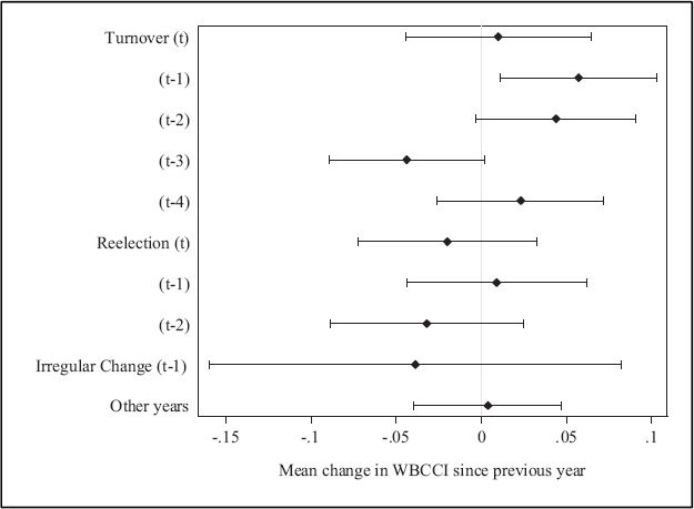
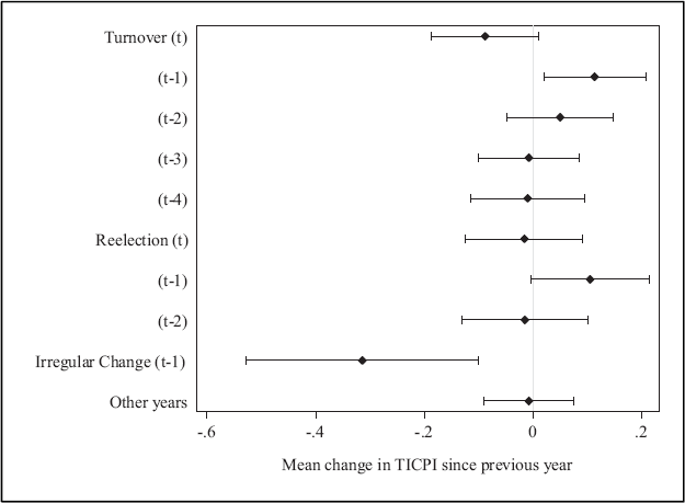
The trend is illustrated by Figure 1 and Figure 2, which show the results of an ordinary least squares (OLS) regression of ΔY1 on several dummy variables for the WBCCI and TICPI, respectively. The dummies differ according to the number of years that have passed since a particular event. For example, Turnover(t) equals one if the observation (country-year) included a turnover election, while Turnover(t-1) equals one if the observation is one year after a turnover election (for the same country). The regressions exclude a constant term and include instead a dummy variable for excluded category years. Thus, each coefficient estimate is the mean for a group of observations, and the confidence intervals indicate how those changes compare to zero. At the bottom of each figure, the excluded group (“Other years”) is shown to have a mean change that is close to zero. By contrast, Turnover(t-1) years exhibit a mean change that is both statistically positive and larger than the change of any other group – that is, the indices show unusually large increases in the years that immediately follow turnover elections.
These tests exclude Irregular Change(t-1)=1 observations.
One-Year WBCCI Changes (Post-2002) Regressed on Nine Year Indicators
One-Year TICPI Changes Regressed on Nine Year Indicators
Figures 1 and 2 show several other patterns. First, mean WBCCI change in Reelection(t-1) years is zero, as H2 anticipates; however, mean TICPI change in Reelection(t-1) years is markedly positive. Second, the coefficient on Turnover(t-2) is positive in both figures, suggesting that many countries exhibit two consecutive years of index gains after turnover. Third, Figure 1 shows evidence of a postsurge decline in corruption perceptions: in Turnover(t-3) years the ΔY1 is negative and of such magnitude as to erase the improvement that comes in the previous year. With the TICPI, however, there is no clear indication of a postsurge decline – except perhaps in turnover election years, which raises the possibility that the increase in Turnover(t-1) years is not something unusual but instead a more routine regression to the mean. While this paper's theory would predict some mean regression – because worsening corruption perceptions before an election can contribute to turnover – it begs the question of whether the ΔY1<0 in Turnover(t) years should be emphasized instead of the ΔY1>0 in Turnover(t-1) years. This question is answered in the next subsection, where the regression includes a lagged dependent variable.
Finally, Figure 2 shows that the TICPI decreases after irregular transfers of power, while Figure 1 shows that the effect of irregular transfers on the WBCCI is mixed. Either result might have been expected. While a coup or unexpected resignation may often heighten political anxieties and thus prompt perceptions downgrades, it can also be taken to signal the end of a troublesome period.
While Figure 1 and Figure 2 provide some indication of how index changes following turnover elections compare with index changes in other years, the comparison can be improved by adding control variables and accounting for serial correlation. Equation (1) includes a lagged dependent variable as well as control variables (Xj) and is estimated with OLS with panel-corrected standard errors (OLS-PCSE) to account for serial correlation (see Beck and Katz 1995):

Coefficients β2 and β3 estimate how index changes in the years that follow turnover elections and reelections compare with index changes that occur in other years. If mean change in excluded category years is zero, then H1 and H2 predict β2>0 and β3=0, respectively. The model does not provide a clear test of the “decline” part of H1; that is tested with a different model below.
It is reasonable to expect a negative coefficient on the lag (β1<0) because of regression to the mean. 18 Figures 1 and 2, however, suggested that index changes following turnover elections are often positive for two consecutive years, which would decrease the chance of β1<0. This is not a concern, but it does mean that the model could be improved by including a Turnover(t-2) dummy to account for how those years differ from other years. 19 If it is common to observe index gains in both the first and second years after a turnover election and if it is otherwise atypical to observe back-to-back years of a ΔY1>0, Turnover(t-2) will receive a positive estimate and its inclusion will make the coefficient on the lag more negative.
Few countries exhibit a clear long-term trend in either index. The closest instance would be Uruguay's TICPI, which increased in eight of eleven years.
As explained, the inclusion of Turnover(t-2) is not to “control” for countries that experienced turnover in back-to-back years. No country had such an experience.
Control variables include Irregular Changei(t-1), ALBAi(t-1), and the following:
20
the (mean-centered) percent change in real GDP per capita since the previous year. This variable is likely to receive a positive coefficient estimate, indicating that economic growth is correlated with less perceived corruption. =1 if a major corruption scandal implicating the executive branch broke during the year; =0 otherwise. This variable is meant to account for scandals that have the potential to significantly alter corruption perceptions. It therefore ignores “minor” scandals or scandals in countries already perceived to be highly corrupt and only accounts for scandals that are particularly egregious or highly unusual for the country in which it occurs. Because there is no simple way to operationalize this variable for all Latin American countries over 15 years, the coding is impressionistic. Four cases are deemed sufficiently important to be coded Scandalit=1: the 2004 corruption allegations that implicated former presidents Rodríguez and Calderón in Costa Rica; the MOP-GATE and Caso Coimas scandals that implicated Chile's government in 2002; the bribery revelations in Peru 2000 that prompted Alberto Fujimori's resignation; and the mensalão in Brazil 2005 – a corruption scandal that was attention-grabbing even by Brazilian standards.
21
Of course, one could make a case to exclude one of these scandals or to include other scandals, but wrestling with various coding schemes for this type of control variable is not worthwhile in this context, as there are no strong reasons to suspect that any coding scheme will dramatically alter how the key variables of interest (i.e., Turnover and Reelection) behave in the statistical model. Scandal is expected to receive a negative coefficient estimate. =1 if the government nationalized a sector of the hydrocarbon industry; =0 otherwise. Nationalization=1 for Argentina 2004, Bolivia 2006, Ecuador 2006, and Venezuela 2001. The variable serves as an additional measure of “leftward” policy change, at least among countries that have significant hydrocarbon resources to nationalize. It is included because nationalizations, even when partial, receive considerable attention at home and abroad. If corruption perceptions indices are heavily influenced by risk consultants and other foreign analysts, the variable is likely to receive a negative estimate.
Other variables that were analyzed include whether the president was elected nonconsecutively, whether there was reported fraud or violence surrounding the election, and whether the country signed or implemented a trade agreement with the United States. None of these variables affected the results.
The mensalão, or “big monthly stipend,” was furnished to lawmakers so that they would support the government's agenda.
Table 2 reports OLS-PCSE estimates of (1). The first two regressions use the post-2002 WBCCI; the second two, the TICPI. 22 The results of the first and third regressions indicate that Turnover(t-1) years exhibit a statistically positive ΔY1 relative to excluded years (p<.10 in both regressions) and that Reelection(t-1) years do not. Because the model includes a lagged dependent variable, we can conclude that the increase in Turnover(t-1) years is not simply regression to the mean. Regressions two and four add Turnover(t-2) to the model. As expected, the variable receives a positive estimate and makes the coefficient on the lagged dependent variable more negative. Also, the predicted changes in Turnover(t-2) years, after taking into account the increase in Turnover(t-1) years and the coefficient on the lag, are .04 (WBCCI) and .025 (TICPI). This suggests again that most countries experience two years of index gains after turnover.
Coding of Presidential Election Variables, 1996–2010
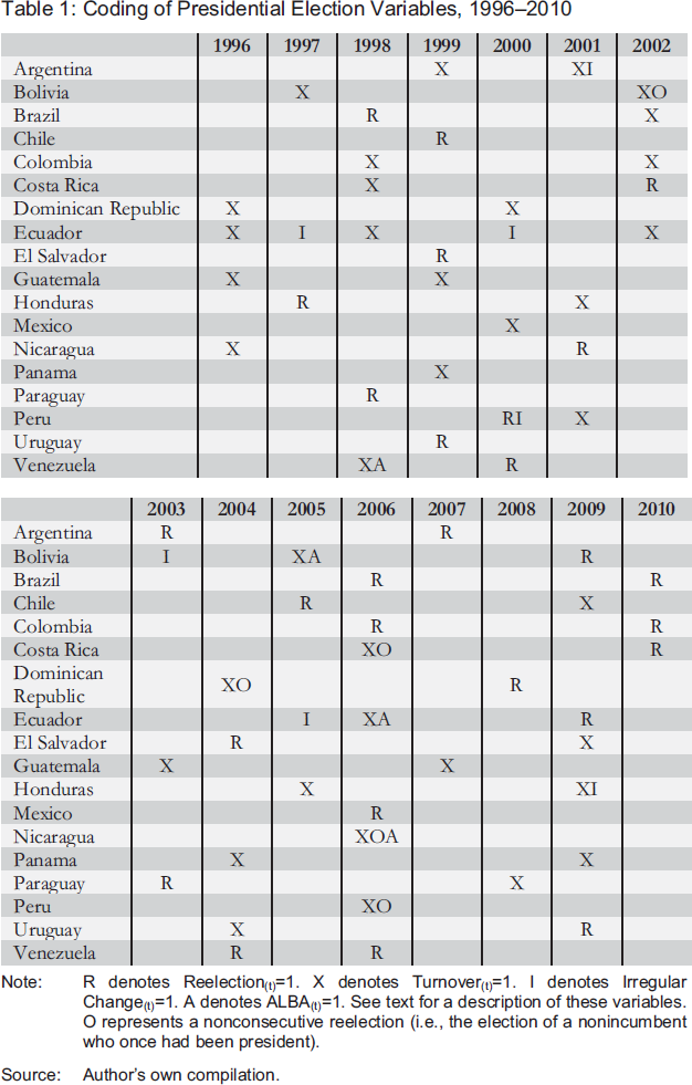
Note: R denotes Reelection(t)=1. X denotes Turnover(t)=1. I denotes Irregular Change(t)=1. A denotes ALBA(t)=1. See text for a description of these variables. O represents a nonconsecutive reelection (i.e., the election of a nonincumbent who once had been president).
Source: Author's own compilation.
Estimates were obtained with the xtpcse command in Stata 12.
Unlike with turnover elections, significant changes in the corruption indices do not follow hydrocarbon nationalizations. Also, the turnover surge is not significantly lower for those presidents who joined ALBA. Note also that the estimates on GDP Growth Rate and Scandal are always in the anticipated direction, and that the latter is significant with the TICPI.
The analysis has shown that the average turnover election is followed by one-year increase of roughly .06 WBCCI units and .1 TICPI units. These changes are not large, with each being about one-twentieth of the standard deviation in the global index. A turnover election does not make Nicaragua look like Costa Rica or Argentina like Chile. Still, the change is large enough to move most countries up a spot in the ranking of Latin American states. 23
In the post-2002 data, .06 WBCCI units is sufficient to move 67 percent of countries up a rank, while .1 TICPI units would move 69 percent of countries up a rank.
Of course, some increases are larger than average, while others are smaller (see Table 3). Thus, we might ask how common it is for a turnover election to be followed by a “large” increase. If (say) a large increase exceeds .15 WBCCI units or .3 TICPI units, then the answer is 25 percent and 20 percent of the time, respectively. These frequencies are twice what are observed in the dataset, as only 12.5 percent of WBCCI changes and 9.8 percent of TICPI changes are so large. Additionally, the correlation between a dummy variable that is unity for changes that exceed these thresholds and Turnover(t-1) is significant with both indices (WBCCI: p<.07, N=144; TICPI: p<.05, N=215). There is thus a disproportionate chance of observing large index gains in Turnover(t-1) years.
One-Year Changes in Corruption Perceptions Indices, OLS-PCSE Estimates
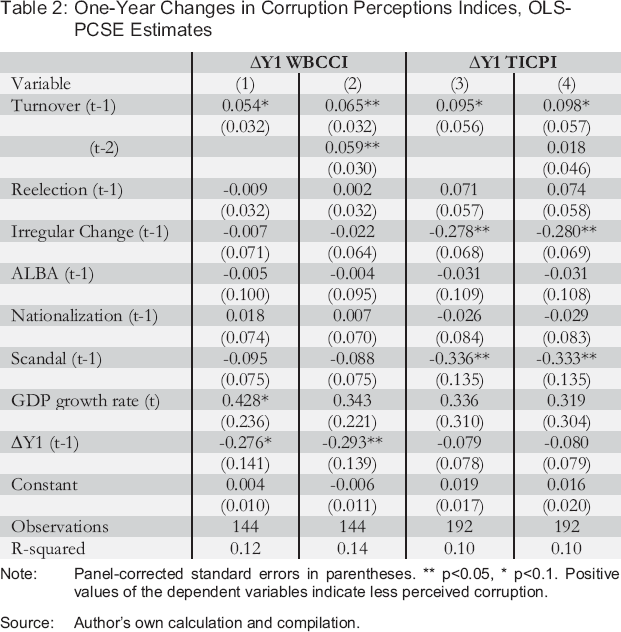
Note: Panel-corrected standard errors in parentheses.
p<0.05,
p<0.1. Positive values of the dependent variables indicate less perceived corruption.
Source: Author's own calculation and compilation.
At the same time, large gains are not likely to follow reelections. While five Turnover(t-1) observations have a ΔY1>.15 WBCCI units, that occurs after only one reelection – Bolivia 2009. Similarly, eight elections are followed by TICPI gains of .4 or more, but only two are reelections, and one of those (Chile 2000) could arguably have been coded as a turnover election. 24
The other instance is Paraguay 1999.
The examination of two-year changes permits use of the pre-2002 WBCCI, allows a test of whether the two-year surge is statistically significant, and allows a reasonable test of the “decline” portion of H1. Because H1 does not predict an exact timing of the postsurge decline – its starting year can vary – it would be overly restrictive to test for it in any particular year. This section studies the size and frequency of index declines during the second two-year period after turnover elections. 25
Of course, the second two-year period may not capture all “declines.” Mexico 2000–2006 is an example. After Fox's election, both indices increased over Y12 and both ended the six-year term about where they started in 2000. However, only the WBCCI declined during Y34. The TICPI declined during Y56.
Table 3 lists the first four years of index changes that followed turnover elections, excluding those that immediately followed or preceded an irregular change. It shows that most countries’ scores increased over the first two years (Y12) (though some of the gains were larger after only one year) and that many of the improvements decreased over years three and four (Y34). With regard to turnover elections before 2009, 73 percent (WBCCI) and 67 percent (TICPI) saw a ΔY12>0. Of those that occurred before 2007 and had a ΔY12>0, 67 percent (WBCCI) and 40 percent (TIPCI) saw a ΔY34<0.
These figures do not account for other determinants of index change, and it is clear from Table 3 that economic conditions matter considerably. In particular, countries that experienced either rapid economic growth during Y34 (second-to-last column) or a marked acceleration in the growth rate from Y12 to Y34 (final column) were less likely to see a ΔY34<0. Indeed, the Pearson correlation (r) between Y34 index changes and growth rates is .61 when using the WBCCI (p<.01, N=20) and .51 when using the TICPI (p<.02, N=18). 26 Interestingly, the opposite relationship is observed during Y12, when r=-.41 with the WBCCI and r=-.31 with the TICPI. This may occur because worse economic conditions at the time of the turnover election solicit greater relief with the change of administration. Regardless, it is unsurprising that the index-economic growth relationship is more strongly positive during Y34. A poorly performing economy is less likely to damage perceptions of governmental performance when the government is brand new than when the government has been in office for a few years. Anyway, the empirical connection between index changes and growth rates during Y34 implies that the entries that are most informative about postsurge declines are in the middle of Table 3 – that is, they are administrations that did not experience either rapid economic growth or an economic contraction during Y34. Tellingly, these cases were exceedingly likely to exhibit index downgrades during Y34.
These relationships are much stronger than those with annual change data; in other words, when examined over longer periods of time, corruption indices are more strongly related to economic growth rates.
To provide a statistical assessment of the two-year surge and two-year decline while controlling for economic conditions and other variables, I use OLS-PCSE and a model similar to (1) but which focuses on two-year index changes, ΔY2it = indexit – indexi(t-2). The regressions compare only a few types of observations: (a) those that are two years after an election (turnover or reelection), excluding those that are one year after either an irregular transfer or another election, and (b) those that are four years after a turnover election, excluding those that are three or fewer years after an irregular transfer or another election. As before, the syntax refers to these the other way around, as Turnover(t-2)=1, Reelection(t-2)=1, or Turnover(t-4)=1. The restriction to only these observations ensures the model is unencumbered by observations that straddle elections or that cover overlapping two-year periods. 27
The restriction makes for an unbalanced WBCCI panel. (The TICPI panel was already unbalanced due to “missing” data.) The regressions in Table 4 use the “pairwise” option in Stata's xtpcse, which allows estimation of the interpanel covariance matrix to be based on the years that are common to any two panels, rather than the years that are common to all panels.
A dummy variable for each group is included in each regression, and each regression excludes a constant term. Therefore, each coefficient compares a group mean to zero rather than to an excluded category of observations. The model also includes (i) a two-year lag of the dependent variable (Δ2yi(t-2)), (ii) the Two-Year GDP Growth Rateit, which is the mean-centered change in real GDP per capita over the previous two years, (iii) this last variable interacted with Turnover(t-4), which allows the model to account for differing relationships between index change and GDP growth throughout the electoral cycle, and (iv) Irregular Change(t-2).
The regression results are provided in Table 4. The first WBCCI estimates (regression one) are consistent with H1: there is a positive estimate on Turnover(t-2) and a negative estimate on both Turnover(t-4) and the lagged dependent variable. Both dummies are statistically significant, and a joint test of them with the lagged dependent variable shows all three to be highly significant (p<.001 in the χ 2 at the bottom of the table). 28 The estimates suggest that at mean levels of GDP growth, the average turnover election is followed by a .09 unit increase over Y12 and a .06 unit reversal over Y34.
Index Changes Following Turnover Elections
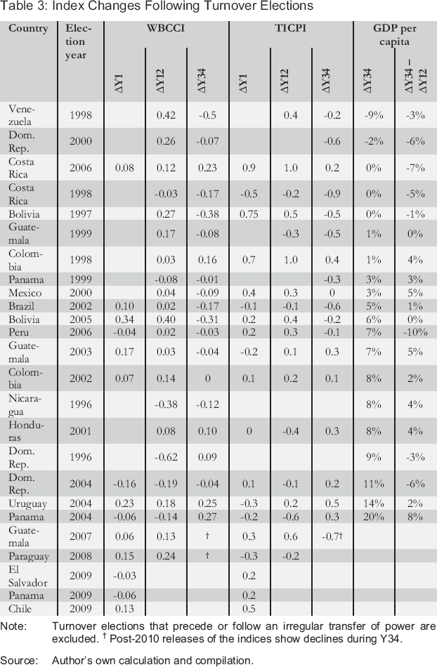
Note: Turnover elections that precede or follow an irregular transfer of power are excluded.
Post-2010 releases of the indices show declines during Y34.
Source: Author's own calculation and compilation.
After xtpcse, a test of multiple coefficient estimates is given by a chi-squared statistic.
The second regression includes Two-Year Scandalit, a dummy that is unity if Scandal(t-1)=1 or Scandal(t-2)=1. The variable is excluded from the first regression because this paper's theory anticipates its collinearity with Turnover(t-4) – that is, if one of the reasons for the decline is the increased frequency of high-level corruption scandals, then the statistical model does not require both Turnover(t-4) and Two-Year Scandalit. The way that the results change in regression three conforms with this line of thinking, as the scandal variable causes the estimate on Turnover(t-4) to move toward zero.
Regression three indicates that at mean levels of GDP growth the average TICPI increase over Y12 is .17 units and the decline over Y34 is one-third as large. About two-thirds of the decline is attributed to the Turnover(t-4) coefficient; the remaining third, to the lagged dependent variable. Although neither estimate is statistically significant, a joint test of them plus Turnover(t-2) rejects the null hypothesis. As with the WBCCI, the addition of the scandal variable causes the Turnover(t-4) coefficient to move toward zero (regression four), which suggests anew that the decline is partly due to corruption scandals. In short, all four regressions in Table 4 provide evidence of a surge-and-decline pattern. The data also support H2, as not one regression suggests a significant reelection effect.
Two-Year Changes in Corruption Perceptions Indices, OLS-PCSE Estimates
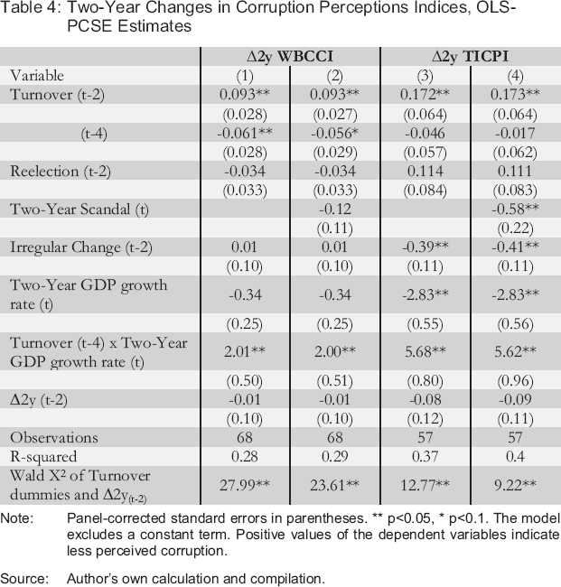
Note: Panel-corrected standard errors in parentheses.
p<0.05,
p<0.1.
The model excludes a constant term. Positive values of the dependent variables indicate less perceived corruption.
Source: Author's own calculation and compilation.
Lastly, I illustrate the results of regressions that are similar to those in columns one and three of Table 4 except for their inclusion of Reelection(t-4) observations and their exclusion of observations not in four-year terms. 29 Because this model is unencumbered by terms of varying length, it facilitates plots of predicted index changes over whole presidential terms. Holding GDP change at its mean and setting the lagged dependent variable to zero for the first two-year period, Figure 3 provides this plot for the WBCCI. 30 The figure shows that the average two-year surge is roughly one-tenth of the standard deviation in the global index and that it declines by about one-third over Y34. The pattern repeats if the president loses his reelection bid and a new government is installed. 31 If the government wins reelection, however, the WBCCI decreases over each of the next two-year periods to the point that the predicted change at the end of the term is close to where it was eight years before. The TICPI pattern is similar (Figure 4), the only differences being that the postsurge decline is less dramatic and that there is some improvement with reelections. Yet, the difference associated with a two-term president is about the same and much more modest than the change that accompanies a president's first two years in office.
The results are not shown for considerations of space; they are available from the author's website.
The figures exclude confidence intervals because post-xtpcse tests of multiple coefficients are provided by a chi-square statistic.
The second-term surge differs slightly because the lagged change is not zero.
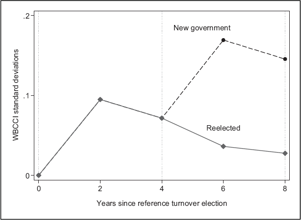
Predicted Change in WBCCI Following a Turnover Election
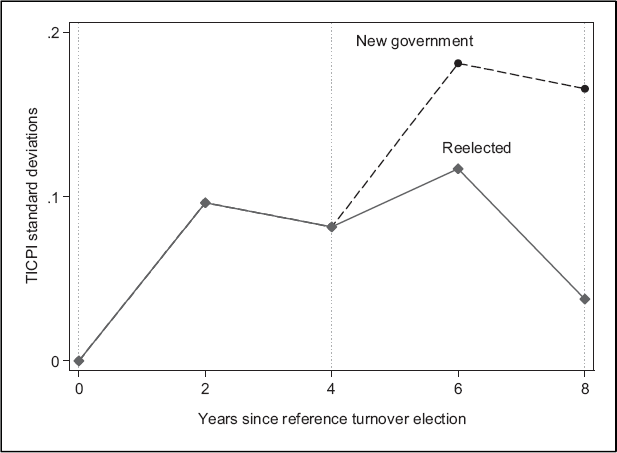
Predicted Change in TICPI Following a Turnover Election
The main conclusion of this study is that to understand perceptions of corruption in Latin American countries one must attend to the presidential election cycle and particularly the changes that follow turnover elections. However, the results and theory have other implications. For example, the temporary boost in perceived corruption control that follows partisan turnover in the executive branch will tend to strengthen public support for democratic institutions (see Canache and Allison 2005; Seligson 2006; Bohn 2012) as well as soften the demand for political reforms to counter corruption. The timing of the latter is important because it occurs when governments typically have the most political capital to spend on a reform effort. 32
The ebb and flow of corruption scandals and corruption perceptions may also matter for nonconcurrent elections, with those that occur shortly after turnover tending to be more favorable to the government than those that occur later. Cf. Shugart (1995).
Other implications depend on the specific reasons for perceptions change. I have argued that in any given case one or more of several mechanisms are responsible for the turnover surge. One is that turnover will tend to decrease political corruption whenever the outgoing government is unusually corrupt or wherever corruption tends to grow with government tenure. Separately, a public that is sanguine about a change of political leadership can overestimate the degree to which the new administration improves corruption control. The relative lack of high-level corruption scandals during the early stages of a new government is a third way that turnover can buoy perceptions of corruption control. Although this study does not test these mechanisms, it provides some evidence that high-level corruption scandals in Latin America have rarely occurred during a new government's first couple of years. Furthermore, its quantitative analysis suggests that scandals are at least part of the reason for the postsurge decline in perceived corruption control. Future research could seek to ascertain the relative contributions of scandals and presidential approval ratings to the surge and decline, though it will remain difficult to determine the degree to which high-level corruption varies and influences perceptions over such periods of time. Measuring corruption (rather than perceptions) is only part of the challenge; another is dealing with the issue of corruption affecting the other two explanatory variables (the likelihood of corruption scandals and public opinion about the government) (cf. Zechmeister and Zizumbo-Colunga 2013).
A priori, however, the turnover surge should be viewed as more rooted in perception than reality. This is not because there are not good reasons to think that political corruption might often decline (even if only temporarily) after an election has brought a partisan transfer of power. Rather, it is because the perceptions surge occurs precisely when public optimism is high and corruption scandals are few, and because there is already much evidence to suggest that corruption perceptions diverge from corruption realities (e.g., Morris 2008, 2009; Olken 2009). For the surge to reflect (rather than merely coincide with) a change in actual corruption, it must be the case that observers perceive that change and that their perceptions are little influenced by expectations or hopes that the new administration will resist and restrain corruption better than its predecessor. To the extent that this does occur, the perceptions surge documents the longevity of transition politics in presidential democracies, and the data would suggest that turnover results in cleaner politics for about two years. However, it is more likely that the importance of the perceptions surge lies in the realm of public opinion and the political consequences thereof.
The empirical findings of this paper have still broader relevance that stems from corruption perceptions indices being so widely used. A considerable amount of cross-national research on the causes and consequences of corruption employs these indices, and the results presented here suggest that in such applications it may be necessary to account for the regular fluctuations that appear after turnover elections. While this study cannot say whether turnover will have the same importance for index rankings in models that include parliamentary systems or nondemocracies (though that is a worthwhile avenue for future research), it demonstrates that turnover has an important effect on index values in Latin America.
The pattern also matters for organizations that utilize perceptions indices to gauge countries’ strides against corruption. This includes the Millennium Challenge Corporation (MCC), which allocates foreign aid according to how countries perform over time in the WBCCI (and other governance indicators). For instance, Honduras received a grant of USD 205 million from the MCC in 2004, not long after the turnover election of November 2001. The WBCCI was not compiled in 2001, but Honduras’ WBCCI increased markedly from 2002 to 2003. In fact, Honduras’ largest one-year improvement in the WBCCI for the period examined for this study was in 2003. That change may have accompanied real headway against corruption, and the turnover election may have contributed to such a development. However, the ability of turnover to independently improve corruption perceptions should be an important consideration for the MCC and other organizations that use perceptions indices to evaluate corruption control. Postturnover periods may demand special scrutiny to ensure that any index gains relate to significant developments in corruption control and not merely to public optimism about government turnover.
It similarly matters how indices are interpreted by the media, not least because it can influence diagnoses and reform agendas. It is also possible for foreign discourse about a country's index rank to influence domestic perceptions of corruption (Brinegar 2009). Of course, this study emphasizes the reverse process (i.e., that perceptions affect the indices), but feedback effects are possible. In any case, a worthwhile question for future research concerns the relative contributions of foreign and domestic perceptions to postturnover index change. Because the indices combine data from both types of audiences, we may suppose that events and trends that affect the indices do so via both audiences. However, the possibility remains that the turnover surge is driven predominantly by one audience or the other. Any such divergence would beg another question about which audience more accurately perceives the amount of corruption in a political system. The answer to that question would help us better understand the degree to which corruption perceptions reflect corruption realities.