Sage Journals: Discover world-class research

Abstract

The present study deals with the flames of ammonia–hydrogen blends that form a prospective fuel for power generation in practical devices. In particular, the spatial flame dynamics of the bluff body stabilized laminar and stratified ammonia–air/hydrogen–air mixtures with acoustic excitation are considered. For this, we consider a radially staged burner consisting of two concentric tubes namely, the inner and outer tubes with the bluff body housed by the former. Two annulus passages are formed between (i) the inner and outer tube, and (ii) the inner tube and bluff body in which premixed hydrogen–air and ammonia–air mixtures are supplied, respectively. The stratification is controlled by varying the upstream location of the inner tube about the burner exit, termed mixing length taking the values namely, 20 mm (stratified), 60 mm, and 100 mm (unstratified). Time-resolved images of the flames are obtained using OH* (320 ± 10 nm) and NH₂* (632 nm ± 10 nm) filters. For the unforced stratified flames, the flames are narrower and the spatial separation between OH* and NH₂* region increases towards rich NH₃/air mixtures (ϕ_NH3–air) compared to the unstratified flames. In addition, the mean spatial OH* is relatively localized for the unforced stratified flames. For any operating condition of the flames, the forced flame response is significant for frequencies < 120 Hz. The rich stratified flame exhibits a higher response at a frequency of ∼ 40 Hz compared to the unstratified flame having a flatter response. The forced flames accompany lobed spatial patterns in OH* and NH₂* for richer ϕ_NH3–air. The flame oscillation registers a non-sinusoidal oscillation for the rich stratified flame compared to flames of any other condition. The main effect of stratification is the alteration of flame shape resulting in a low-frequency response for which regions of significant flame flapping coincide with regions of peak flame OH*.

Keywords

Bluff-body stabilized flames radial staging ammonia–hydrogen blends flame response stratified flames and spatial flame dynamics

Introduction

Fossil fuels have virtually powered the entirety of the energy needs of humankind, both in the form of direct power generation and transport. The generation of carbon dioxide and water vapor as the most stable combustion products, with a focus on the former on heating the earth's atmosphere to above 1.5 °C above the pre-industrial age, has resulted in increased interest in carbon-free fuel-based combustion. Amongst such fuels, hydrogen is an attractive option for clean energy production. However, the density and high reactivity of hydrogen have posed concerns regarding safety and the required infrastructure to utilize hydrogen in its pure form. These opportunities and challenges have led to studies on the potential of one of the most successful commercial products namely ammonia as a way towards zero-carbon fuels.

Ammonia is an excellent hydrogen carrier with higher hydrogen density than liquefied hydrogen and is much cheaper to produce and store.^1,2 The primary issue with ammonia combustion is its low calorific value, a narrower range of flammability limit, and high auto-ignition point, which translates to low flame speed (∼5–7 cm/s at STP). This poses a significant challenge in gas turbines requiring significant modification to flame holder design to ensure flame stability. Also, NOx emissions, primarily comprising NO² are significantly higher compared to methane combustion, especially in lean flames, which becomes insignificant towards the equivalence ratio of ∼1.2, due to NOx reduction by ammonia. This implies that ammonia as a stand-alone fuel primarily needs to be burnt at richer conditions for low NOx emissions.

The challenges of burning pure ammonia and the operating equivalence ratio restricted by the low NOx emissions warrant the need for specific combustion technologies and operating conditions. For instance, Li et al.³ in their numerical simulations have shown an improvement in ammonia combustion when the oxygen concentration increased from 21% to 30% with reductions in NOx in rich conditions. Increasing the O₂ content by 9%, the laminar flame speed of NH₃ is found to increase by a factor of 2.8 as shown by Shrestha et al.⁴ in the experiments conducted in a constant volume chamber. The strategy of preheating ammonia to a range of temperatures by Chen et al.^5,6 improves the combustion characteristics of non-premixed ammonia flames along with a reduction in NOx emissions. The preheated NH₃ flame structure exhibited a blue flame base and a blue outer shell encompassing yellow regions compared to non-preheated ones, which comprise dominant yellow flames.

Typically, rich ammonia combustion is associated with the cracking of NH₃ resulting in the generation of H₂ which undergoes combustion subsequently leading to an inherent staged combustion.² Another form of staging is splitting both fuel and air between primary and secondary regions, with the latter being similar to the rich-burn quick-quench lean-burn (RQL) concept. Pugh et al.⁷ in a swirl combustor have adopted the RQL concept and have shown the low NOx operation of the combustor for the premixed and diffusion flame to occur in the rich and global lean operating equivalence ratios, respectively. A lean-lean staging through 8% NH₃ fuel split into the secondary combustion zone is found to promote around 80% reduction in NOx along with an increase in the flammability limits in a swirl configuration used by Lee et al..⁸ The numerical simulation of two-stage ammonia combustion in a constant-pressure sequential combustor by Heggset et al.⁹ emphasizes the low NOx benefits of staging. In the case of the pressure effect, Okafor et al.¹⁰ have shown that the NOx reduces with an increase in the ambient pressure in premixed flames.

For increased flexibility in ammonia combustion, it is better to resort to dual component fuel such as blending with H₂, which caters to carbon-free fuels and reduces the dependence on pure H₂. Typically, the addition of hydrogen overcomes the constraint of low reactivity of NH₃ and enhances its combustion. Studies in the constant volume chamber^11,12 and model gas turbine combustor^13,14 have shown an improvement in flame speed and an increase in the flammability range with an increase in H₂ volume fraction. The effect of H₂ addition is found to have the same effect as that of increasing the oxidizer.⁴ The addition of H₂ to NH₃ helps in operating the combustor in a fuel-flexible manner as shown by Ånestad et al.¹⁵ in their staged combustion study. In the lean operation, thermal NOx potentially increases,¹⁶ however, altering the volumetric ratio of NH₃ and H₂¹⁷ can be of benefit to reducing the emissions.

A prospective methodology to reduce NOx while ensuring flame stability would then be to use a stratified mixture of hydrogen and ammonia. This aspect is considered in the studies of Mashruk et al.¹⁸ and Jin and Kim¹⁹ in a lab-scale combustor to show a reduction in NOx with the stratification through the staging of H₂–air mixtures. The present investigation intends to deliberate on this specific aspect of hydrogen-blended ammonia–air mixtures to explore the impact of stratification on flame dynamics. As with any flame, it is imperative to obtain the flame behavior to the imposed acoustic oscillations to understand its dynamics, which is the main goal of the present study.

Generally, flames are receptive to acoustic perturbations while, at the same time, they are an acoustic source.²⁰ Under certain conditions, the acoustic feedback and the flame response interfere constructively leading to combustion instability. Typically, the flames involved in these phenomena are compact relative to the acoustic wavelengths. The characteristic features such as oscillation frequencies, damping rates, and mode shapes are computed from an eigenvalue problem in the context of a thermoacoustic model.^21,22 In this formulation, the flame response is represented through a flame transfer function, which relates the fluctuations in the heat release rate to those in the upstream velocity as a function of frequency.²³

Flame transfer functions can be determined experimentally by imposing velocity fluctuations and estimating the resulting heat release rate oscillations through flame radical emissions.^23–25 The dynamics of flame at a higher gain is related to the large-scale modulation of the flame.²⁴ Typically, the flame response is governed by the mean flame shape determined by burner geometry and operating conditions. For instance, in the studies of Kim et al.,²⁵ H₂ enrichment of CH₄ flames resulted in M-shaped flames that dampened the flame response compared to the V-flames. Similarly, the flame height modification due to different fuels resulted in different flame responses without changes in the mechanism controlling the flame dynamics.^26,27 In the case of burner geometry, Gatti et al.²⁸ have compared the transfer function of swirl, bluff body, and swirl-bluff body-dump configurations. They have reported modification of the mechanism of flame dynamics depending on the flame stabilization. As we can see the flame shape and hence the flame response, is dictated by the distribution of spatial heat release rates, which will be considered in this investigation. This aspect in particular is important as the H₂ blending to NH₃ would alter the flame shapes and its response.

Recently, the emerging interest in carbon-free fuel has prompted in few studies in the direction of flame dynamics. The flame response for premixed ammonia–hydrogen blends in a premixed burner has been investigated by Wiseman et al.²⁹ in which the flame response is found to have a higher response in the lower frequency compared to methane flame but with increased cut-off frequency. In a modeling study by Nunes and Morgans,³⁰ the flame response is found to increase with an increase in the H₂ promoted by increased flame speed. Compared to premixed flames, a stratified dual-fuel mixture opens the possibility of tailoring the flame response to a significant extent, to decrease the susceptibility to combustion instabilities. In the control of such high amplitudes, stratification through the radial staging of H₂–air has been reported to reduce self-excited thermoacoustic instabilities in a swirl combustor considered by Katoch et al..³¹ Another study, Lee et al.¹⁹ have reported a reduction in the flame response in a radially staged NH₃/H₂ combustor. They attribute this to the interaction of slow-burning NH₃–air and fast-burning H₂–air flames that prevent the formation of organized structures. These observations make stratified flames relevant to practical systems in terms of flame dynamics, stability, and reduced emissions. Hence it is important to understand and characterize their dynamics in a simplified experimental system, which is a key aspect of this current investigation.

In this study, we consider ammonia–hydrogen flames of different stratifications, stabilized on a bluff body and subjected to external acoustic excitation in a laminar flow condition. In this configuration we employ a radial stratification similar to that used by Jin and Kim¹⁹ and Katoch et al.³¹, but with a key difference is that the degree of stratification, a key control parameter can be varied in a laminar flow condition to tailor the NH₃–H₂ mixtures that modify the flame response. The main objective of the present work is to study the effect of the mixture tailoring on (i) the mean flame shape and (ii) spatial flame dynamics. We explore the relation between the spatial flame dynamics and the mean flame shape. For this, we resort to mapping active regions of flame fluctuations using OH* and NH₂*, for lean and rich NH₃–air mixtures, forcing frequencies, and stratification.

Experimental setup and operating conditions

The experimental setup employed is a radially staged bluff body burner as shown in Figure 1. The rig consists of concentric tubes of diameter d_i= 14 mm and d_o= 19 mm labeled as the inner and outer tubes, respectively. The outer tube is mounted on a reducer that is subsequently fastened to the settling chamber of inner diameter 100 mm fixed to the bottom plate. Similarly, the inner tube is fixed to a reducer unit fastened to the bottom plate. In addition, inset tubes of lengths L_IT= 40 and 80 mm are added between the reducer and the inner tube. This results in a retraction of the inner tube with respect to the burner exit and the retraction length is termed as the mixing length denoted by L_m. In this study, the mixing lengths of 20 mm, (L_IT= 80 mm), 60 mm (L_IT= 40 mm), and 100 (L_IT= 0 mm) are considered.

Figure 1.

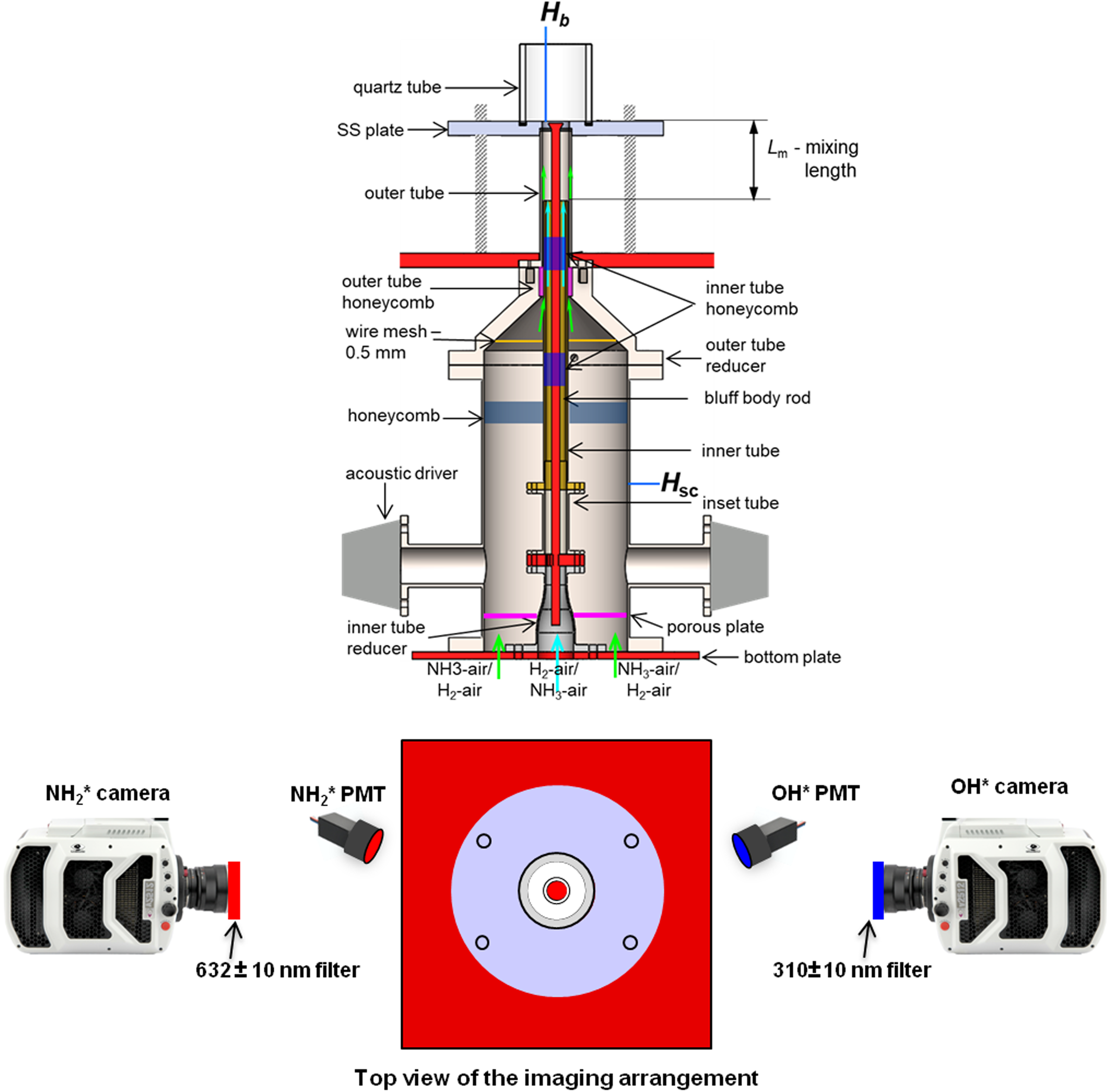
Experimental setup with labeled parts along with a top view of the camera and PMT arrangement. H_sc and H_b denoting the HWA at the settling chamber and burner exit, respectively.

The bluff body unit consists of a long rod of length 300 mm and 6 mm diameter that expands to d = 11 mm over a length of 4.5 mm resulting in a conical bluff body. The bottom region of the bluff-body rod is threaded and fastened to a flange that is sandwiched between the inset tube and the inner tube reducer as shown in Figure 1. In this configuration, the inner tube houses the bluff body. In sum, the overall assembly results in two annular regions, (i) between the inner and the outer tube termed as outer annulus (A1), and (ii) between the inner tube and the bluff body termed as inner annulus (A2) through which the reactants are supplied. The bottom plate carries (i) a pair of cylindrical blocks with orifices of diameter 1.5 mm to supply the reactants to the A1 region (ii) a flow adapter at its center to issue the reactant to the A2 region as indicated by the arrows as shown in Figure 1. The bottom plate is eventually mounted on a rigid table.

The settling chamber houses a porous plate of 2 mm diameter holes located 20 mm above the cylindrical blocks. This is followed by a honeycomb of 1.5 mm cell size with a wall thickness of 0.1 mm, followed by a wire mesh of size 0.5 mm fixed in the outer reducer section. Another honeycomb of cell size 1 mm is placed in the slot in the reducer section for flow passage A1 as marked in the figure. This honeycomb helps to center the inner tube with respect to the outer tube. For the inner tube, two honeycombs of 1 mm cell size and wire meshes of 0.5 mm holes are used in the A2 region, which serves to laminarize the approach flow and center the inner tube-bluff body assembly. The settling chamber has provision for installing acoustic drivers for the flame forcing tests. A 10-mm thick stainless steel plate is mounted atop the outer tube on which a quartz tube of inner diameter 44 mm and thickness of 5 mm is placed forming a region of sudden expansion. The test flames typically stabilize on the bluff body and extend downstream into the region of sudden expansion.

The reactants consist of streams of premixed H₂–air and NH₃–air mixtures issued into the annular passages A1 (outer annulus region) and A2 (inner annulus region), respectively, with an average flow velocity of 1.5 m/s. Air is issued using two mass flow controllers (MFCs) of range 0–50 SLPM, while for the H₂ and NH₃ gas, MFCs of flow rate range 0–10 SLPM are employed. The accuracy of all the MFCs is ± 1% of the full range. The approach flow is laminar with Reynolds number Re = 1300, estimated using the kinematic viscosity of 1.56 × 10⁻⁵ m²/s and the annulus gap of 13 mm formed by d_o= 19 mm and bluff body rod diameter of 6 mm upstream to the burner exit. Different flames are obtained by varying the NH₃–air equivalence ratio (ϕ_NH3–air) from 0.7 to 1.1 in steps of 0.2 for a constant H₂–air equivalence ratio (ϕ_H2–air) of 0.25. The test flames of L_m= 20 and 100 mm are termed stratified and unstratified flames, respectively, which will be used throughout the rest of the article. The test matrix consists of a total of six conditions with three ϕ_NH3–air and L_m cases. By varying L_m for a particular ϕ_NH3–air, we compare flames of the same thermal power for different stratification levels.

Measurement techniques

In the present study, one component hot-wire anemometer (HWA) (Dantec Dynamics, Model: 55P11) is mounted at the burner exit to (i) characterize the turbulence intensity of the non-reacting flow and (ii) calibrate the forcing system to obtain the desired velocity amplitude at the burner exit. For the forcing tests, a sub-woofer (Monacor-SPH135C) is fixed to the settling chamber; it is driven by an amplifier that is connected to a signal generator (Aim-TTi TGA1244). The input voltages to the amplifier for the forced tests are tuned to obtain a constant forcing intensity J = 4%, where J = uʹ/U_mean at the burner exit over a frequency range of 25–200 Hz. Additionally, another HWA is fixed in the settling chamber to monitor the velocity fluctuations during the non-reacting tests, which are used for tuning the forcing system in the flame tests. The tuning procedure is explained in the subsequent section.

The total intensity fluctuations of the flame radical emissions are acquired using two photo-multiplier tubes (PMTs), fitted with optical filters, 310 ± 10 nm for OH* (I*_OH) and 632 ± 10 nm for NH₂* (I*_NH2) intensities. The flame NH₂* and OH* are useful radicals to characterize the NH₃/H₂ flames.³² In addition, the spatial OH* and NH₂* chemiluminescence intensities are imaged using high-speed intensified cameras (Phantom V12). The cameras are controlled by a high-speed controller (LaVision system) and operated at 1000 frames/s for 2 s. The PMT and settling chamber HWA signals are sampled at 51.2 kHz for 2 s and digitized using a 24-bit NI-9234 DAQ during the flame tests. For the flame radical imaging, the field of view covers 100 mm in the streamwise direction (y) and 55 mm in the radial direction (r), covering 9d and 5d, respectively, with the origin considered at the bluff body center. The chemiluminescence images are acquired for a few forcing conditions.

Calibration procedure for the forcing tests

To excite the flame with a desired velocity fluctuation at the burner exit, the input voltages from the signal generator to the amplifier need to be calibrated for the frequency range of 25–200 Hz.

For the velocity measurements, two HWAs are used at (i) the burner exit (H_b), and (ii) the settling chamber (H_sc), as shown in Figure 1. For each frequency, the input voltage from the function generator (V_fg) to the amplifier is tuned to achieve J = 4% as measured by the top HWA using an iterative process. In this method, two guess values of the function generator voltage (V_fg) result in two J values, and the incurred error is used to update V_fg iteratively following the secant method to eventually obtain J = 4%. The corresponding HWA voltages in the settling chamber are noted for each forcing frequency as the algorithm iteration converges.

During the flame tests, since the HWA cannot be used at the burner exit, the settling chamber HWA voltage V_sc recorded for each forcing frequency in the non-reacting flow tests is used as a look-up table to auto-tune the function generator voltages. The auto-tuning algorithm does not always converge, resulting in the applied voltages to the speaker that yield velocity fluctuations deviating from the desired 4% intensity for a few frequencies. This is overcome by retuning the forcing system with different guesses to obtain the desired values at the burner exit.

Results and discussion

Unforced flow spectrum

Before we proceed to discuss the results of flame forcing tests, we show the baseline spectrum of the unforced flow oscillations, which is overlaid on the spectrum of one forced test case. The unforced streamwise velocity fluctuations are measured at the burner exit using HWA H_b and the estimated velocity intensity is ∼ 0.5%. The spectral content of the velocity fluctuations is obtained from the power spectral density (PSD) as shown in Figure 2.

Figure 2.

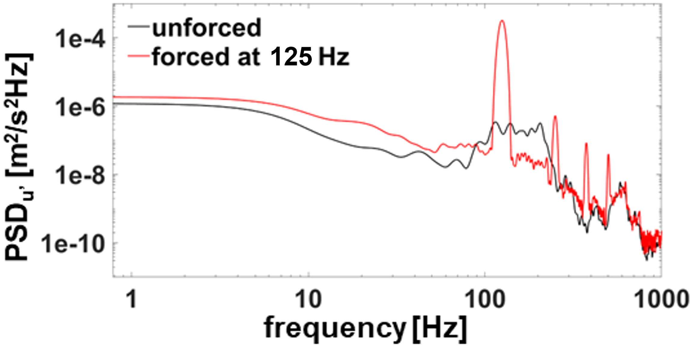
Power spectral density (PSD) of u' at the burner exit for forced and unforced conditions. (colour online).

The PSD shows a dominant band for the frequency range of 100–250 Hz and is broadband otherwise for the unforced flow condition. Despite the banded spectrum, its imprint on the flame is not significant as we did not observe oscillations of the unforced flames. For the forced flow, we consider the forcing frequency of 125 Hz. In this case, forcing results in an amplitude that is approximately three orders of magnitude stronger than that for the unforced case at the forcing frequency. This implies that the unforced flame oscillations would not affect the forced flame response. Here the chosen frequency is arbitrary, but the observed spectrum is similar to other forcing frequencies.

The flame response of forced flames

The flame oscillations are characterized using the flame OH* fluctuations that were employed in the previous investigation of the flame response in premixed²⁹ and stratified³¹ ammonia–hydrogen flames. The I*_OH oscillations of NH₃–H₂–air flames for any operating conditions are observed to be insignificant beyond 120 Hz, with significant responses in the range of 20–60 Hz for some cases. Such a lower frequency response is attributed to the longer time scale that is related to the lower flame speed of NH₃–air mixtures.³⁰

In Figure 3, we can observe that for any stratification, the lean flame has a relatively lower response compared to the rich flame over the tested frequency range. In the case of the unstratified flames, oscillations in I*_OH show a flatter behavior over the wide range of frequencies with a shallow peak around the frequency of 40–80 Hz. However, maintaining ϕ_NH3–air= 1.1, and decreasing the mixing length to L_m= 20 mm, the flame oscillations have a higher response for the lower frequency range. The highest fluctuation intensity is registered by the stratified flames of ϕ_NH3–air= 1.1 with a peak response around 40 Hz. This behavior is prevalent even for the stratified lean flames compared to the unstratified ones. A shift in the flame oscillation behavior from the unstratified to the stratified flame of the same power is attributed to the changes in the flame shape associated with spatial flame radical patterns.

Figure 3.

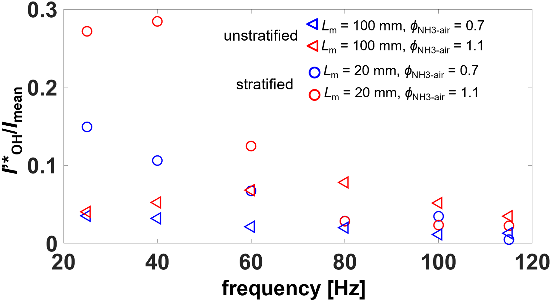
Normalized I*_OH fluctuation for various forcing frequencies and flame conditions. (colour online).

The complete picture of the flame response can be retrieved by flame forcing over a wider frequency range at a smaller frequency resolution. However, the present study being a preliminary one in the stratified NH₃–H₂ flames, we restrict to a few forcing frequencies mainly to focus on the spatial flame dynamics to imposed perturbations. In this regard, we discuss the time-averaged and the phase-averaged OH* and NH₂* fields for different flame conditions to highlight the effect of stratification and to point out the aspect that controls the flame response to different frequencies subsequently.

Flame visualization

Time-averaged unforced flames

The response of the flame to the external excitation depends on the baseline flame shape^25–28 and the spatial distribution of the flame radicals in the unforced conditions. Given this, we discuss the unforced flame shape for various conditions while emphasizing the effect of stratification. The time-resolved images of I*_OH and I*_NH2 fields are averaged and normalized using the maximum intensities. The average spatial I*_OH and I*_NH2 for L_m= 20 and 100 mm and for three conditions of ϕ_NH3–air are shown in Figure 4. For better visualization of the flame, the I*_OH and I*_NH2 are shown beside each other covering only half the flame. In addition, the flame length and flame cone angle at its base are computed in Table 1. For the estimation of flame properties from the image, we adopt the Otsu method of image binarization that employs a histogram-based standard method to determine a single threshold for the entire image. Following the binarization of the original image, flame edges are determined through the Canny edge detection method and subsequently the flame angle and the flame height are estimated.

Figure 4.

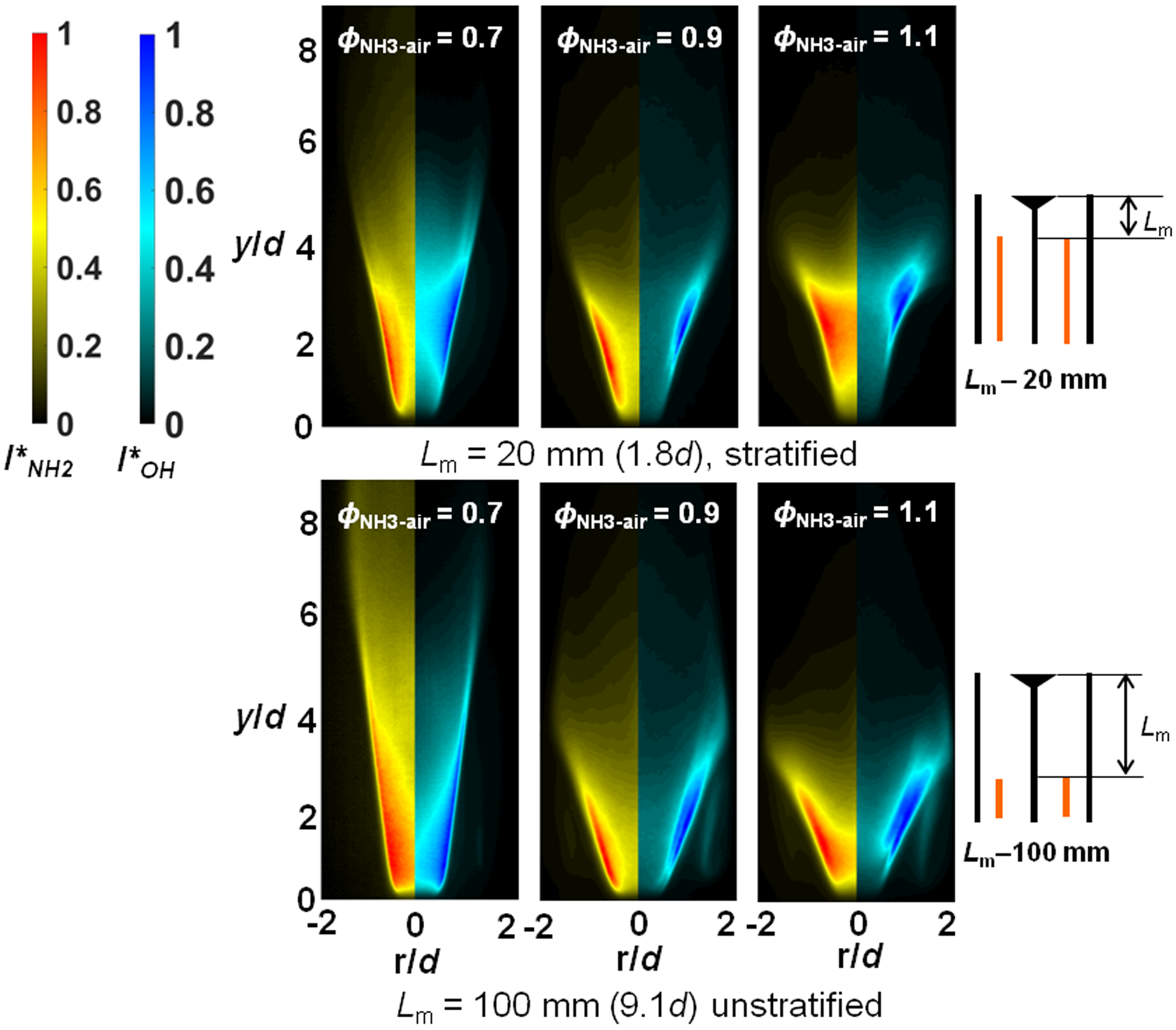
Time-averaged unforced I*_OH and I*_NH2 fields for L_m= 20 mm (top) and L_m= 100 mm (bottom). (colour online).

Table 1.

Flame length and angle for various operating conditions.

Flame angle (deg)		ϕ _NH3–air
Flame angle (deg)		0.7	0.9	1.1
L_m (mm)	100	7.5	17.9	24.0
L_m (mm)	20	12.1	16.4	17.6
Flame height (y/d)		ϕ _NH3–air
Flame height (y/d)		0.7	0.9	1.1
L_m (mm)	100	7.8	3.9	3.1
L_m (mm)	20	5.5	3.3	3.8

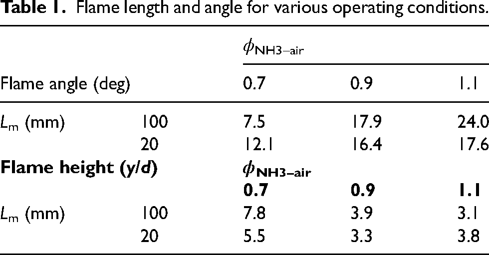
From the figure, for a particular L_m, the average flame cone angle at the flame base increases with an increase in ϕ_NH3–air, which is prominent for the unstratified flame. For the flames with an increased stratification, the average flame cone angle increases as ϕ_NH3–air increases to 0.9 from 0.7. However, increasing the ϕ_NH3–air to 1.1, the flame tends to be relatively more curved, deviating from a conical shape. The flame cone angle at its base reduces while increasing in the downstream location for ϕ_NH3–air= 1.1 compared to that for ϕ_NH3–air= 0.9. This behavior is attributed to the dominance of rich NH₃ combustion leading to a possible reduction in the flame speed arising from poor mixing with the H₂–air stream.

In the case of the stratification effect at a constant ϕ_NH3–air, the flame cone angle increases with an increase in L_m as shown in Table 1. Typically, at a constant L_m, an increase in ϕ_NH3–air results in an increase in the global flame speed of the mixture towards stoichiometric mixtures. However, at a constant ϕ_NH3–air, an increase in L_m leads to improved mixing between the H₂–air and NH₃–air streams before they approach the flame base. This in turn results in the better flammability promoted by the homogenization of H₂ in the overall reactant mixture thereby leading to an increase in the flame speed and hence the wider flame.

The disparity between the spatial dominance of OH* and NH₂* increases with an increase in both ϕ_NH3–air and L_m. Such an effect is more pronounced for the richer flame with the highest stratification. For instance, in the flame corresponding to L_m= 20 mm and ϕ_NH3–air= 1.1, the I*_OH is confined to region 2–4d from the bluff body as reflected by a sharper increase in its intensity. For the flames corresponding to L_m= 100 mm, the intensity variation is uniform from 0–3d in the streamwise direction over the entire flame length. In addition, the spatial disparity between OH* and NH₂* is observed to be insignificant compared to that in the stratified flames.

Typically, in the H₂–air flames, OH* is directly related to the heat release rates. In the NH₃ flames even though OH* was used as a marker to study the flame dynamics,^29,31 it can be contributed by both NH₃–air and H₂–air flames. But distinct markers for NH₃–air flames can be either NH*, NO*, or NH₂*. Of these NH₂* is the first intermediate that forms in the oxidation of NH₃ indicated by I*_NH2, while I*_OH would pertain to intermediates that lead to products.² Since I*_NH2 is associated with the commencement of NH₃ oxidation, it always precedes the I*_OH as was observed in premixed NH₃–air flames by Otomo et al..³³ The extent of disparity between I*_OH and I*_NH2 depends on the stratification. The observed spatial disparity for rich stratified flames can be attributed to NH₃ cracking resulting in NH₂* production and subsequent oxidation through OH* resembling staged combustion.^1,2 In unstratified flames, increased mixing promotes H₂ to enhance the NH₃ combustion leading to faster reaction and reduced spatial disparity between them.

In essence, the flame shape of the base state in the unforced conditions is determined by the operating condition, which would play a key role in shaping the flame dynamics in the presence of forcing as discussed subsequently.

Amplitude map of forced flames

In the following, the spatial dynamics of the forced flames are discussed using the amplitude maps for various frequencies and operating conditions. The amplitude map of I*_OH and I*_NH2 oscillations is formed by extracting the absolute values of their respective Fourier amplitudes at each spatial location. We consider the amplitude map for L_m= 20 and 100 mm and for ϕ_NH3–air= 0.7 and 1.1 as shown in Figure 5.

Figure 5.

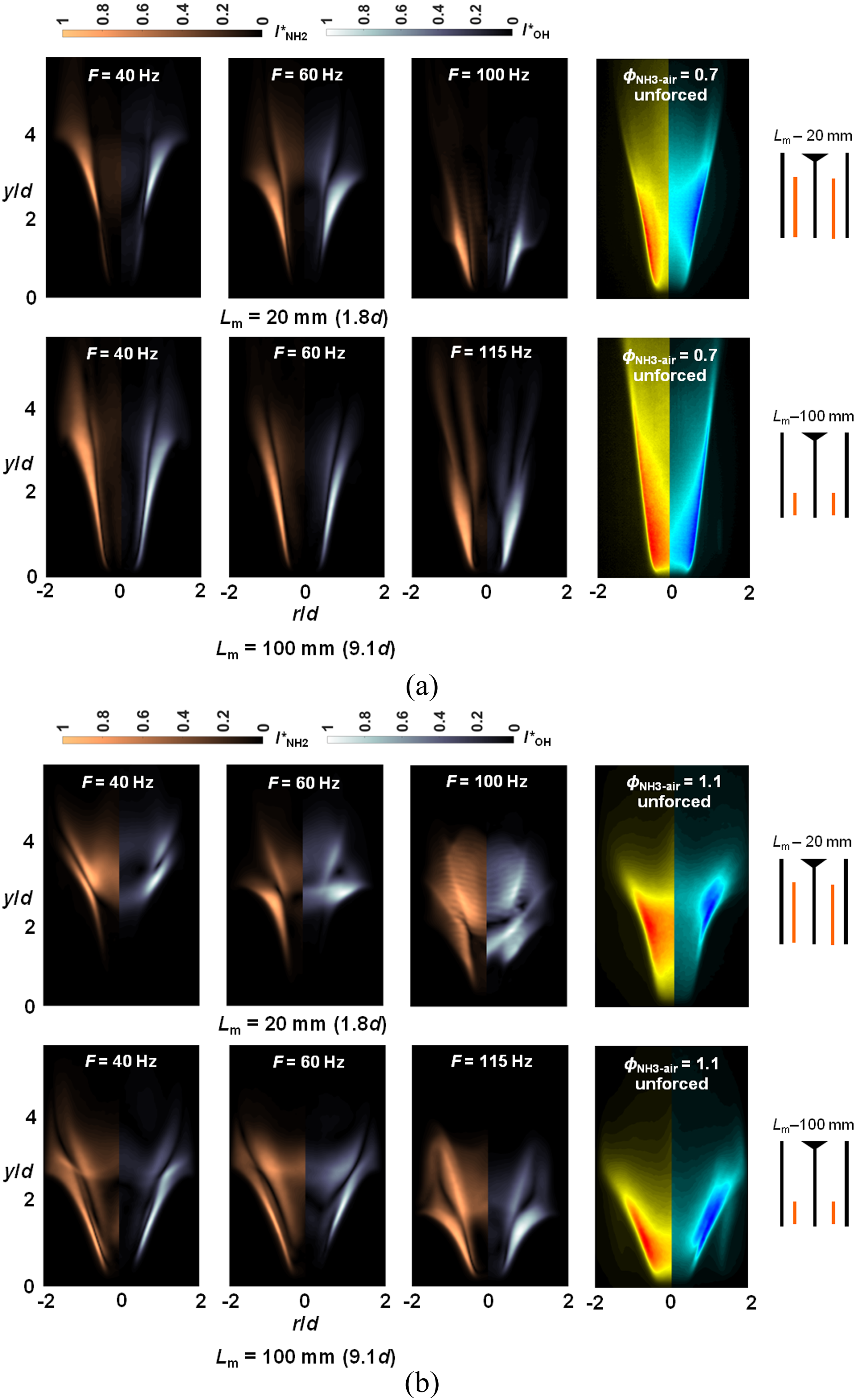
Amplitude map at different forcing frequencies for different test flames at (a) ϕ_NH3–air= 0.7, and ϕ_NH3–air= 1.1. (colour online).

The amplitudes are normalized with the maximum values to highlight all the features. We choose the mid-range frequencies namely, 40 Hz, and 60 Hz for both cases of stratified flames, while higher frequencies of 100 and 115 Hz are used for the stratified and unstratified flame, respectively, to discuss the amplitude maps. The amplitude maps are shown in Figure 5 for both OH* and NH₂* side by side along with the mean I*_OH and I*_NH2 to correlate the flame oscillations with the occurrence of peak flame regions.

From Figure 5(a), the regions of strong flame oscillations are prevalent around the flame boundaries compared to the inner regions for the lean flames of ϕ_NH3–air= 0.7 for both the mixing lengths and independent of forcing frequencies. The region of strong flame oscillations becomes prominent towards the flame base as the forcing frequency increases from 40 to 115 Hz due to the smaller length scale of the incipient flow structure with an increase in the forcing frequency. The flame oscillations of the unstratified lean flame (L_m= 100 mm) extend from the flame base to the downstream region. This is in contrast to the stratified flames wherein the peak oscillations occur only at downstream locations from the burner exit for 40 and 60 Hz. The extent of flame oscillation indicated by the brush thickness increases away from the burner exit. Such behavior is attributed to the increased flame flapping in the downstream locations caused by possible amplification of flame wrinkles/flow structures.³⁴

As the ϕ_NH3–air is increased to 1.1, the rich flames show a distinct feature compared to the lean flames shown in Figure 5(b). In this operating condition, the I*_OH and I*_NH2 fluctuations depict a prominent double lobe pattern for both L_m= 20 and 100 mm compared to leaner flame conditions. The double lobe pattern is relatively compact for the flames of L_m= 20 mm compared to that for the flames of L_m= 100 mm. The spatial extent of the lobe pattern correlates well with that of the mean spatial intensities of I*_OH and I*_NH2. The double lobe pattern could be attributed to the flame flapping due to the passage of wrinkles along the flame, which will be emphasized using the phase-averaged images subsequently.

One of the distinguishing features of the stratified flame is that its peak response is distributed over the region covering 2–4d compared to the flames having less stratification. Such a region could mark the recirculation zone length of the reacting flows in a sudden expansion configuration.^35,36

Typically, imposed velocity oscillations could result in flow structures along the outer shear layer of the sudden expansion. The length scale of the flow structure reduces with an increase in the forcing frequency. The observed upstream movement of peak flame fluctuations with an increase in the forcing frequency could be attributed to the reduction in the length scale. Further, for the highest flame response based on OH* as shown in Figure 3, the spatial extent of mean OH* distribution should be similar to the length scales of flow structures and flame oscillations.

We want to highlight that the mean flame OH* for L_m= 20 and 100 mm are most prevalent at around 2–4d, and 0–2d, respectively (Figure 4). This implies that the flames with higher stratification should have peak flame OH* responses towards lower frequencies compared to that for less stratified flames. The flame response behavior is controlled by the length scale of the vortices/wrinkles due to the excitation and its relationship with the key spatial flame radical distributions that govern the heat release rates.

Phase averaged NH₂* and OH* fields

Next, we present the flame dynamics through the phase-averaged intensity maps of NH₂* and OH* fields for different operating conditions and frequencies as shown in Figures 6 and 7. For the rich and lean flames of L_m= 20 mm, we consider the frequencies of 40 and 60 Hz, while for L_m= 100 mm flames, we examine the flame oscillations at 115 Hz. For the phase-averaged images, the phases of I*_OH fluctuations are used as a reference.

Figure 6.

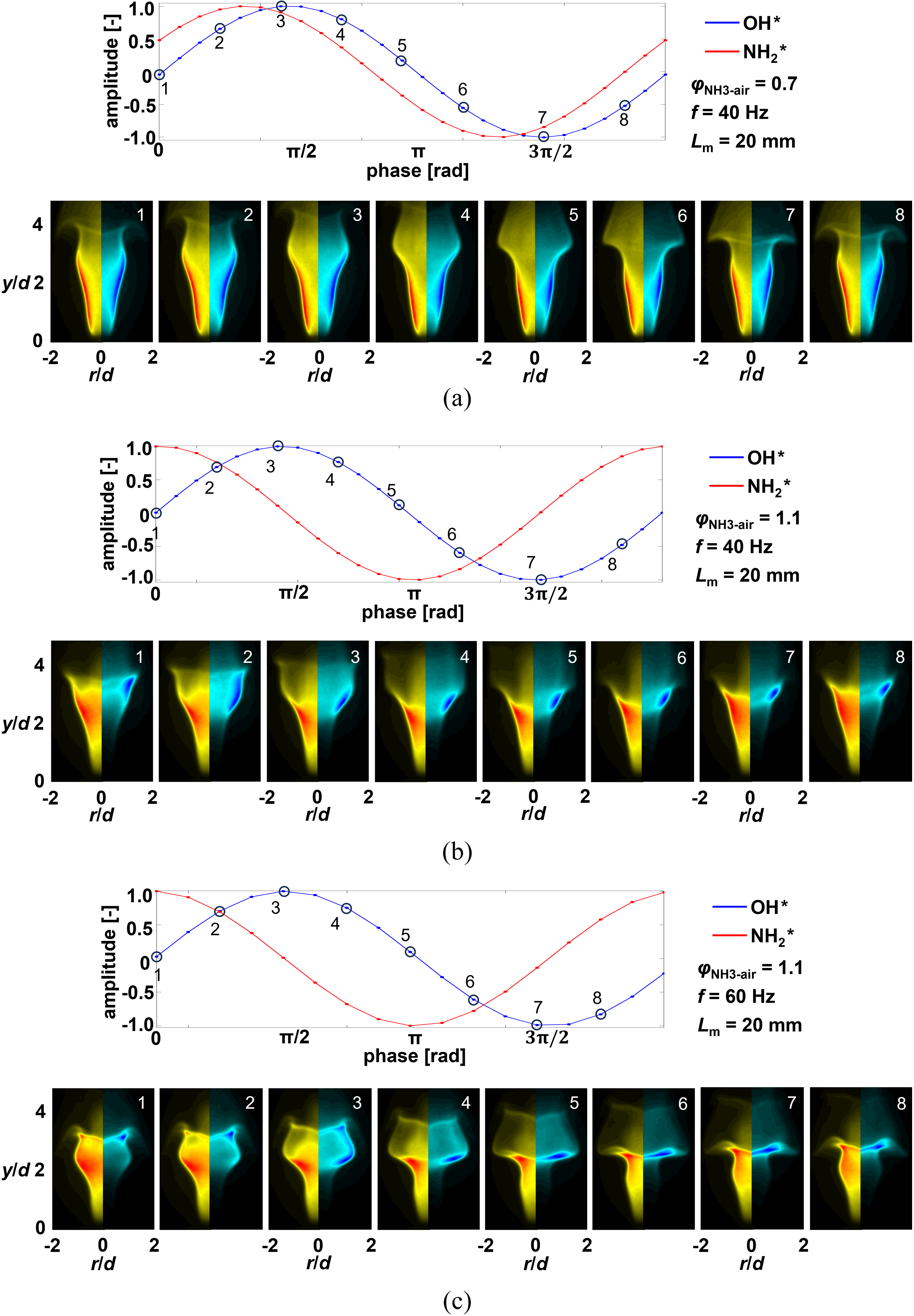
Phase averaged OH*/NH₂* images for (a) ϕ_NH3–air= 0.7, f = 40 Hz, (b) ϕ_NH3–air= 1.1, f = 40 Hz, and (c) ϕ_NH3–air= 1.1, f = 60 Hz corresponding to flames of L_m= 20 mm. (colour online).

Figure 7.

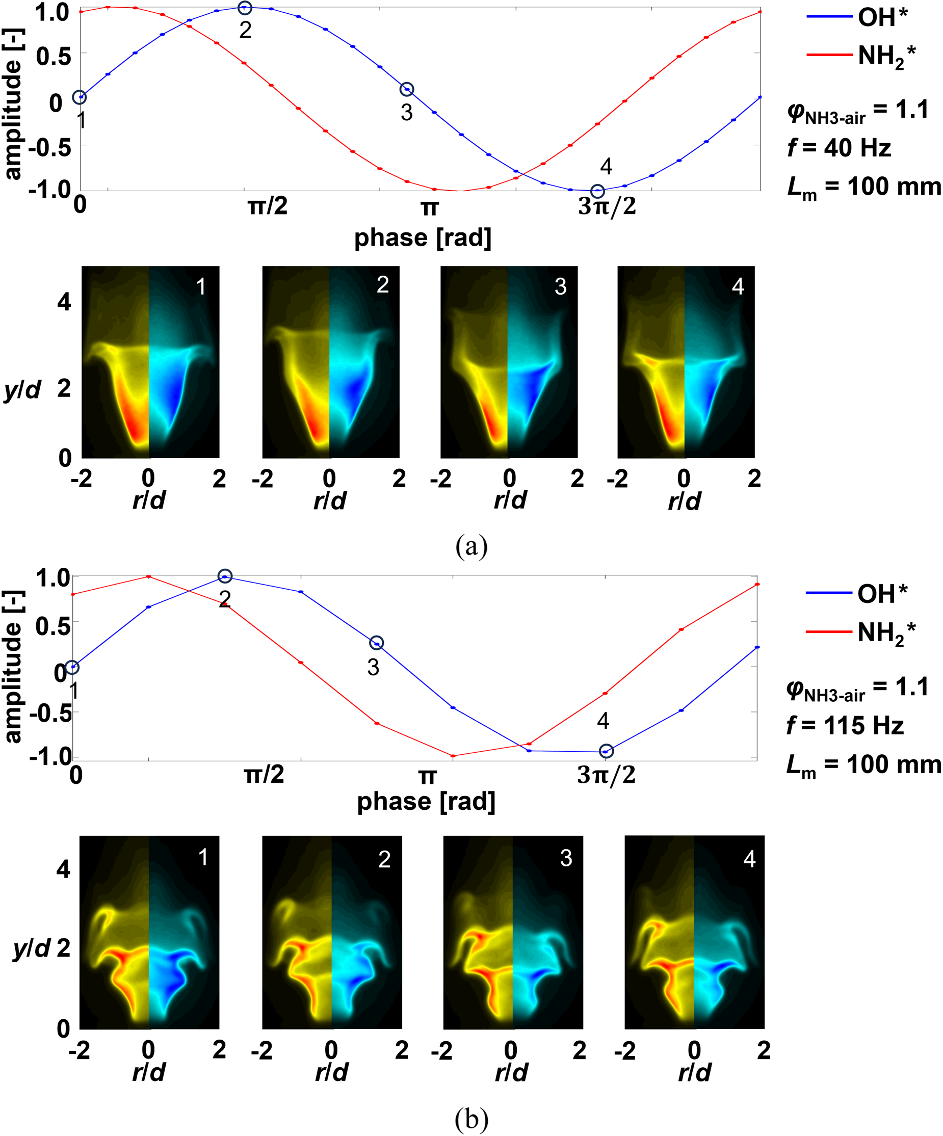
Phase averaged OH* and NH₂* images at forcing frequency of (a) f = 40 Hz, and (b) f = 115 Hz for the flame of ϕ_NH3–air = 1.1 corresponding to L_m= 100 mm. (colour online).

In the phase-averaged images for all the operating conditions and the forcing, flame wrinkling is the main mode of heat release rate oscillations. However, certain features are prevalent depending on the mean I*_OH and I*_NH2 distribution, which are highlighted in the following:

(I) Phase-averaged flames of ϕ_NH3–air= 0.7 and L_m= 20 mm at a frequency of 40 Hz.

Figure 6(a) and (b) shows the phase averaged flames for ϕ_NH3–air= 0.7 and 1.1 for 40 Hz, respectively, for various phases of I*_OH fluctuations. The time series of total NH₂* and OH* fluctuations are obtained by Fourier filtering of the intensity fluctuations at the forcing frequency. The amplitude variation for one cycle of oscillation of I*_OH and I*_NH2 with open circles marked on the I*_OH at the instants at which the phase-averaged flames are shown.

From Figure 6(a) and (b), for ϕ_NH3–air= 0.7 and 1.1, respectively, the flame wrinkle passage results in the overall area fluctuations. Typically, the imposed velocity fluctuations could result in a formation of flow structure in the recirculation region of the dump plane at the vicinity of the flame base³⁷ This results in the perturbation of flame in the form of flame wrinkles. The convection of the incipient flow eventually leads to the propagation of the wrinkles along the flame. The wavelength of the wrinkles on the flame depends directly on the convective speed and inversely on the forcing frequency. In the case of 40 Hz excitation, the estimated wavelength $(λ)$ of the flame wrinkles is ∼ 38 mm (∼3.5d). This is calculated based on the convective velocity scale (U_mean) of 1.5 m/s and the time scale $(τ)$ of 25 ms corresponding to 40 Hz by using the relation $λ = τ$ U_mean. The wrinkle wavelength is comparable to the overall flame length with the flame tip registering significant flapping over various phases compared to the flame base oscillations.

In most phases of the flame oscillations, the flame wrinkling behavior is quite similar for both conditions of ϕ_NH3–air. For ϕ_NH3–air= 0.7 (Figure 6(a)), during the phase of oscillation from 0° towards 90°, the flame shows a bulge around the downstream location of ∼3d from the burner exit with an increase in the total I*_OH and I*_NH2 intensities. As the wrinkle continues further downstream, it is followed by flame necking. The flame necking becomes prominent as the phase approaches 270°. The flame necking is then followed by the flame bulge continuing to the next cycle of oscillation. The alternation of the flame bulge and the flame necking leads to overall flame area oscillations due to the passage of wrinkles resulting in the total intensity fluctuations of the flame radicals. The behavior of the spatial NH₂* follows the behavior of OH* fluctuations except for a phase difference of 30° between the two.

(II) Phase-averaged flames of ϕ_NH3–air= 1.1 and L_m= 20 mm at a frequency of 40 Hz.

Increasing the equivalence ratio to ϕ_NH3–air= 1.1 the changes in the mean flame shape impart a different dynamic behavior. One of the key aspects is that the phase difference between the total OH* and NH₂* is almost 90°, with NH₂* leading the OH*. This could be either due to delayed NH₃ oxidation or cracked NH₃ combustion.

From Figure 6(b), as the flame oscillation commences from the 0° phase, OH* appears as a localized region, while the NH₂* is spread out in its area between 0–4d resulting in its maximum. In this case, the flame is more funnel-shaped with a disparity between the spatial dominance of OH* and NH₂* as discussed before.

As we approach 90° phase with respect to OH*, the funnel-shaped flame increases in its area downstream appearing as a bulge with an elongated OH* region extending to 5d with a less modulated flame base. Following this, the OH* modulation reduces in its amplitude as the flame contraction occurs towards the phase of 270°. The region of higher OH* moves between 3–5d, while for NH₂*, it lies between 2–4d as the phase varies from 90° to 270°. The spatial oscillation of dominant regions of OH* and the NH₂* combined with the flapping of the flame edges resulted in the elongation of I*_OH and I*_NH2 spatial region due to the wrinkles. Both these effects impart the double lobe pattern located at ∼4d which is shown in Figure 5. For the stratified flames, the flame base being narrow, the incipient flow structure could impart lesser influence in these regions. However, the convective growth of the incipient flow structure along the shear layer^36,37 could result in stronger interactions with a wider flame downstream bounded by the wall of the quartz enclosure. This is captured in the amplitude maps which show stronger oscillations in OH* and NH₂* around ∼4d downstream of the burner exit compared to that around the flame base.

Even though the overall flame dynamics of the stratified flames are similar, the changes in the mean flame shape ultimately determine its response to forcing. In this regard, we can see that the flame bulge and necking are common to both the flames in Figure 6(a) and (b). However, for the stratified rich flame, as pointed out before, the peak OH* regions occur ∼4d and are also relatively more localized spatially compared to the lean flame. Since the flame bulge and necking regions coincide with the regions of peak mean OH*, the response of the rich stratified flame is higher compared to the lean stratified flame. This aspect makes the stratified rich flame to be distinct in its flame response even though the basic mechanism is the same.

In addition, for the flames of ϕ_NH3–air= 1.1, one striking feature in the NH₂* field can be observed at the 180° phase (instant 4 in Figure 6(b)). At this condition, the central region in the NH₂* field shows a bulb-like structure downstream, which could be a result of the dominant NH₃–air flame core.

In sum, the peak flame response at 40 Hz for the rich flame is possibly due to the overlap of the peak heat release rate location with the region of significant flame flapping. As pointed out earlier, the flame response is a function of the flame shape and the wrinkle length scale that depends on the frequency.

(III) Phase-averaged flames of ϕ_NH3–air= 1.1 and L_m= 20 mm at a frequency of 60 Hz.

As we increase the forcing frequency to 60 Hz while, retaining ϕ_NH3–air= 1.1, the wavelength of the wrinkle reduces to 25 mm (∼2d). However, the phase difference between the OH* and NH₂* remains ∼ 90° like before as shown in Figure 6(c). This implies that the phase difference between the radical intensity fluctuations is driven by the stratification effects for the frequencies that show relatively higher flame response.

The phase-averaged images are presented in Figure 6(c). Most of the overall flame dynamics between cases with different frequencies remain unaltered. Unlike the forcing at 40 Hz, the flame base is relatively more active during the growth phase of the oscillation from 0° to 90°, which is associated with the reduced length scale of the flow structure. Further, the OH* regions elongate, and it is spread around the central regions of the flame compared to the previous case. The NH₂* is contained within 4d from the burner exit and has begun to reduce in its intensity.

Towards the OH* minimum (270° phase), the flame approaches a flower vase shape with the spatial NH₂* intensities tending towards its maximum. As far as the NH₂* minimum (180° phase of OH*), the central region of the NH₃–air flame reflects a bulb shape similar to that observed in the previous case.

(IV) Phase-averaged flames of ϕ_NH3–air= 1.1 and L_m= 100 mm at the frequency of 40 Hz.

For the unstratified flame, we discuss the effect of forcing frequencies of 40 and 115 Hz on the flame behavior. The flame wrinkle modulation behavior for the unstratified flame is similar to that for the stratified flames. Owing to this, we show phase-averaged images only for four phases from 0° to 90° spaced apart by 90° in the interest of brevity. The phase-averaged images for the forcing frequency are shown in Figure 7(a) for the unstratified flame corresponding to ϕ_NH3–air= 1.1. An increase in the premixedness of the incoming reactants due to a higher mixing length increases the flame cone angle and decreases the overall flame length. The length scale of the wrinkles for 40 Hz forcing is 38 mm (∼3.5d) as before.

At the phase of 0°, the flame is more tulip-shaped compared to the funnel-shaped stratified flames of the same power. Both the OH* and NH₂* are prevalent around the bluff body vicinity and extend to a downstream location of ∼3.5d. The flame tip is relatively curved at its edges, which could be influenced by the recirculation zone. Towards the phase of 90°, the overall flame length increases as the curved flame tip moves downstream. This is accompanied by an increase in the spatial spread of radicals as the flame bulges out. The spatial locations of dominant OH* and NH₂* do not vary compared to those at 0°. This contrasts with the stratified flame, where the peak spatial location of the flame radicals varies over one cycle of flame oscillation.

From 90° to 270° the tulip-shaped flame switches to a conical shape. At the phase of 270°, the flame height is minimum with the flame tip having a smaller standoff from the quartz liner along with a smaller spatial spread of the I*_OH and I*_NH2. Furthermore, the phase difference between I*_OH and I*_NH2 is around 50° compared to the stratified flames as seen before.

Even though the flame wrinkle wavelength is the same as before for 40 Hz forcing frequency, the modulation of peak OH* and NH₂* of the flame is weaker in the unstratified flame compared to the stratified flame of the same power. This difference arises from the relatively uniform spatial intensity of flame radicals compared to a more localized distribution located in the regions of flame wall interaction of intensity of the stratified. This in turn results in a stronger OH* response of the stratified flame compared to that of the unstratified flame reflecting the impact of mixture tailoring.

(V) Phase-averaged flames of ϕ_NH3–air= 1.1 and L_m= 100 mm at the frequency of 115 Hz.

For the forcing frequency of 115 Hz, the length scale of the perturbation is estimated to be approximately 15 mm (∼1.3d), which is shorter than the flame length resulting in a significant wrinkling of the flame. The flame response is comparable to the response at a lower frequency compared to the stratified flames. Additionally, the phase difference between the OH* and NH₂* is lower than the rich stratified flame and is estimated to be ∼50° shown in Figure 7(a).

In the phase-averaged images shown in Figure 7(b), moving from 0° towards 90° phase in the OH* fluctuation, both the OH* and NH₂* regions occupy the flame region covering 0–4d from the bluff body. The flame base exhibits significant variation in its area. For instance, at 90° the flame develops a bulge compared to that observed at 0° at its base, which tends to convectively amplify resulting in the flame wrinkling as the phase increases. The passage of the small-scale wrinkles and flame height fluctuations results in the variation of total OH*/NH₂*.

Typically, the oscillations of the flame cone angle at its base and passage of wrinkle along the downstream locations of the flame result in the double lobe pattern reflected by the amplitude map shown in Figure 5 for the forcing frequencies of 40 and 100 Hz. The length scale of the double lobe observed in the amplitude map is determined by the wrinkle length. The oscillations of the distributed I*_OH and I*_NH2 over the entire flame length result in an elongated double lobe structure for the unstratified flames. This behavior contrasts that observed in the stratified flames of the same power but with localized OH* and NH₂*regions.

In summary, the flame response for the L_m= 100 mm case at the forcing frequency of 115 Hz is attributed to both flame wrinkling and flame base oscillations compared to the forcing frequency of 40 Hz that accompanies a large-scale flame flapping. However, for the flame of L_m= 20 mm, the oscillations in the localized flame radical emissions along with the overall flame area fluctuation due to the flame flapping could play a role in the flame dynamics and response. Apart from the flame area oscillations, the stratification effects can also contribute to the flame response, especially for the flames of L_m= 20 mm.

Effect of stratification on the nature of I*_OH fluctuations

A comparison of total I*_OH fluctuations is shown in Figure 8 to point out the impact of stratification. For each case, we use the unfiltered chemiluminescence intensity fluctuation signals unlike that shown in Figures 6 and 7. We consider the stratified flames corresponding to L_m= 20 mm at 40 Hz for ϕ_NH3–air= 0.7 and 1.1 and that for L_m= 100 mm at frequencies of 40 and 115 Hz.

Figure 8.

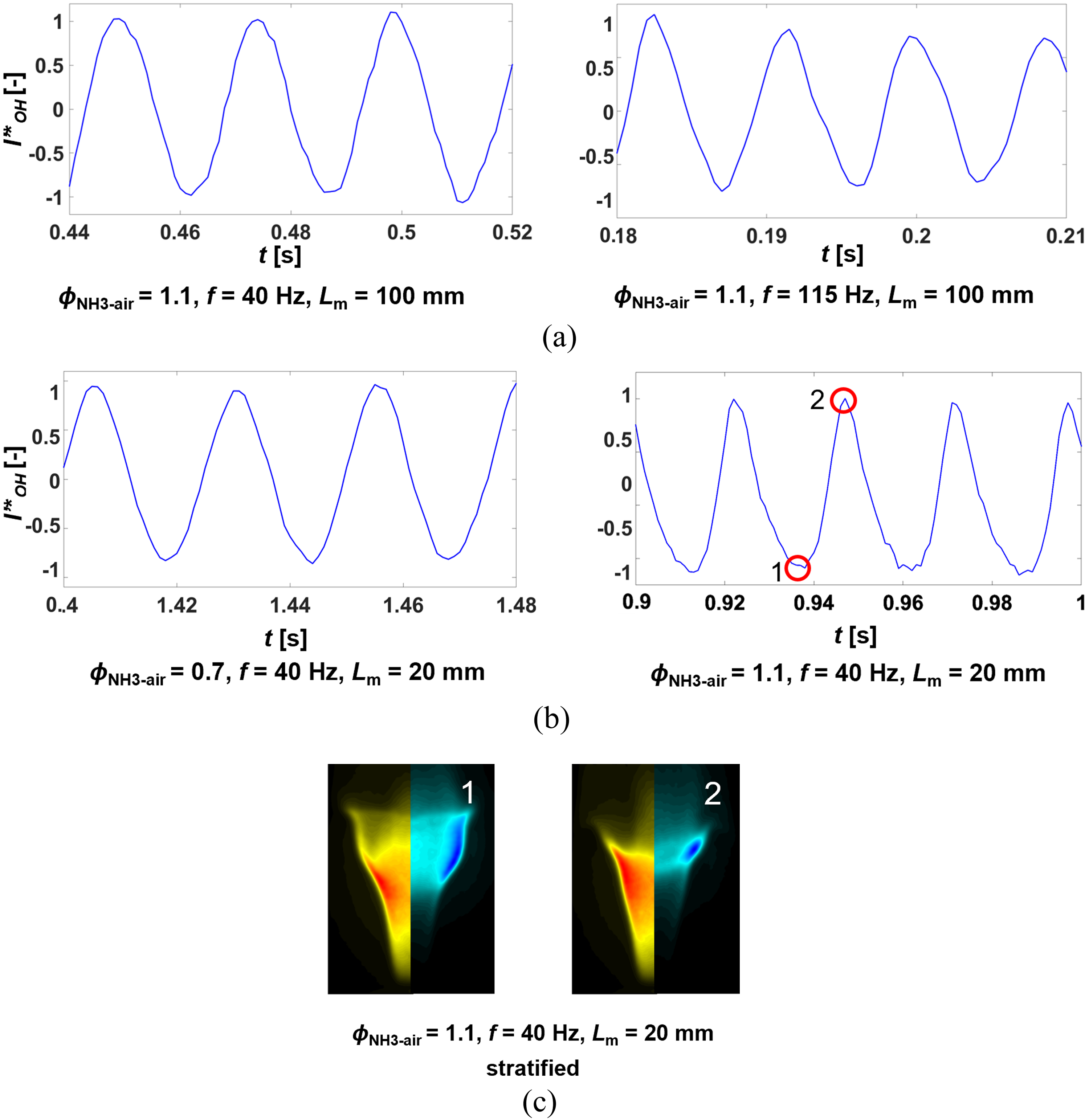
Total normalized OH* fluctuations for (a) L_m= 100 mm, (b) L_m= 20 mm, and (c) instantaneous I*_OH and I*_NH2 images for the flame of L_m= 20 mm at time instants marked as 1 and 2 in (b). (colour online).

For the unstratified flame of L_m= 100 mm forced at 40 and 115 Hz, the fluctuations I*_OH are comparable and quite sinusoidal as depicted in Figure 8(a). However, for the stratified flame for L_m= 20 mm in Figure 8(b), the I*_OH fluctuations are sinusoidal at 40 Hz for the lean condition similar to that for the rich unstratified flames. For the same stratification, as we increase ϕ_NH3–air to 1.1, the signature of I*_OH fluctuations is observed to deviate from the sinusoidal ones. The oscillatory pattern exhibits a faster crest and slower trough, which resembles reversed saw-tooth oscillations.

Such a non-sinusoidal pattern for the rich stratified flame is due to the coincidence of regions of peak flame flapping with the regions of peak flame OH* emission. This fact is emphasized in the flame OH* distribution shown in Figure 8(c), which shows significant modulation of peak OH* regions. But in the unstratified rich flame and stratified lean flame, even though the flame flapping is prevalent, the spatial flame radical distribution is uniform resulting in a more sinuous pattern affirming the role of mean flame shapes in the flame response.

The velocity perturbation at the exit of the burner results in a flow structure roll-up at the flame base, which convects and amplifies in the dump plane resulting in wrinkles on the flame surface. Since the flame base is narrow and the reactant mixture is rich, the flow roll-up would entrain the unburnt reactant that it transports downstream. It is shown in Figure 4 that in the rich stratified flame the OH* is more localized compared to the lean stratified flames or the unstratified flames of the same power at the downstream location of ∼4d from the burner exit. As the unburnt reactant within the flow roll-up encounters the concentrated OH* region, the combustion of the entrained reactant could occur in a rapid manner similar to vortex combustion.³⁷ This in turn results in a faster increase in the OH* giving rise to the reverse saw-tooth type oscillation.

I_OH–I_NH2 phase difference variation (Δθ_OH–NH2)

In the last part of this study, we present the phase difference variation for flames with different stratification and equivalence ratios in Figure 9. For this, we consider two forcing frequencies namely, 40 and 60 Hz for which all the flames show comparable responses.

Figure 9.

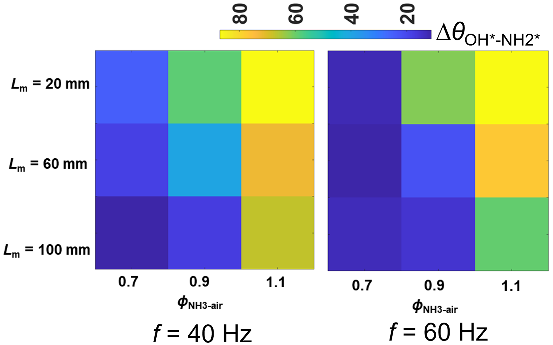
The phase difference between I*_OH and I*_NH2 for two forcing frequencies and different operating conditions of the flame indicated on the axes.

We have seen that for both the forcing frequencies, increasing ϕ_NH3–air results in an increase in the phase difference between the oscillations in OH* and NH₂* for any mixing length. This is related to the increase in the disparity in the spatial dominance of OH* and NH₂*. Likewise increase in the stratification (decrease in L_m) at a particular ϕ_NH3–air results in increased phase difference between the two radicals.

As pointed out earlier, increased stratification results in poor mixing of NH₃–air with H₂–air and hence increased time scales of the reaction resulting in a larger phase delay. Another aspect is that the increase in the phase delay is highest for the stratified flame compared to the unstratified ones implying the dominance of stratification over the ϕ_NH3–air effect. Thus, combining both effects, we see that flames of richer ϕ_NH3–air and highest stratification generate the largest phase difference between the OH* and NH₂* fluctuations.

Conclusions

In this study, we investigate bluff body-stabilized laminar ammonia hydrogen flames with stratification to highlight its impact on flame oscillations and spatial flame dynamics. The reactant streams, NH₃–air and H₂–air are issued into two annular passages formed by (a) the inner and outer tubes and (b) the inner tube and the bluff body. The stratification is controlled by retracting the inner tube relative to the burner exit, which controls the mixing between the NH₃–air and H₂–air. The HWA measurements, and high-speed imaging of radicals such as I*_OH and I*_NH2 are performed. For the unforced non-reacting flow, the measured velocity fluctuations at the burner exit correspond to intensities of ∼ 0.5% with broadband spectra that are insignificant compared to the forcing amplitudes.

The key aspects of tailoring NH₃–H₂ blends on the flame behavior are as follows:

For the unforced flames of ϕ_NH3–air= 1.1 and L_m= 20 mm, the mean I*_OH and I*_NH2 are spatially compact compared to the leaner and less stratified flames for the same flame power.

The amplitude map of the forced flame reflects the strength of I*_OH and I*_NH2 fluctuations to be higher along the flame boundary for the lean, unstratified conditions. This tends to become dominant towards the central regions of the flame in the downstream locations resulting in double lobe patterns located at∼2–4d with increasing stratification and ϕ_NH3–air.

Forcing at a lower frequency for the rich stratified flame results in dominant flame tip oscillations that coincide with oscillations of the peak spatial NH₂* and OH* locations, unlike the rich unstratified flame. The unstratified flame forced at a higher frequency accompanies flame base oscillations and wrinkle propagation to contribute to the overall heat release rate variations. The relationship between the spatial flame fluctuations and heat release rate distribution governs the flame response frequencies.

The flame tip oscillation coinciding with the peak OH* region registers non-sinusoidal oscillations of the rich stratified flame compared to the lean stratified flame and rich unstratified flame that reflects sinuous oscillations.

Further, the phase difference between the OH* and NH₂* oscillations is ∼ 90° for the rich and stratified flames, while it reduces with leaner flames with reduced stratification.

In sum, the flame dynamics of NH₃–H₂ blends are modified due to the stratification effects through changes in the spatial distribution of flame radicals, which govern the flame shape. An increased stratification leads to a shift in flame response toward lower frequencies compared to flames with lower stratification. This study needs to be extended to estimate the flame transfer function with a smaller frequency resolution of forcing to extract the true nature of stratification.

Footnotes

Acknowledgments

The present research is supported by the Competitive Research Grant funding from King Abdullah University of Science and Technology (KAUST) under grant number URF/1/4051-01-01.

Declaration of conflicting interests

The author(s) declared no potential conflicts of interest with respect to the research, authorship, and/or publication of this article.

Funding

The author(s) disclosed receipt of the following financial support for the research, authorship, and/or publication of this article: This work was supported by the King Abdullah University of Science and Technology (grant number URF/1/4051-01-01).

ORCID iD

Ramgopal Sampath

References

Valera-Medina

Xiao

Owen-Jones

, et al. Ammonia for power. Prog Energy Combust Sci 2018; 69: 63–102.

Kobayashi

Hayakawa

Kunkuma

, et al. Science and technology of ammonia combustion. Proc Combust Inst 2019; 37: 109–133.

Huang

Kobayashi

, et al. Numerical study on effect of oxygen content in combustion air on ammonia combustion. Energy 2015; 93: 2053–2068.

Shrestha

Lhuillier

Barbosa

, et al. An experimental and modeling study of ammonia with enriched oxygen content and ammonia/hydrogen laminar flame speed at elevated pressure and temperature. Proc Combust Inst 2021; 38: 2163–2174.

Chen

Zhang

, et al. Effect and mechanism of combustion enhancement and emission reduction for non-premixed pure ammonia combustion based on fuel preheating. Fuel 2022; 308: 122017.

Chen

Sui

, et al. Flame and emission characteristics of preheated ammonia combustion based on chemical reaction network. Fuel Process Technol 2023; 242: 107652.

Pugh

Valera-Medina

Bowen

, et al. Emissions performance of staged premixed and diffusion combustor concepts for an NH₃/air flame with and without reactant humidification. J Eng Gas Turbines Power 2021; 143: 051012.

Lee

Guahk

Kim

, et al. Stability and emission characteristics of ammonia-air flames in a lean-lean fuel staging tangential injection combustor. Combust Flame 2023; 248: 112593.

Heggset

Meyer

OHH

Tay-Wo-Chong

, et al. Numerical assessment of a Rich-Quench-Lean staging strategy for clean and efficient combustion of partially decomposed ammonia in the constant pressure sequential combustion system. J Eng Gas Turbines Power 2024; 146: 081004.

10.

Okafor

Somarathne

KDKA

Hayakawa

, et al. Towards the development of an efficient low-NOx ammonia combustor for a micro gas turbine. Proc Combust Inst 2019; 37: 4597–4606.

11.

Chen

Liu

Zhao

, et al. Experimental and chemical kinetic study on the flame propagation characteristics of ammonia/hydrogen/air mixtures. Fuel 2023; 334: 126509.

12.

Wang

Huang

Zhang

, et al. Laminar burning characteristics of ammonia/hydrogen/air mixtures with laser ignition. Int J Hydrogen Energy 2021; 46: 31879–31893.

13.

Mashruk

Zitouni

Brequigny

, et al. Combustion performances of premixed ammonia/hydrogen/air laminar and swirling flames for a wide range of equivalence ratios. Int J Hydrogen Energy 2022; 47: 41170–41182.

14.

Valera-Medina

Gutsea

Xiao

, et al. Premixed ammonia/hydrogen swirl combustion under rich fuel conditions for gas turbines operation. Int J Hydrogen Energy 2019; 44: 8615–8626.

15.

Ånestad

Sampath

Moeck

, et al. The structure and stability of premixed CH4, H2, and NH3/H2 flames in an axially staged can combustor. In: Proceedings of ASME turbo expo, turbomachinery technical conference and exposition, 2023, GT2023-103088.

16.

Mashruk

Kovaleva

Alnasif

, et al. Nitrogen oxide emissions analyses in ammonia/hydrogen/air premixed swirling flames. Energy 2022; 260: 125183.

17.

Zhu

Khateeb

Guiberti

, et al. NO and OH* emission characteristics of very-lean to stoichiometric ammonia–hydrogen–air swirl flames. Proc Combust Inst 2021; 38: 5155–5162.

18.

Mashruk

Alnasif

, et al. Combustion characteristics of a novel ammonia combustor equipped with stratified injection for low emission. J Ammonia Energy 2023; 01: 21–32.

19.

Jin

Kim

. Hybrid rich- and lean-premixed ammonia-hydrogen combustion for mitigation of NOx emissions and thermoacoustic instabilities. Combust Flame 2024; 262: 113366.

20.

Vermeulen

Danilowich

HeydEauff

, et al. The acoustically excited flame. J Eng Power 1976; 98: 147–157.

21.

Yoon

. Thermoacoustics and combustion instability analysis for multi-burner combustors. J Sound Vib 2021; 492: 115774.

22.

Kim

Lee

Quay

, et al. Spatially distributed flame transfer functions for predicting combustion dynamics in lean premixed gas turbine combustors. Combust Flame 2010; 157: 1718–1730.

23.

Schuller

Durox

Candel

. A unified model for the prediction of laminar flame transfer functions: comparisons between conical and V-flame dynamics. Combust Flame 2003; 134: 21–34.

24.

Candel

. Combustion dynamics and control: progress and challenges. Proc Combust Inst 2002; 29: 1–28.

25.

Kim

Lee

, et al. Characterization of forced flame response of swirl-stabilized turbulent lean-premixed flames in a gas turbine combustor. J Eng Gas Turbines Power 2010; 132: 041502.

26.

Kim

Park

. Effects of hydrogen addition on flame structure and forced flame response to velocity modulation in a turbulent lean premixed combustor. Fuel 2010; 89: 3475–3481.

27.

Sabatino

Guiberti

Moeck

, et al. Fuel and equivalence ratio effects on transfer functions of premixed swirl flames. J Propul Power 2020; 36: 271–284.

28.

Gatti

Gaudron

Mirat

, et al. Impact of swirl and bluff-body on the transfer function of premixed flames. Proc Combust Inst 2019; 37: 5197–5204.

29.

Wiseman

Gruber

Dawson

. Flame transfer functions for turbulent, premixed, ammonia-hydrogen-nitrogen-air flames. J Eng Gas Turbines Power 2023; 145: 031015.

30.

Nunes

Morgans

. The acoustic response of hydrogen/ammonia flames. J Ammon Energy 2023; 01: 033–045.

31.

Katoch

Guiberti

De Campos

, et al. Dual-fuel, dual-swirl burner for the mitigation of thermoacoustic instabilities in turbulent ammonia-hydrogen flames. Combust Flame 2022; 246: 112392.

32.

Chi

Sreekumar

Thévenin

. Data-driven discovery of heat release rate markers for premixed NH₃/H₂/air flames using physics-informed machine learning. Fuel 2022; 330: 125508.

33.

Otomo

Koshi

Mitsumori

, et al. Chemical kinetic modeling of ammonia oxidation with improved reaction mechanism for ammonia/air and ammonia/hydrogen/air combustion. Int J Hydrogen Energy 2018; 43: 3004–3014.

34.

Shanbhogue

Shin

D-H

Hemchandra

, et al. Flame sheet dynamics of bluff-body stabilized flames during longitudinal acoustic forcing. Proc Combust Inst 2009; 32: 1787–1794.

35.

Gabruk

Roe

. Velocity characteristics of reacting and nonreacting flows in a dump combustor. J Propul Power 1994; 10: 148–154.

36.

Sampath

Chakravarthy

. Investigation of intermittent oscillations in a premixed dump combustor using time-resolved particle image velocimetry. Combust Flame 2016; 172: 309–325.

37.

Ayache

Dawson

Triantafyllidis

, et al. Experiments and Large-Eddy simulations of acoustically forced bluff-body flows. Int J Heat Fluid Flow 2010; 31: 754–766.

Effect of stratification on the combustion behavior and dynamic response of a bluff-body stabilized ammonia–hydrogen flames with radial staging

Abstract

Keywords

Introduction

Experimental setup and operating conditions

Measurement techniques

Calibration procedure for the forcing tests

Results and discussion

Unforced flow spectrum

The flame response of forced flames

Flame visualization

Time-averaged unforced flames

Amplitude map of forced flames

Phase averaged NH2* and OH* fields

Effect of stratification on the nature of I*OH fluctuations

I*OH–I*NH2 phase difference variation (ΔθOH*–NH2*)

Conclusions

Footnotes

Acknowledgments

Declaration of conflicting interests

Funding

ORCID iD

References

Phase averaged NH₂* and OH* fields

Effect of stratification on the nature of I*_OH fluctuations

I_OH–I_NH2 phase difference variation (Δθ_OH–NH2)