Sage Journals: Discover world-class research

Abstract

Modelling the flame response of turbulent flames via data-driven approaches is challenging due, among others, to the presence of combustion noise. Neural network methods have shown good potential to infer laminar flames’ linear and nonlinear flame response when externally forced with broadband signals. The present work extends those studies and analyses the ability of neural network models to evaluate the linear and nonlinear flame response of turbulent flames. In the first part of this work, the neural network is trained to evaluate and interpolate the linear flame response model when presented with data obtained at various thermal conditions. In the second part, the neural network is trained to infer the nonlinear flame response model when presented with time series exhibiting sufficient large amplitudes. In both cases, the data is obtained from a large eddy simulation of an academic combustor when acoustically forced by broadband signals.

Keywords

Turbulent flame response flame transfer function flame describing function neural network models

Introduction

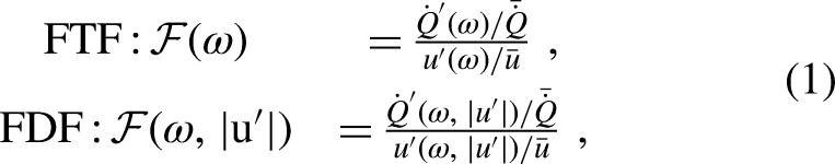
Over the last decades, stringent emission regulations have led to the development of new clean combustion technologies, such as lean premixed combustion. This development enhances the risk of thermoacoustic instabilities, which can damage the engines severely.¹ Therefore, it is desirable to predict these instabilities during the design phase. For such a goal, a reliable model of the flame response to acoustic oscillations^2–4 is generally necessary. A well-established strategy to model such linear and non-linear flame responses is using the flame transfer function (FTF) and flame describing function (FDF), respectively. These transfer functions relate the fluctuations of heat release rate, ${\dot{Q}}^{'}$ , produced as a response to upstream velocity perturbations, $u^{'}$ , by

\begin{matrix} FTF : F (ω) & = \frac{{\dot{Q}}^{'} (ω) / \bar{\dot{Q}}}{u^{'} (ω) / \bar{u}}, \\ FDF : F (ω, | u^{'} |) & = \frac{{\dot{Q}}^{'} (ω, | u^{'} |) / \bar{\dot{Q}}}{u^{'} (ω, | u^{'} |) / \bar{u}}, \end{matrix}

(1)

where

\bar{(\cdot)}

and

(\cdot)^{'}

denote temporal averaging and fluctuations, respectively. The FTF is a linear description of input to ouput mapping, which is valid only in the limit of small acoustic perturbations. Suppose large amplitudes of acoustic perturbations are considered. In that case, the flame response becomes nonlinear, requiring a nonlinear flame description such as the FDF,⁵ as shown in equation (1). Note that the FDF model is restrictive as it assumes that the flame responds exclusively at the same frequency as the input signal

u^{'}

. Haeringer et al.⁶ and Orchini et al.⁷ proposed an extended FDF and the flame double input describing function approaches, respectively, to permit responses that exhibit frequencies that are additional (combination of fundamental and harmonics) to the fundamental one.

Large eddy simulation (LES) is a widely used approach for numerical analysis of turbulent combustion systems. Many simulations may be performed over a desired range of frequencies and amplitudes in the input to obtain a corresponding flame response.⁸ A conventional approach of obtaining FDF relies on harmonic excitation of the inlet velocity. Such an approach requires multiple computational fluid dynamics (CFD) simulations to calculate the flame response, which is computationally expensive. As a result, developing a methodology to compute the flame response using a single CFD simulation is advantageous.

Polifke et al.⁹ proposed combining CFD and system identification (SI) to characterize the linear flame response to incoming flow perturbations. The CFD simulation is performed by exciting a flame with a low-pass filtered, broadband signal of upstream acoustic velocity perturbations. The resulting time series of fluctuating heat release rate ${\dot{Q}}^{'}$ and inlet velocity $u^{'}$ are used to identify the linear flame response, i.e., the impulse response and corresponding frequency response (FTF) using correlation analysis. Even though this approach models an FTF from a single simulation, it is limited to the linear flame response. Modelling the nonlinear flame response^2,5 remains unattainable for such correlation approaches.

Neural network (NN) models can be used to capture the nonlinear relationships in the data¹⁰ and are found to be useful in the field of fluid dynamics.^11–13 Among the first works related to thermoacoustics, Förner and Polifke¹⁴ modelled the nonlinear acoustic behaviour of Helmholtz resonators using a data-based, reduced-order model. The data coming from CFD simulation was used to train a local-linear neurofuzzy network. Jaensch and Polifke¹⁵ proposed a NN-based approach for reacting flows, where they attempted to model the FDF of a slit laminar flame.¹⁶ The results of that study were not satisfactory, perhaps because of the lack of regularization techniques, such as dropout or L-norms, or because of the use of shuffling in the data.¹⁷ In subsequent work, Tathawadekar et al.¹⁸ demonstrated the use of multi-layer perceptron (MLP), the same type of NN model used in Förner and Polifke,¹⁵ to characterize the nonlinear flame response of a laminar flame. When combined with an acoustic solver, the trained NN model was able to predict limit-cycle amplitudes accurately. Yadav et al.¹⁹ applied the long short-term memory (LSTM) model, a type of recurrent NN, to predict the nonlinear flame response of a laminar flame. They show that LSTM may be advantageous, as they require shorter time series if compared with the MPL counterparts. However, to this day, LSTM models have not yet been validated for predicting flame responses at amplitudes higher than 0.5, nor for estimating limit cycle oscillations when coupled with a given acoustic solver.

Following Tathawadekar et al.,¹⁸ the present work extends the applicability of NNs to model the linear and nonlinear flame response of turbulent flames. We demonstrate the flexibility of the NN model in two cases of interest. In the first case, we consider predicting the linear flame response under varying thermal conditions at a given boundary. As such, the temperature at the combustion chamber’s back plate is considered a variable. The NN model is trained on a few data-sets of broadband excited simulations with varying back plate temperatures. The trained NN model is then used to predict the flame response of the burner configuration characterized by an unseen back-plate temperature. The second case focuses on training and testing a NN model to characterize the linear and nonlinear flame response belonging to a turbulent swirled combustor.

Numerical setup

The present work investigates the flame dynamics of two turbulent, swirl-stabilized combustors: the fully premixed EM2C and ETH burners. Schematic representations of both are given in Figures 1 and 2, where the computational domains are highlighted in colour. Geometrical and numerical details of both burners are summarized in Table 1. The numerical validation of the EM2C burner was carried out by Merk et al.²³ and Kulkarni et al.²⁴ – for more information, the reader is referred to these works. The combustor back plate was defined as a no-slip isothermal wall. In the work of Kulkarni et al.,²⁴ the back plate temperature of the combustor is varied in the range of 700–960 K to quantify the uncertainty in the flame response model. The respective data is used for further analysis to predict the FTF with the present NN model at unseen boundary conditions.

The LES of the ETH burner²⁵ is performed using the finite volume-based OpenFOAM 10 library²⁶ solving the reactive Navier-Stokes equations. To decouple acoustics and flame response and therefore avoid self-excited instabilities or resonances in the system,²⁷ a low Mach number formulation of the reactingFoam solver is utilized in the present work. The time integration is achieved using a fully-implicit, second-order accurate Euler scheme. The PISO-consistent algorithm solves the velocity-pressure coupling with three inner iterations. The time step is $Δ t = 10^{- 6}$ s, which assures a Courant-Friedrichs-Lewy (CFL) number below 0.3 in the flame region. The numerical domain is discretized with 6 million hexahedral elements and is refined in the swirler and flame region. The boundary conditions consist of velocity inlet and total pressure outlet, while all walls are treated as no-slip. Isothermal walls with a fixed temperature of 700 K are set for the combustor walls and bluff body plane. The WALE²⁰ sub-grid scale model accounts for small-scale fluid motions. An extended version of the dynamic thickened flame model²¹ is utilized to consider turbulence-flame interaction. The two-step global mechanism BFER by Franzelli et al.²² is applied for modelling chemical reactions. The species and energy equations are modelled with a unity Lewis number and a mixture Prandtl number of $Pr = 0.7$ , a common approximation in hydrocarbon combustion.

Figure 1.

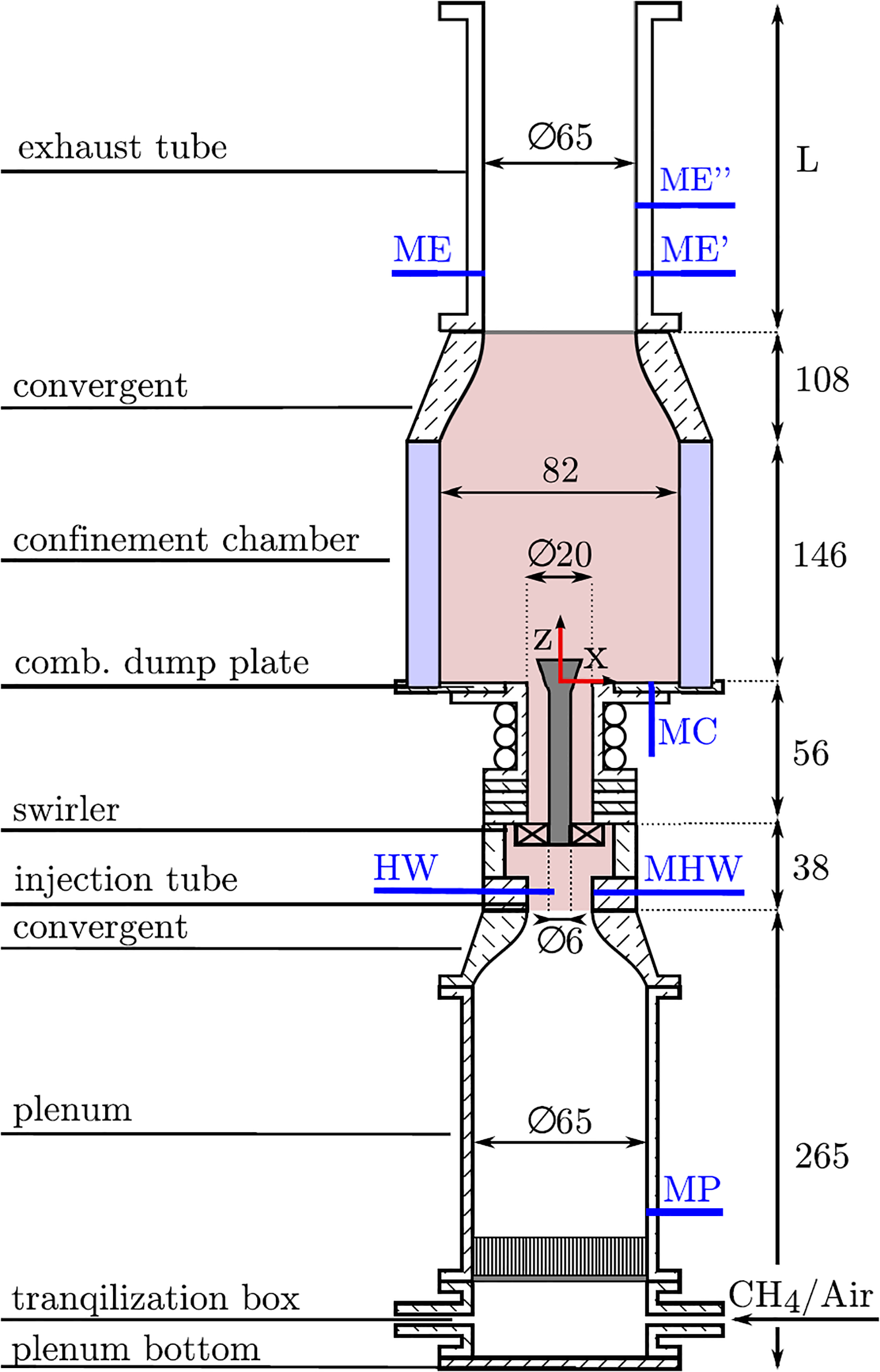
Schematic of the EM2C turbulent swirl combustor. Dimensions are given in millimeters. Figure adapted from Merk et al.²³

Figure 2.

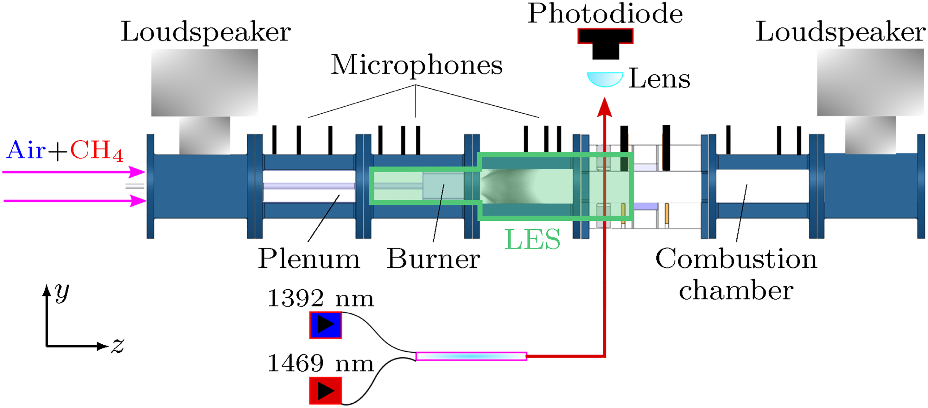
Schematic of the ETH turbulent swirl combustor. Figure adapted from Eder et al.²⁵

Table 1.

The two burners under investigation.

Name	EM2C	ETH
LES code	AVBP	OpenFOAM
	(fully comp.)	(low Mach)
Subgrid model	WALE	WALE
(Nicoud and Ducros 1999²⁰)
Combustion model	DTFLES	DTFLES
(Colin et al. 2002²¹)
Chemistry scheme	2S-BFER	2S-BFER
(Franzelli et al. 2012²²)
Mesh size	19 $\times$ 10⁶	6 $\times$ 10⁶
Swirler	radial	axial
Fuel	CH₄	CH₄
$P_{th}$ [kW]	5.5	48
$ϕ$ [-]	0.82	0.77

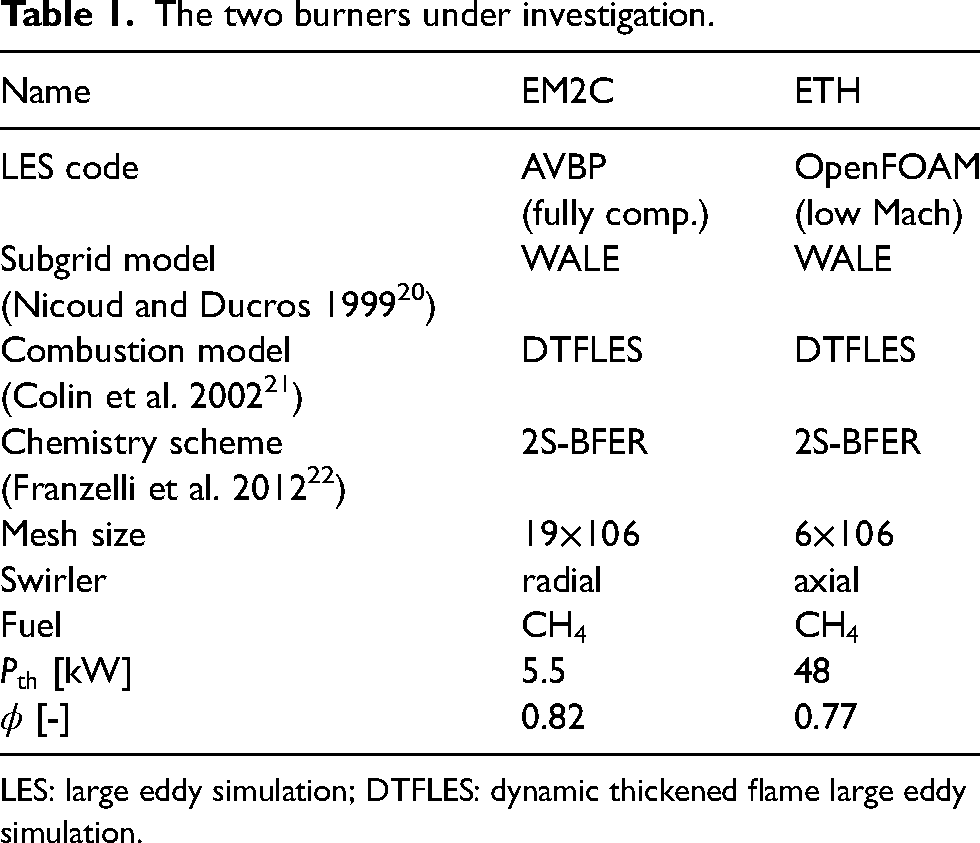
LES: large eddy simulation; DTFLES: dynamic thickened flame large eddy simulation.

Methodology

In this section, we formalize the problem statement, provide the pre-processing of data and details of the NN model.

EM2C burner: Problem formulation

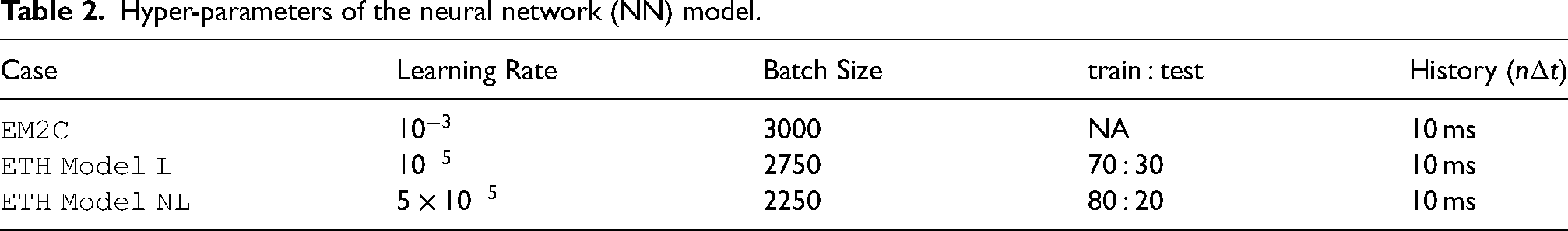
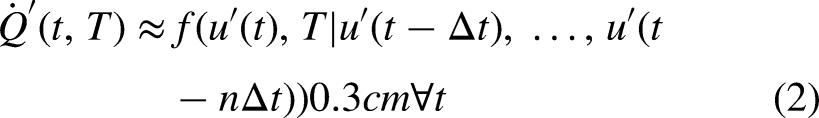
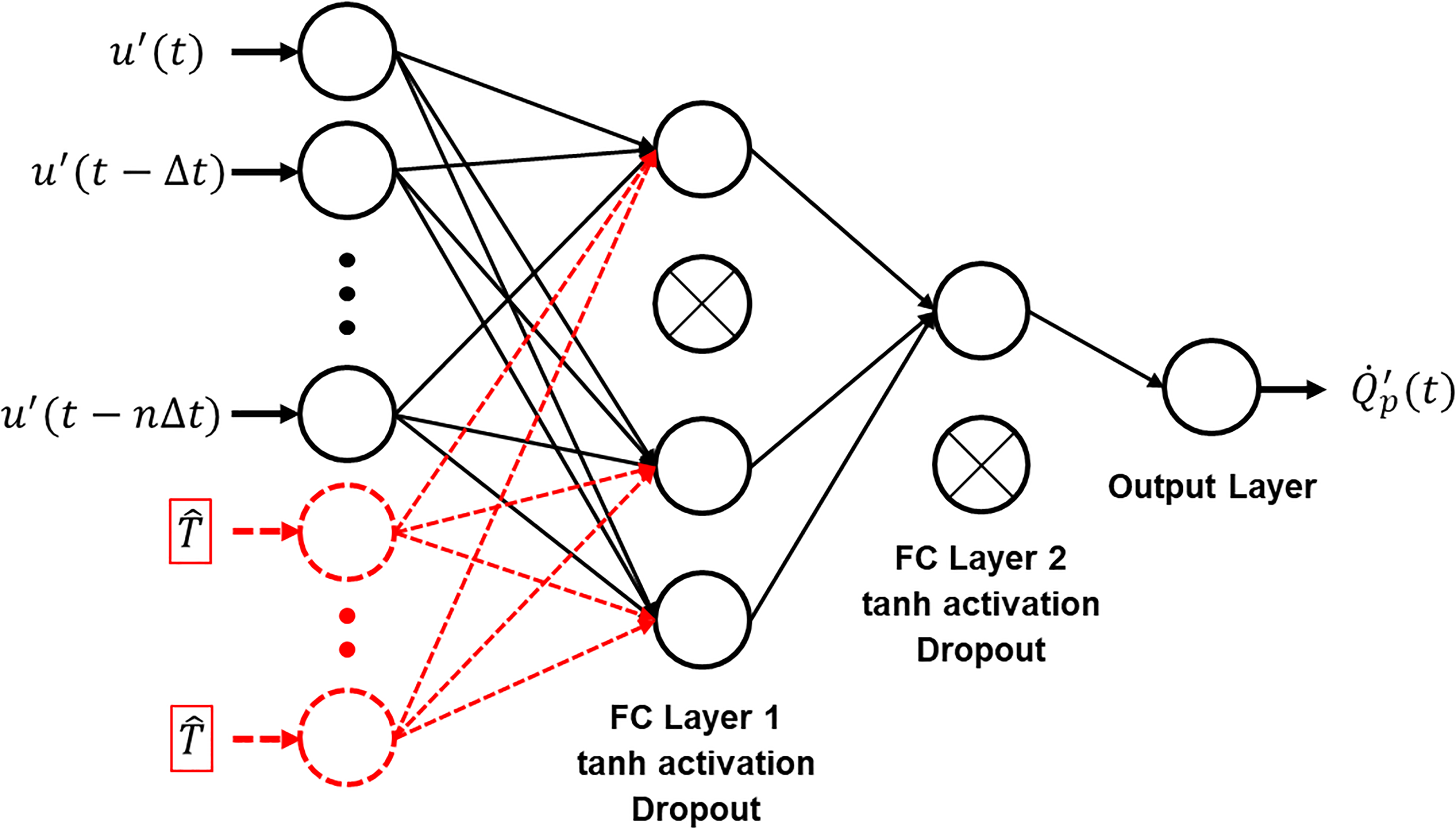
Using the EM2C burner, LES simulations are carried out for 12 different back-plate temperatures in the range of 700–960K. Each simulation generates the time series of broadband, low-pass filtered velocity signal and corresponding heat release rate fluctuations. The NN model is trained to predict the heat release rate fluctuations given the data of inlet velocity and the back plate temperature ( $T$ ). The heat release rate fluctuations at time $t$ ( ${\dot{Q}}^{'} (t)$ ) corresponds to the velocity fluctuation not only at time $t$ ( $u^{'} (t)$ ) but also some history of it. Therefore, the mathematical formulation is given as follows:

{\dot{Q}}^{'} (t, T) \approx f (u^{'} (t), T | u^{'} (t - Δ t), \dots, u^{'} (t - n Δ t)) \forall t

(2)

where the value of

n

depends on the history of the input signal used. Table 2 lists the values used for different cases. To evaluate the ability of a NN in modelling the flame response of a combustor with unseen back plate temperature, we divide the data into training, validation and test datasets. The data of

T_{train} = {700, 786, 800, 860, 926, 960}

is used for training the NN model. The data of

T_{validation} = {740, 842, 885}

and

T_{test} = {760, 823, 905}

is used for validation and test. Before feeding it to the NN model, the data is pre-processed as follows. Given the data

D = {u^{'} (t), {\dot{Q}}^{'} (t, T)}_{t = 0}^{m Δ t}

, for different temperature configurations, the velocity and heat release rate is mean normalized using

\bar{u}

and

\bar{\dot{Q}}

, respectively. Due to the time-lagged nature of the combustion system, the input time series is transformed to include the history of velocity as shown in equation 2 and Figure 3. We have data from multiple time series, each corresponding to a simulation with a different back plate temperature. Therefore, the NN model requires an indicator to distinguish between the data of different temperature configurations. We classify input data by appending it with the normalized temperature value (

\hat{T}

). Therefore, the data of training temperatures is concatenated in addition to the history of velocity fluctuations in the input layer of the NN model. As shown in Figure 3 the value of the normalized temperature is repeated multiple times in the input layer to emphasize that feature. It leads to better model performance. In our implementation, we have repeated this value 100 times for all input instances. This pre-processed data is shuffled and then fed into the NN model.

Figure 3.

Schematic of the neural network (NN) model used for both case studies. The portion in black shows the NN used to model the formulation in equation (4) for the ETH burner case. For the EM2C case, we provide additional information on the normalized back plate temperature ( $\hat{T}$ ) as formulated in equation (2).

Table 2.

Hyper-parameters of the neural network (NN) model.

Case	Learning Rate	Batch Size	train $:$ test	History ( $n Δ t$ )
EM2C	$10^{- 3}$	3000	NA	10 ms
ETH Model L	$10^{- 5}$	2750	70 $:$ 30	10 ms
ETH Model NL	$5 \times 10^{- 5}$	2250	80 $:$ 20	10 ms

We use a MLP¹⁰ to model the flame response of the turbulent swirl combustor. Figure 3 shows the schematic representation of a typical MLP with an input layer, two hidden layers and an output layer. The hidden layers and output layer have parameters associated with it, called as weights 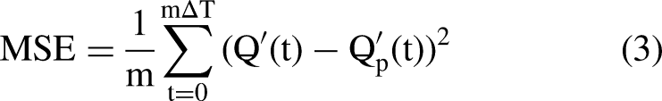$W$ and biases $b$ . The outputs of $i$ th hidden layer are computed as, $Z_{i} = σ (W_{i} Z_{i - 1} + b_{i})$ , where $Z_{i - 1}$ are the outputs of the previous layer and $σ$ indicates activation function. The activation function can be used to introduce nonlinearity to the affine transformation of $W_{i} Z_{i - 1} + b_{i}$ . Therefore, the key design considerations to build a NN model are the number of hidden layers, the number of neurons in each hidden layer, and the activation function to be used. These are called hyper-parameters of the model. Several models with varying hyper-parameters are trained, and the model with the least validation error is selected to predict the flame response. The hyper-parameters considered are: no. of hidden layers, no. of neurons per layer, learning rate and batch size. Table 2 gives the details of the hyper-parameters used. For all the cases considered in this work, we use a NN model with three hidden layers, $[128, 64, 32]$ neurons in each layer respectively. The learning rate and batch size were identified as important hyper-parameters. The grid search²⁸ is performed to exhaustively find the best combination of these values. Learning rate is sampled from ${10^{- 5}, 5 \times 10^{- 5}, 10^{- 4}, 5 \times 10^{- 4}, 10^{- 3}}$ . The batch size is sampled from the range of $[1500, 4500]$ with a step of 50. We explored values of 10, 12 and 15 ms for the history ( $n Δ T$ ) provided to the NN model. No. of hidden layers and no. of neurons are efficiently found using Random search.²⁹ $\tanh$ is used as an activation function. The dropout³⁰ is used as a regularizer and is set to 0.5 for all the hidden layers. The NN model is trained using the Adam optimizer³¹ with a suitable learning rate. The mean squared error (MSE) loss function is used to model the flame response of EM2C burner with unseen back plate temperature. It is given by,

MSE = \frac{1}{m} \sum_{t = 0}^{m Δ T} ({\dot{Q}}^{'} (t) - {\dot{Q}}_{p}^{'} (t))^{2}

(3)

where

m

is the number of data points and

{\dot{Q}}_{p}^{'} (t)

is the heat release rate predicted by the NN model.

ETH burner: Problem formulation

For the ETH burner, NN models are trained using the time series of $u^{'}$ and ${\dot{Q}}^{'}$ . The NN model is trained to solve the following regression problem:

{\dot{Q}}^{'} (t) \approx f (u^{'} (t) | u^{'} (t - Δ t), \dots, u^{'} (t - n Δ t)) \forall t

(4)

The signal’s sampling rate (

Δ T

) is

10^{- 6}

and is increased to

10^{- 5}

for efficient processing by the NN model. The length of the time series is 300 ms. Two datasets of different excitation amplitudes, 0.1 and 1.0, are generated, as shown in Figure 4. We train two NN models, one to predict the linear flame response and another to predict the nonlinear flame response. We will refer to these models as “Model L” and “Model NL,” respectively, throughout the paper. Model L uses data coming from 0.1 excitation amplitude. When trained on only 1.0 amplitude data, Model NL fails to accurately capture the low amplitude response. Therefore, data from 0.1 and 1.0 excitation amplitudes are concatenated to train Model NL. The input and output data are mean normalized using

\bar{u}

and

\bar{\dot{Q}}

, respectively. The velocity data is transformed to include the history of velocity observations as shown in equation (4) and Figure 3. The time series data is divided into the training, validation, and test datasets without shuffling. Table 2 lists the training and test split up used. The training data is divided into the training and validation datasets using

80 : 20

split up. Similar to the EM2C setup, a MLP is used to model the linear and nonlinear flame response of the ETH burner. Table 2 lists the hyper-parameters used to train Model L. The Adam optimizer with the learning rate of

10^{- 5}

is used to train the MLP. The MSE is used as a loss function.

Figure 4.

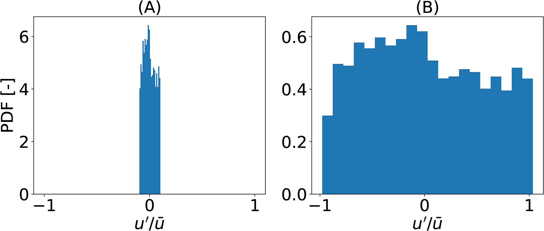
Probability density function of the input velocity signal with (A) 0.1 and (B) 1.0 amplitude fluctuations.

Model NL, which combines the data from two different amplitude levels, provides unsatisfactory results when trained with the MSE loss functions due to the amplitude imbalance problem. The MSE loss function computes the average of the squared differences between the predicted values and the true target values as seen in equation (3). However, the squared term in the loss function can lead to the problem of the model being more sensitive to large errors (associated with larger amplitudes) than to smaller errors (associated with smaller amplitudes). During back-propagation, gradients are scaled by the derivative of the loss function. The gradients can become much larger for larger errors, thus emphasizing the model’s focus on large amplitudes. This can lead the model to prioritize reducing errors for larger amplitudes, which can predict large amplitudes more accurately than smaller ones. To alleviate this issue, we tested different loss functions that do not overly amplify the errors. Such loss functions include mean absolute percentage error (MAPE), normalized MSE, normalized root MSE, and Huber loss. Taking inspiration from these loss functions, we propose a novel loss function that performs best for the underlying data. A novel loss function called mean square root error (MSQRE) is formulated as:

MSQRE = \frac{1}{m} \sum_{t = 0}^{m Δ T} \sqrt{| {\dot{Q}}^{'} (t) - {\dot{Q}}_{p}^{'} (t) |} .

(5)

Results

In this section, we showcase results obtained on two tasks of flame response modelling. First, we assess the model performance on predicting the FTF of a turbulent flame at unseen thermal boundary conditions. Then, we showcase the ability of NN models to capture FTF and FDF of a turbulent flame.

Predicting FTF of a turbulent flame at unseen boundary conditions

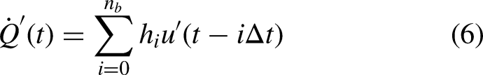
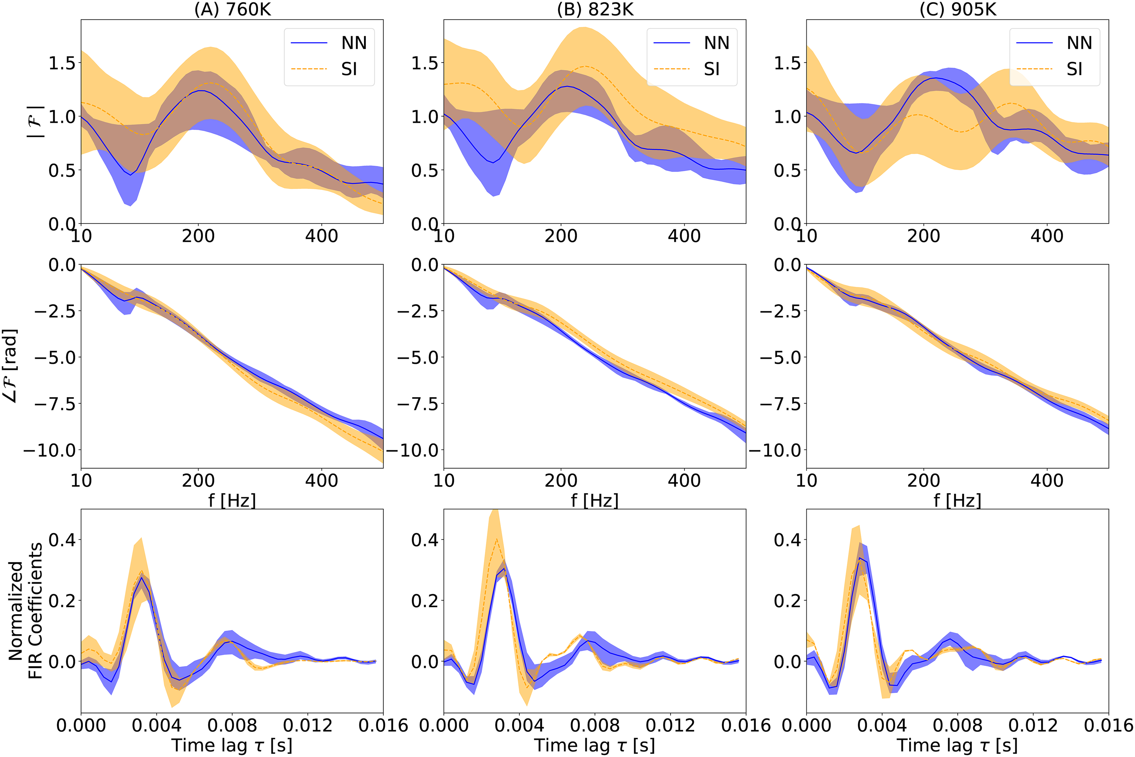
Time series data obtained from 6 LES simulations, at different thermal boundary conditions ( $T_{train}$ ), are used to train the NN model. It is validated on 3 different combustor configurations ( $T_{validation}$ ). The best performing model gives the MSE of $0.0068$ . This trained NN is used to predict FTF of a turbulent flame with unseen back plate temperature ( $T_{test}$ ). To compute the FTF, mono-frequent harmonic excitation signals with 0.1 amplitude are generated in the frequency range from 10 to 500 Hz with 10 Hz resolution. The trained NN model is used to predict the output for each excitation signal. The fast fourier transform is applied to obtain the gain and phase information of the frequency of interest. Figure 5(A) shows the prediction at 760K, which belongs to the test set. The FTF obtained by the NN model is compared against the FTF coming from CFD/SI approach.³² Note that the latter requires data at that temperature: The CFD/SI approach is not capable of evaluating the flame response at unseen conditions. In other words, there is no established method that permits to ‘interpolate’ an impulse response, obtained by the CFD/SI approach, from data obtained at adjacent operating conditions. We observe that the NN model captures the flame response quite accurately. In order to obtain the uncertainty in FTF prediction, we generate multiple realizations of training data using temporal slicing. We slice the input-output time series of 350 ms length into the 5 overlapping time series of length 150 ms each. 5 NN models are trained using these datasets. Additionally, we train a NN model with complete data of 350 ms. The gain and phase predictions obtained from these 6 models are used to calculate upper and lower limits in the FTF prediction. Figures 5(B) and (C) show the prediction bounds of gain and phase obtained by the NN model for additional test cases of 823 and 905 K. Another equivalent approach to comparing the similarity in the predicted flame response is by means of the finite impulse response (FIR) model.^33–35 It describes the effect of an impulse perturbation of velocity on the heat release by the flame. It is formulated as,

{\dot{Q}}^{'} (t) = \sum_{i = 0}^{n_{b}} h_{i} u^{'} (t - i Δ t)

(6)

where

n_{b}

is the number of impulse response coefficients

h_{i}

. The third row of Figure 5 compares the estimated FIR coefficients at three corresponding temperatures obtained by the CFD/SI approach and NN model. The FIR is obtained by performing the inverse z-transform of the calculated FTF. The FIR obtained from the NN model is in good agreement with the CFD/SI approach.

Figure 5.

EM2C burner: Comparison of gain, phase and normalized FIR coefficients of the linear flame response predicted by CFD/SI and NN approach at unseen, interpolated back plate temperatures of (A) 760 K; (B) 823 K; (C) 905 K. The shaded region in blue shows the bounds of prediction by NN model using different realizations of the training data. FIR: finite impulse response; CFD: computational fluid dynamics; SI: system identification; NN: neural network.

In the first two rows of Figure 6, we collect the gain and phase for all 12 configurations using CFD/SI approach and NN model. The phase difference in the resulting NN predictions (Figure 6(B)) displays that increasing the back plate temperature of the EM2C burner results in a decrease in the phase difference. This finding is in good agreement with Kulkarni et al.²⁴ According to that study, higher back plate temperatures cause a reduction in the phase because such high temperatures promote closer stabilization of the flame to the burner mouth and, overall, a shorter flame length. Furthermore, gain curves reveal that increasing back plate temperatures of the EM2C burner shifts the flame response gain to higher frequencies slightly until 250 Hz. In addition, increased back plate temperatures of the EM2C burner amplify the flame response between 250 and 500 Hz.

Figure 6.

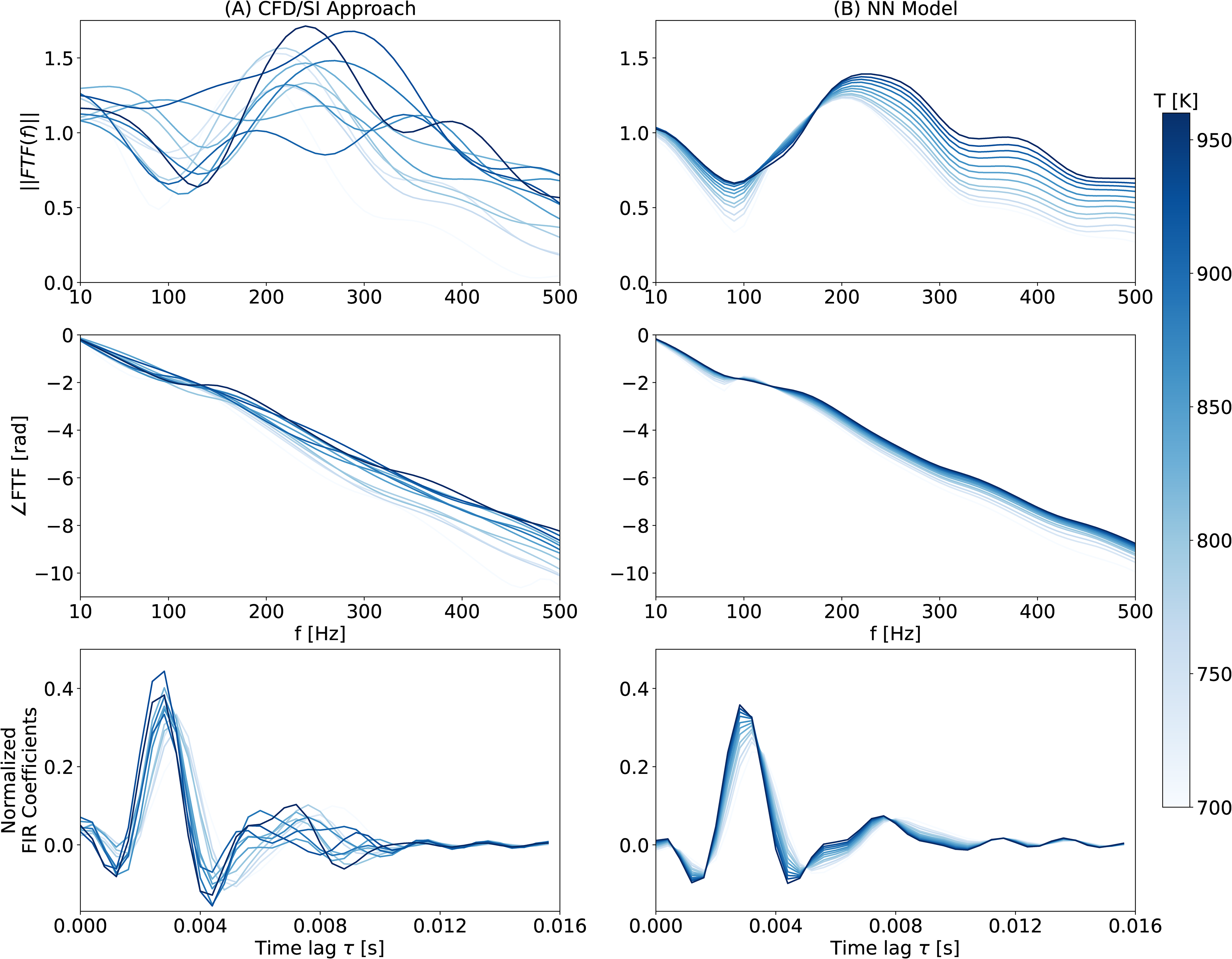
EM2C burner: Comparison between mean gain, phase and normalized FIR coefficients of the linear flame response at 12 different temperatures using CFD/SI and NN technique. CFD: computational fluid dynamics; SI: system identification; NN: neural network; FIR: finite impulse response.

A collection of impulse responses, each of them characterizing the acoustic flame response at a given temperature, is shown in the third row of Figure 6. Each of the shown impulse responses of the NN model are obtained by applying the inverse z-transform to the frequency responses shown in the first two rows of Figure 6. From the results of Figure 6, it is understood that the flame responds faster and stronger for larger temperatures T. Note also that the valleys of the impulse response are also stronger for higher plate temperatures T. This implies that the flame fluctuations – increase and decrease of the integrated flame surface area – are more preponderant in the case of higher T. For smaller plate temperatures T, crests and valleys strength decrease and are shifted to the right (larger times). Similar observations are obtained when looking at the impulse responses obtained by SI, although in this case, the gradual change of the impulse response (when shifting from larger to lower values of T) is not as apparent. The agreement of results between NN and the benchmark case (SI) – second and third row of Figure 6 – demonstrates the validity of NN results when inferring models of the flame response at temperatures that are not present in the training data.

The reader might wonder how to interpret the mistmatch betwen the CFD/SI and NN when looking at the gain of the flame response. Upon studying the first row of Figure 6, it becomes evident that any resemblance between CFD/SI and NN results is challenging to discern. It is important to note that CFD/SI cannot be considered a reference truth, as this technique can be significantly affected by noise, particularly combustion noise present in the data. This effect is especially pronounced in the EM2C burner under investigation, as demonstrated by Kulkarni et al.,²⁴ and reflected in the high uncertainties observed (refer to the top row in Figure 5). Therefore, any comparison of flame response gain between the LES/SI and NN methods must take into account the underlying uncertainties. In contrast, the level of uncertainty is lower when investigating the phase of the flame response and the flame impulse response, allowing for a comparison between the two methods.

Modelling nonlinear flame response

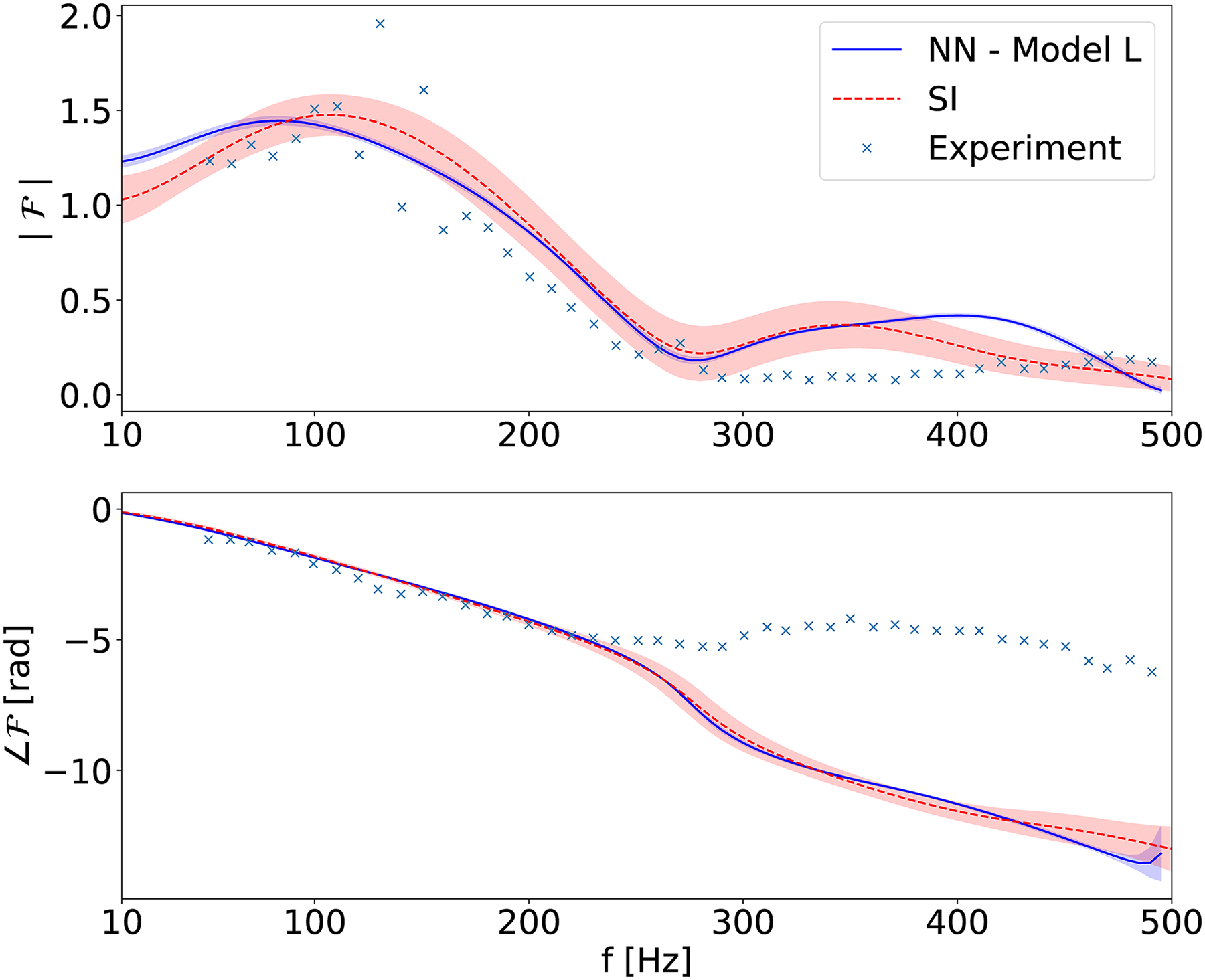
For ETH burner, the time series obtained using a normalized excitation amplitude of 0.1 (Figure 4(A)) is used to model the linear flame response of the flame. 30 $%$ of the data is used for testing and 70 $%$ is used for training. Further, 20 $%$ of the training data is used for validation. A NN model is trained using these time series. The model with the least validation error of $0.0014$ is chosen to further predict the FTF. Hyper-parameters of the selected model are listed in Table 2 and are referred to as Model L. Model L is subjected to mono-frequent forcing at 0.1 amplitude and frequencies in the range of 10 Hz to 500 Hz. Figure 7 compares the FTF obtained by the NN model, CFD/SI method, and experimental data available.³⁶ Overall, a very good agreement is found for the gain and phase prediction done by the NN model with the other data sets.

Figure 7.

ETH burner: Comparison of the FTF predicted by the NN model (Model L) with CFD/SI and experiment. The shaded region in blue shows the bounds of prediction by the top 5 NN models. FTF: flame transfer function; CFD: computational fluid dynamics; SI: system identification; NN: neural network.

Now, we assess the ability of NNs to model the nonlinear flame response. We combine the 0.1 and 1.0 excitation amplitude data to train the NN model. Combining data of 0.1 amplitudes provides NN with more data to train on and improves its prediction at low amplitude levels. This task is more complicated than the FTF prediction due to the variation in gain and phase response to the different amplitudes. First, we study the effect of various loss functions on flame response predictions. Figure 8 compares the FDF predictions by various NN models trained using different loss functions with the LES data coming from mono-frequent excitation. We compare data from 4 different loss functions including the proposed novel loss function. First row shows the gain and phase prediction obtained by NN trained with the MSE loss function. We observe that using the MSE loss function, gains are well-predicted across all amplitude levels but NN is not able to capture the phase separation across various amplitude levels. In contrast to Model L, which was trained with the MSE loss function and able to capture the linear flame response (Figure 7) accurately, the Model NL trained with the MSE loss function is not able to capture the accurate phase for lower amplitudes due to the amplitude imbalance problem. Therefore, we train NN with the MAPE loss function which has the ability to alleviate the amplitude imbalance issue. However, FDF predictions for NN trained with the MAPE are not satisfactory as shown in the second row of Figure 8. Next, we study NN models trained with root mean squared error (RMSE). This loss function helps in improving low amplitude errors due to the square-root in the function. As seen from the third row of Figure 8, it leads to better phase predictions compared to the NN trained with MSE. Therefore, we combine the benefits of these loss functions by proposing a novel loss function MSQRE. We observe that NN models trained with this loss function provide the best performance and therefore, we will discuss these results further in detail.

Figure 8.

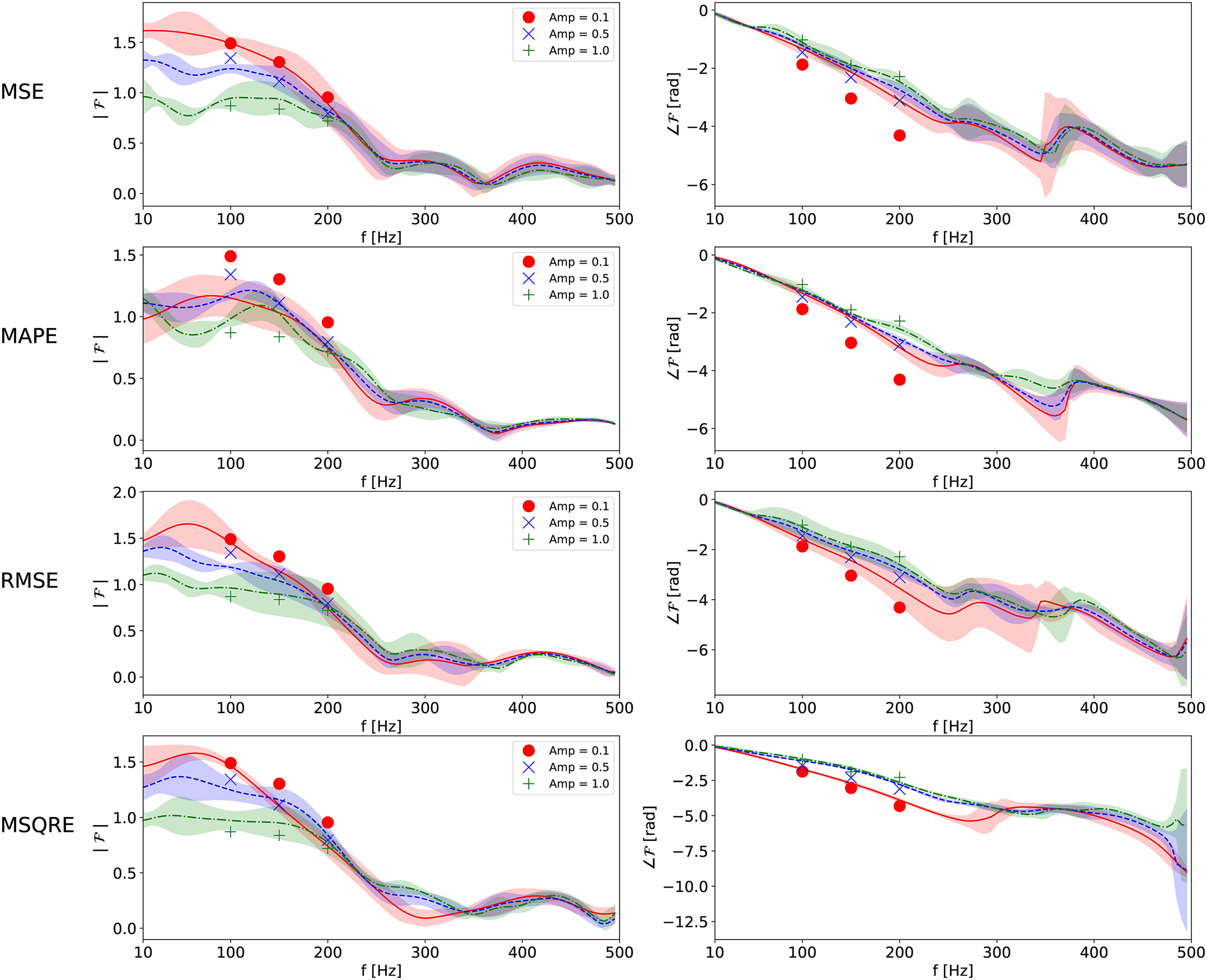
ETH burner: Comparison of effect of various loss functions on FDF prediction by NN model (Model NL) with LES. Solid lines: estimate by the NN model. Markers: ground truth from LES using mono-frequent excitation. The shaded region shows the bounds of prediction by the top 5 NN models. NN: neural network; LES: large eddy simulation; FDF: flame describing function.

The NN models are trained with the novel loss function. The model with the least validation error of 0.2608 is selected to predict the FDF. Figure 9 compares the FDF predicted by the NN model with the data from LES simulations at 0.1, 0.5, and 1.0 amplitude levels. Gains predicted by NN models match accurately with the CFD simulations. A good agreement is observed for the gain predicted by the NN model trained with the MSQRE loss function at 0.1 amplitude level with the CFD/SI approach compared to the NN models trained with MAPE loss function. Similarly, the NN model trained with the MSQRE loss function captures the variation in phase for different amplitude levels of 0.1 and 1.0. The accurate predictions in gain and phase at low amplitude levels stem from the novel MSQRT loss function used to train the NN model. Furthermore, we show the bounds of prediction by selecting the top 5 best-performing NN models from the hyper-parameter study. The predictions by these NN models are used to obtain the mean and standard deviation in gain and phase predictions shown in Figure 9. Therefore, we show that the NN model successfully predicts the linear and nonlinear flame response of the ETH burner under study.

Figure 9.

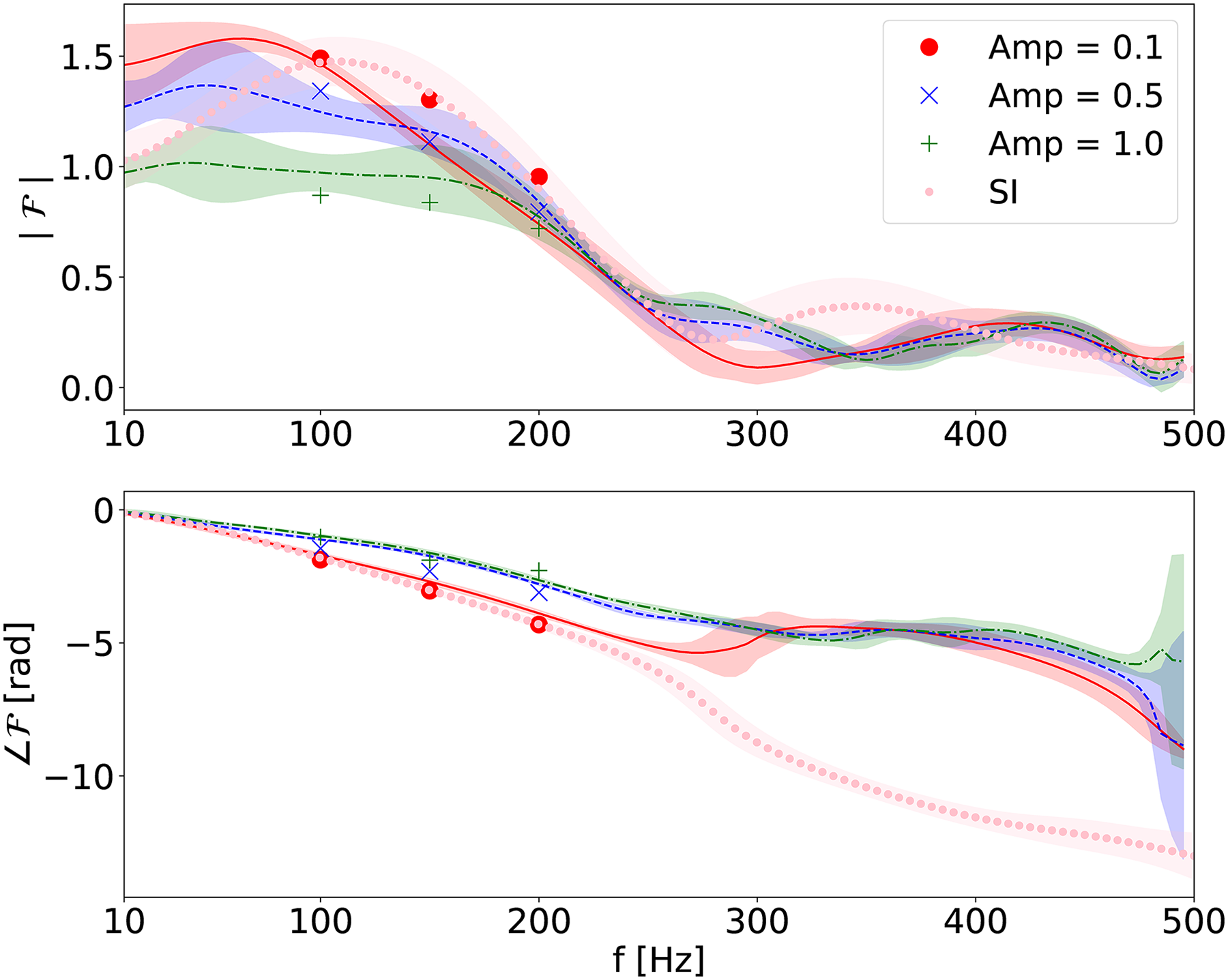
ETH burner: Comparison of the FDF computed from the NN model (Model NL) with LES. Solid lines: estimate by the NN model. Markers: ground truth from LES using mono-frequent excitation. The shaded region shows the bounds of prediction by the top 5 NN models. NN: neural network; LES: large eddy simulation; FDF: flame describing function.

Conclusions and future work

In this work, we demonstrated the ability of the NN model to predict the linear and nonlinear flame response of turbulent flames for two different burner configurations. For the EM2C burner, the NN is trained on the data from a few back plate temperature configurations. The trained NN model can predict the linear flame response at unseen burner configurations with different back plate temperatures. The NN model with sufficient training data can eliminate the need to run additional CFD simulations to capture the FTF at unseen boundary conditions, thus reducing the computational cost. For the ETH burner, the NN model is shown to capture the nonlinear flame response. Compared with the data from the mono-frequent excitations, predictions from the NN model are in good agreement. A novel loss function is shown to be useful to improve flame response predictions.

The present work demonstrates the use of feed-forward NN called MLP to model the linear and nonlinear flame response of turbulent flames. The future works can explore various other NNs such as LSTM to capture temporal relations in the data or Bayesian NN to capture the uncertainties in prediction. Another important direction of future work includes collecting more validation data for ETH case using LES approach for higher frequencies. This effort will contribute to a more comprehensive validation of the NN approach.

Supplemental Material

sj-pdf-1-scd-10.1177_17568277241262641 - Supplemental material for Linear and nonlinear flame response prediction of turbulent flames using neural network models

Supplemental material, sj-pdf-1-scd-10.1177_17568277241262641 for Linear and nonlinear flame response prediction of turbulent flames using neural network models by Nilam Tathawadekar, Alper Ösün, Alexander J. Eder, Camilo F. Silva and Nils Thuerey in International Journal of Spray and Combustion Dynamics

Footnotes

Declaration of conflicting interests

The authors declare no potential conflicts of interest with respect to the research, authorship, and/or publication of this article.

Funding

The authors disclosed receipt of the following financial support for the research, authorship, and/or publication of this article: N. Tathawadekar acknowledges the financial support of the ERC Consolidator Grant SpaTe (CoG-2019-863850) and Alexander J. Eder received financial support from the Deutsche Forschungsgemeinschaft (DFG, German Research Foundation) within the DFG transfer project NoiSI (PO 710/23-1). The authors gratefully acknowledge the Leibniz Supercomputing Centre (LRZ) for funding this project by providing computing time on its Linux-Cluster.

ORCID iDs

Nilam Tathawadekar

Alexander J. Eder

Supplemental material

Supplemental material for this article is available online.

References

Lieuwen

Yang

. Combustion instabilities in gas turbine engines: operational experience, fundamental mechanisms, and modeling. American Institute of Aeronautics and Astronautics, 2005.

Dowling

. Nonlinear self-excited oscillations of a ducted flame. J Fluid Mech 1997; 346: 271–290.

Palies

Durox

Schuller

et al. Nonlinear combustion instability analysis based on the flame describing function applied to turbulent premixed swirling flames. Combust Flame 2011; 158: 1980–1991.

Silva

Nicoud

Schuller

et al. Combining a helmholtz solver with the flame describing function to assess combustion instability in a premixed swirled combustor. Combust Flame 2013; 160: 1743–1754.

Noiray

Durox

Schuller

et al. A unified framework for nonlinear combustion instability analysis based on the flame describing function. J Fluid Mech 2008; 615: 139–167.

Haeringer

Merk

Polifke

. Inclusion of higher harmonics in the flame describing function for predicting limit cycles of self-excited combustion instabilities. Proce Combust Inst 2019; 37: 5255–5262.

Orchini

Juniper

. Flame double input describing function analysis. Combust Flame 2016; 171: 87–102.

Han

Morgans

. Simulation of the flame describing function of a turbulent premixed flame using an open-source les solver. Combust Flame 2015; 162: 1778–1792.

Polifke

Poncet

Paschereit

et al. Reconstruction of acoustic transfer matrices by instationary computational fluid dynamics. J Sound Vib 2001; 245: 483–510.

10.

Hornik

. Approximation capabilities of multilayer feedforward networks. Neural Networks 1991; 4: 251–257.

11.

Raissi

Perdikaris

Karniadakis

. Physics-informed neural networks: A deep learning framework for solving forward and inverse problems involving nonlinear partial differential equations. J Comput Phys 2019; 378: 686–707.

12.

Brand

Yun

et al. Solver-in-the-loop: Learning from differentiable physics to interact with iterative pde-solvers. In Neural Information Processing Systems (NeurIPS), volume 33. pp.6111–6122.

13.

Illarramendi

Bauerheim

Cuenot

. Performance and accuracy assessments of an incompressible fluid solver coupled with a deep convolutional neural network. Data-Centric Eng 2022; 3: e2.

14.

Förner

Polifke

. Nonlinear aeroacoustic characterization of helmholtz resonators with a local-linear neuro-fuzzy network model. J Sound Vib 2017; 407: 170–190.

15.

Jaensch

Polifke

. Uncertainty encountered when modelling self-excited thermoacoustic oscillations with artificial neural networks. Int J Spray Combust Dynam 2017; 9: 367–379.

16.

Kornilov

Rook

ten Thije Boonkkamp

et al. Experimental and numerical investigation of the acoustic response of multi-slit bunsen burners. Combust Flame 2009; 156: 1957–1970.

17.

Rywik

da Cruz

Polifke

. Investigating inconsistent uncertainty quantification encountered in neural network modelling of nonlinear response of a laminar flame. In INTER-NOISE and NOISE-CON Congress and Conference Proceedings, volume 265. Institute of Noise Control Engineering, pp.6199–6207.

18.

Tathawadekar

Doan

NAK

Silva

et al. Modeling of the nonlinear flame response of a bunsen-type flame via multi-layer perceptron. Proce Combust Inst 2021; 38: 6261–6269.

19.

Yadav

Casel

Ghani

. Physics-informed recurrent neural networks for linear and nonlinear flame dynamics. Proce Combust Inst 2022; 39: 1597–1606.

20.

Nicoud

Ducros

. Subgrid-scale stress modelling based on the square of the velocity gradient tensor. Flow Turbul Combust 1999; 62: 183–200.

21.

Colin

Ducros

Veynante

et al. A thickenend flame model for large eddy simulation of turbulent premixed combustion. Phys Fluids 2000; 12: 1843–1863.

22.

Franzelli

Riber

Gicquel

et al. Large eddy simulation of combustion instabilities in a lean partially premixed swirled flame. Combust Flame 2012; 159: 621–637.

23.

Merk

Polifke

Gaudron

et al. Measurement and simulation of combustion noise and dynamics of a confined swirl flame. AIAA J 2018; 56: 1930–1942.

24.

Kulkarni

Guo

Silva

et al. Confidence in flame impulse response estimation from large eddy simulation with uncertain thermal boundary conditions. J Eng Gas Turbine Power 2021; 143: 121002.

25.

Eder

Dharmaputra

Désor

et al. Generation of entropy waves by fully premixed flames in a non-adiabatic combustor with hydrogen enrichment. J Eng Gas Turbine Power 2023; 145: 111001.

26.

Weller

Tabor

Jasak

et al. A tensorial approach to computational continuum mechanics using object-oriented techniques. Comput Phys 1998; 12: 620–631.

27.

Eder

Silva

Haeringer

et al. Incompressible versus compressible large eddy simulation for the identification of premixed flame dynamics. Int J Spray Combust Dynam 2023; 15: 16–32.

28.

Hinton

. A practical guide to training restricted boltzmann machines. Neural Networks: Tricks of the Trade: Second Edition 2012; 599–619.

29.

Bergstra

Bengio

. Random search for hyper-parameter optimization. J Mach Learn Res 2012; 13: 281–305.

30.

Srivastava

Hinton

Krizhevsky

et al. Dropout: a simple way to prevent neural networks from overfitting. J Mach Learn Res 2014; 15: 1929–1958.

31.

Kingma

. Adam: A method for stochastic optimization. Int Conference Learn Representations 2015.

32.

Polifke

. Black-box system identification for reduced order model construction. Ann Nucl Energy 2014; 67: 109–128.

33.

Tangirala

. Principles of system identification: theory and practice. Boca Raton: Crc Press, 2018.

34.

Blumenthal

Subramanian

Sujith

et al. Novel perspectives on the dynamics of premixed flames. Combust Flame 2013; 160: 1215–1224.

35.

Schuermans

Luebcke

Bajusz

et al. Thermoacoustic analysis of gas turbine combustion systems using unsteady CFD. In ASME Turbo Expo 2005: Power for Land, Sea, and Air. American Society of Mechanical Engineers, pp.287–297.

36.

Blondé

. Thermoacoustic Dynamics of Gas Turbine Combustors: Effects of Hydrogen Blending and Tunable Acoustic Boundaries. PhD Thesis, ETH Zurich, Zürich, 2024.

Supplementary Material

Please find the following supplemental material available below.

For Open Access articles published under a Creative Commons License, all supplemental material carries the same license as the article it is associated with.

For non-Open Access articles published, all supplemental material carries a non-exclusive license, and permission requests for re-use of supplemental material or any part of supplemental material shall be sent directly to the copyright owner as specified in the copyright notice associated with the article.

0.00 MB

0.16 MB