Numerical investigation of the response of turbulent swirl non-premixed flames to air flow oscillations

Abstract

The response of swirl non-premixed flames to air flow oscillations is studied using Large-Eddy Simulation (LES) and the Conditional Moment Closure (CMC) combustion model, focusing on the physical mechanisms leading to the heat release rate oscillations observed in a parallel experimental study. Cases relatively close to blow-off and characterized by different amplitude of the flow oscillations are considered. Numerical results are in good agreement with the experiment in terms of both mean flame shape and heat release rate response. Simulations show that the oscillation of the air flow leads to an axial movement and fragmentation of the flame that are more pronounced with increasing amplitude of the forcing. The flame response is characterized by fluctuations of the flame area, time-varying local extinction and lift-off from the fuel injection point. LES-CMC, due to the inherent capability to capture burning state transitions, predicts properly the flame transfer function as a function of the amplitude of the air flow oscillations. This suggests that the response mechanism for this flame is not only due to time-varying flame area, but also local extinction and re-ignition. This study demonstrates that LES-CMC is a useful tool for the analysis of the response of flames of technical interest to large velocity oscillations and for the prediction of the flame transfer function in conditions close to blow-off.

Introduction

Aero-engine combustors often operate in conditions characterized by a high level of unsteadiness where the flame interacts with strong fluctuations of the flow field.^1–4 Flame close to blow-off,^5–7 flame-vortex interactions^1,8,9 and development of combustion instabilities ² are typical examples where the coupling between flame and flow field oscillations is a crucial aspect for the definition of the operability range of the combustor.

Although there is an effort to develop combustion technologies based on premixed lean flames and achieve low emissions through the control of mixture composition, practical aero-engine combustors usually operate with imperfect premixing due to the limited space available for the air-fuel mixing. Most of the combustors currently used in aero-engine applications are still based on a rich primary region,^10,5 followed by quick mixing and lean combustion in the downstream part of the combustor. In addition, pilot stages based on diffusion flames are often used ¹¹ to ensure the stability of the combustor in a wide range of operating conditions. Typical academic studies on flame response to flow field oscillations usually focus on premixed flames,^3,12–15 whereas investigations on configurations characterized by incomplete premixing are more rare (e.g., Refs.^16–19). In order to improve the understanding of the behaviour of flames with different degrees of premixedness, a swirl flame with different fuel injection configurations has been experimentally investigated at University of Cambridge.^20,21 The investigated cases include a fully premixed flame and non-premixed flames with both radial (annular slot) and axial (jet) fuel injection. The study shows significant differences in the flame response to air flow oscillations depending on the fuel injection configuration. In particular, the non-premixed flame characterized by radial fuel injection showed a higher heat release response compared to both premixed flames and non-premixed flames with axial fuel injection. The mechanisms leading to the response of the non-premixed flame with radial fuel injection are investigated in this work using numerical simulations. It is important to point out that this flame was operated relatively close to blow-off with amplitude of the air flow oscillations up to 30% of the flow bulk velocity. Under such conditions, the experiment^20,21 showed an intense flame-flow interaction with the presence of lift-off and possibly local extinction and reignition events.

Numerical simulations have shown a good capability to predict the heat release rate response both in self-excited and forced flames, when approaches able to accurately capture the flow field and turbulence-chemistry interactions are used.^2,22,23 Gathering experimental data on combustion instabilities in real engines is difficult ² and numerical simulations have become a major tool for the analysis of the response of practical combustors.^10,24–26 However, the presence of finite-rate chemistry effects coupled with velocity oscillations makes the flame investigated in this work very challenging to be predicted by numerical simulations. A reliable prediction of the flame response requires the use of models able to accurately capture finite-rate chemistry effects, which imply the use of time-resolved methods for the prediction of the flow and mixing fields together with detailed chemistry and combustion models able to account for the effect of turbulence on the local flame structure. A review of the main models available to predict flame transients, including local extinction and blow-off, is provided by Ref. ²⁷ . In this work, Large-Eddy Simulation (LES) and Conditional Moment Closure (CMC) combustion model are used. The LES-CMC approach has already shown good capability to predict turbulence-chemistry interaction and local extinction in both non-premixed gaseous ²⁸ and spray ²⁹ flames, as well as the full blow-off curve of non-premixed gaseous flames. ³⁰ Therefore, LES-CMC is considered a reliable tool for the investigation of the non-premixed flame studied in Ref. ²⁰ , which is the target of this work. The objectives of this study are to: (i) improve the understanding of the phenomena occurring in the swirl flames with radial fuel injection investigated in Ref. ²⁰ when forcing of the air flow with different amplitudes is applied; (ii) determine the physical mechanisms leading to the heat release rate response observed in the experiment. This study further contributes to assess the capability of the LES-CMC approach to predict the dynamic behaviour of gaseous non-premixed flames characterised by a strong turbulence-chemistry interaction. The paper is organized as follows. First, the configuration and the conditions studied in this work are introduced, followed by a description of the numerical method. Then, results are discussed. Summary and conclusions close the paper.

Configuration

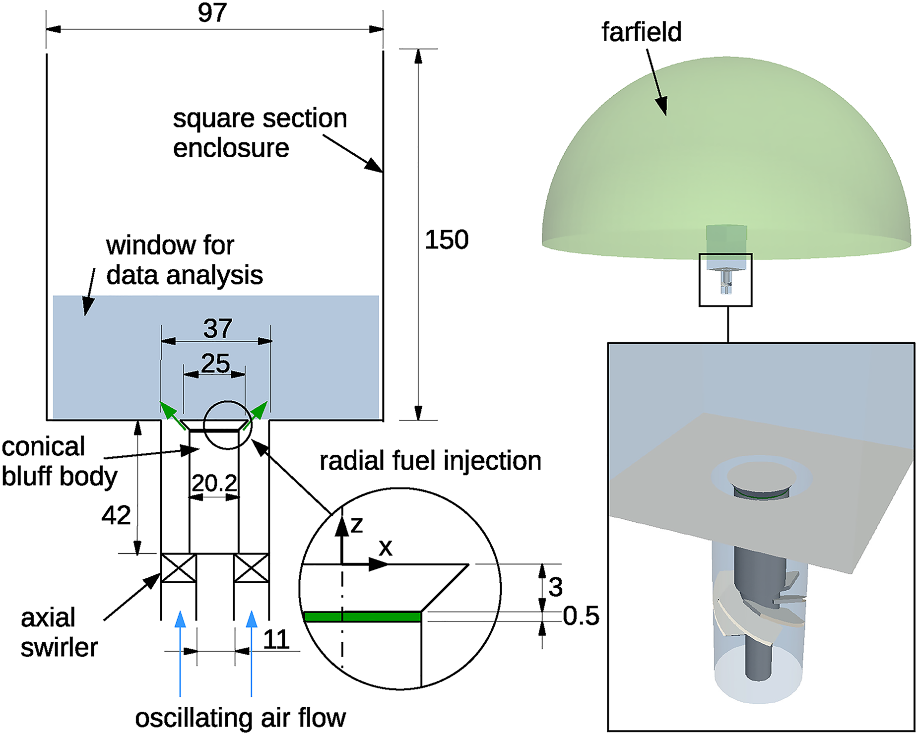
The rig investigated in this work,^21,31 schematically shown in Figure 1, consists of a square section combustion chamber open to the atmosphere at the outlet. Air enters through an annular duct surrounding a conical bluff body with diameter $D=25$  mm. Swirl is imposed by means of a swirler (60 ${}^{\circ }$ vane angle) located upstream of the bluff body. Fuel (methane, $\mathrm{C}{\mathrm{H}}_4$ ) is injected by means of an annular slot located immediately below the conical segment of the bluff body. This configuration allows for an annular distribution of the fuel, which resembles the fuel pattern of typical aero-engine airblast injection systems. Velocity oscillations are imposed to the inlet air by means of two loudspeakers, positioned diametrically opposite each other in an upstream plenum (not shown in Figure 1), as used in Ref. ¹² . The flames are forced at 160 Hz, which is the main resonant frequency of the plenum and burner assembly. ¹² For the sake of data analysis, a frame of reference with origin in the centre of the bluff-body top surface is defined, as shown in Figure 1. The $z$ -axis coincides with the axis of the bluff body, whereas the $x$ -axis is horizontal. Distances will be reported in non-dimensional form using the diameter of the bluff body, $D$ , as reference length scale. For axisymmetric results, the radial coordinate, $r$ , will be used to identify the distance from the axis of the bluff body.

Figure 1.

Schematic of the burner (left) and computational domain (right). All the dimensions are in mm. The Cartesian frame of reference used in the Results section is also shown. The shaded area on the schematic on the left indicates the window analysed in Figures 3 and 5.

Experimental measurements include OH* chemiluminescence, as an approximate indicator of the heat release rate, ²¹ and planar laser-induced fluorescence of OH (OH-PLIF). Comparison between photomultiplier tube and OH* chemiluminescence measurements ³¹ showed that the integrated OH* chemiluminescence signal gives a reliable estimate of the heat release fluctuations in the entire range of investigated conditions. Therefore, OH* chemiluminescence signal was used as a quantitative indicator of heat release rate fluctuations. Furthermore, velocity oscillations at the bluff-body edge were determined from pressure measurements in the upstream plenum by means of the two-microphone technique. ¹² A description of the experimental techniques can be found in Refs.^12,31. The experiment was performed for different air flow bulk velocity, $U_b$ , global equivalence ratio, ${\varphi }_g$ , and amplitudes of the velocity oscillations. Results for a given value of $U_b$ and ${\varphi }_g$ showed an increase of the heat release rate response with increasing amplitude of the velocity oscillation. ³¹ The mechanisms and physical interactions that lead to the response of the flame are investigated in this work through the simulation of three selected cases characterised by the same air flow bulk velocity, $U_b=15.2$ m/s, and global equivalence ratio, ${\varphi }_g=0.55$ , but different amplitude of the velocity oscillation, $A=u_p^{\prime }/U_b$ where $u_p^{\prime }$ is the peak value of the velocity oscillation over the mean at $f=160$ Hz. Cases with $A$ equal to 0 (no forcing), 0.1 and 0.3 are considered in this work. All these cases are relatively close to the flame blow-off ( $U_b/U_{BO}>0.8$ for all the cases, where $U_{BO}$ is the air bulk velocity at blow-off ²¹ ).

Method

LES-CMC

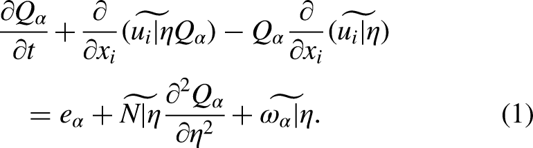
Numerical simulations are performed with the LES-CMC approach ³² , which allows for the computation of the time evolution of the local flame structure (reactive scalars in mixture fraction space), directly taking into account the effect of micro-mixing and turbulent transport. In this work, the same LES-CMC formulation and sub-models described in Refs.^28,30 are used. The mixing field is solved using OpenFOAM, under the low-Mach number assumption. The constant Smagorinsky model is used for the computation of the sub-grid scale stress tensor. A transport equation for the filtered mixture fraction, $\tilde{\xi }$ , is solved, together with equations for mass conservation and momentum balance. The sub-grid scale mixture fraction variance is modelled by an algebraic closure $\widetilde{{\xi }^{″2}}=C_v{\mathrm{\Delta }}^2\mathrm{\nabla }\tilde{\xi }\cdot \mathrm{\nabla }\tilde{\xi }$ , ³³ where $\mathrm{\Delta }$ is the size of the LES filter and $C_v$ is a model constant taken equal to 0.1.^34,28 CMC equations are solved with an in-house unstructured code.^28,35 Following the finite volume implementation adopted here, the CMC equation for the conditionally filtered mass fraction of the $\alpha$ -th species, $Q_{\alpha }=\widetilde{Y_{\alpha }|\eta }$ ( $\eta$ is the mixture fraction sample space variable) can be expressed as ²⁸ :

$$\frac{\mathrm{\partial }{Q}_{\alpha }}{\mathrm{\partial }t}+\frac{\mathrm{\partial }}{\mathrm{\partial }{x}_i}(\widetilde{u_i|\eta }{Q}_{\alpha })-Q_{\alpha }\frac{\mathrm{\partial }}{\mathrm{\partial }{x}_i}(\widetilde{u_i|\eta })=e_{\alpha }+\widetilde{N|\eta }\frac{{\mathrm{\partial }}^2{Q}_{\alpha }}{\mathrm{\partial }{\eta }^2}+\widetilde{{\omega }_{\alpha }|\eta }.$$

(1)

The term $e_{\alpha }$ represents the sub-grid scale turbulent transport, modelled with the typical gradient assumption. ²⁸ The conditionally filtered velocity, $\widetilde{u_i|\eta }$ , is modelled as $\widetilde{u_i|\eta }=\widetilde{u_i}$ , whereas the conditionally filtered scalar dissipation rate, $\widetilde{N|\eta }$ , is closed by the Amplitude Mapping Closure model ³⁶ : $\widetilde{N|\eta }=N_{0}G(\eta )$ , with $G(\eta )=\exp (-2[{\mathrm{erf}}^{-1}(2\eta -1){]}^2)$ and $N_0=\tilde{N}/{\int }_0^1\tilde{P}(\eta )G(\eta )d\eta$ . $\tilde{N}$ is the mixture fraction scalar dissipation rate which consists of contributions from both the resolved and sub-grid scales: $\tilde{N}=D\mathrm{\nabla }\tilde{\xi }\cdot \mathrm{\nabla }\tilde{\xi }+0.5C_N{\mu }_{sgs}\widetilde{{\xi }^{″2}}/(\overline{\rho }{\mathrm{\Delta }}^2)$ , where $D$ is the molecular diffusivity, ${\mu }_{sgs}$ is the sub-grid scale turbulent viscosity, $\overline{\rho }$ is the filtered density and $C_N$ is a model constant taken equal to 42.0.^37,28,38 The conditionally filtered chemical source term, $\widetilde{{\omega }_{\alpha }|\eta }$ , is closed with a first order approximation. The ARM2 mechanism ³⁹ (19 species and 15 reactions) is used. An equation similar to Eq. 1, without the chemical source term, is solved for the conditionally filtered enthalpy. Unconditional filtered values are obtained from the CMC solution through integration over the mixture fraction Filtered probability Density Function (FDF), $\tilde{P}(\eta )$ , modelled with a presumed $\beta$ -function shape computed from the filtered mixture fraction and its sub-grid scale variance. It should be noted that previous work using the same method (LES-CMC models and chemical mechanism) has shown that this framework can predict quantitatively ignition and flame propagation, ⁴⁰ local extinctions and re-ignitions, ²⁸ as well as global blow-off of methane flames. ³⁰ Based on the validation done in previous work, the LES-CMC method used in this study can be considered a reliable framework to develop further understanding on the flow-chemistry interactions that characterise the forced response of a methane burner operated in conditions relatively close to blow-off.

Numerical Setup

The computational domain, schematically shown in Figure 1, reproduces the experimental rig and includes the axial swirler upstream of the bluff-body and a plenum in the farfield. The LES equations are solved in a fully tetrahedral mesh of about 22.4 million cells. Local refinements have been used in the flame region and in the upstream duct to properly capture the flame dynamics and turbulent structures that develop in the annular duct. The maximum LES filter size in the reacting region is about 0.4 mm. Tests showed that the resolution adopted here is sufficient to resolve at least 85% of the turbulence kinetic energy in the entire combustion chamber. Following common practice,^28,30 the CMC equations are solved in a coarser mesh. A CMC grid of about 135,000 cells is used. This mesh, obtained by clustering LES cells, ³⁰ has been refined in the flame region and also upstream of the bluff body, inside the annular duct, where high gradients of mixture fraction are expected. The transfer of quantities from the LES to the CMC resolution is based on a FDF-weighted average. ²⁸ Spatially uniform velocity is imposed at the inlet of the domain. For the forced cases, velocity oscillations are imposed through a sinusoidally time-varying mass flow rate ${\dot{m}}_{air}(t)={\dot{m}}_{b,air}[1+A\sin (2\pi ft)]$ , where ${\dot{m}}_{b,air}$ is the mass flow rate based on the bulk velocity and $f$ is the frequency of the forcing. Constant flow rate was used for the fuel inlet. No-slip adiabatic condition is used for all the solid boundaries. Constant pressure, equal to 1 atm, is imposed at the farfield outlet whereas a low velocity air co-flow is imposed at the base of the farfield, to improve the numerical stability of the computations. The mixture fraction space is discretized by means of 51 nodes, clustered around the stoichiometric mixture fraction ( ${\eta }_{st}\approx 0.055$ ). Pure air is imposed at $\eta =0$ , whereas pure fuel is imposed at $\eta =1$ . Ambient temperature, equal to 298 K, is used for both boundaries. A zero-gradient condition is used at the outlet and solid walls for the CMC equations. The inert mixing solution is imposed both at the air and fuel inlets. Simulations are performed with a time step equal to 1  $\mu \mathrm{s}$ for both the LES and CMC solvers. Second-order accurate numerical schemes, both in space and time, are used in the LES. An operator splitting technique ²⁸ is used for the solution of the CMC equations with chemistry integration performed using the VODPK solver, ⁴¹ as detailed in Ref. ²⁸ . Statistics are collected over 8 periods of the forcing oscillation, corresponding to about 5 flow-through times of the burner. The simulations were performed on 480 2.7 GHz cores (E5-2697 v2 -Ivy Bridge) with 2.6 GB of RAM per core. The computation of 1 ms of physical time requires almost 8 h.

Results and Discussion

Mean flame shape

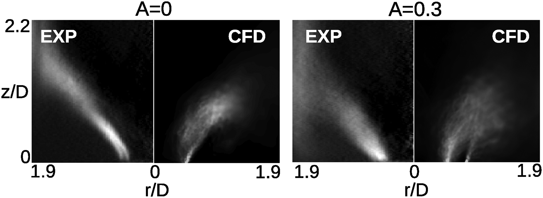
The mean flame shape is revealed in the experiment by the time-averaged OH* chemiluminescence and OH-PLIF measurements. Figure 2 shows a comparison between the inverse Abel-transformed mean OH* chemiluminescence signal and the mean heat release rate (HRR) predicted by the simulation for the case without forcing, $A=0$ , and the forced case with $A=0.3$ . The experiment shows that the flame is characterized by a region of high heat release rate along the air flow shear layer. This region seems located along the inner shear layer in the case without forcing and becomes wider as velocity oscillations are introduced, suggesting a higher dispersion of the location of the flame front. Furthermore, regions with high mean heat release rate also appear close to the wall. The simulation is able to predict reasonably well both the region with high HRR along the air shear layer and the increase of the spatial dispersion of the HRR due to the presence of the forcing. Simulations also indicate the presence of heat release on the outer shear layer of the air flow when the forcing is imposed. Although simulations show heat release rate at the wall (see also Figure 6), the relative intensity between the HRR in this region and the HRR along the air shear layer appears underpredicted in the simulation compared to the experiment. This might be due to an underestimation of the scalar dissipation rate in the region close to the wall and will be further investigated in future work. However, as further discussed in a following section, the impingement of the flame on the wall has only a minor effect on the global heat release response, therefore making the study performed here relevant for the characterization of the flame response. Figure 3 shows comparisons between the mean OH-PLIF signal and mean OH mass fraction predicted by the simulation for the case without forcing and for the case with $A=0.3$ . As the forcing is introduced, the experiment shows that the OH-containing region becomes more dispersed with high levels of OH along the burner centreline and in the outer recirculation zones. Numerical results show a slightly higher dispersion of the OH-containing region along the inner shear layer. However, the location of the OH-containing regions with and without forcing as well as the location of flame impingement on the wall are well predicted.

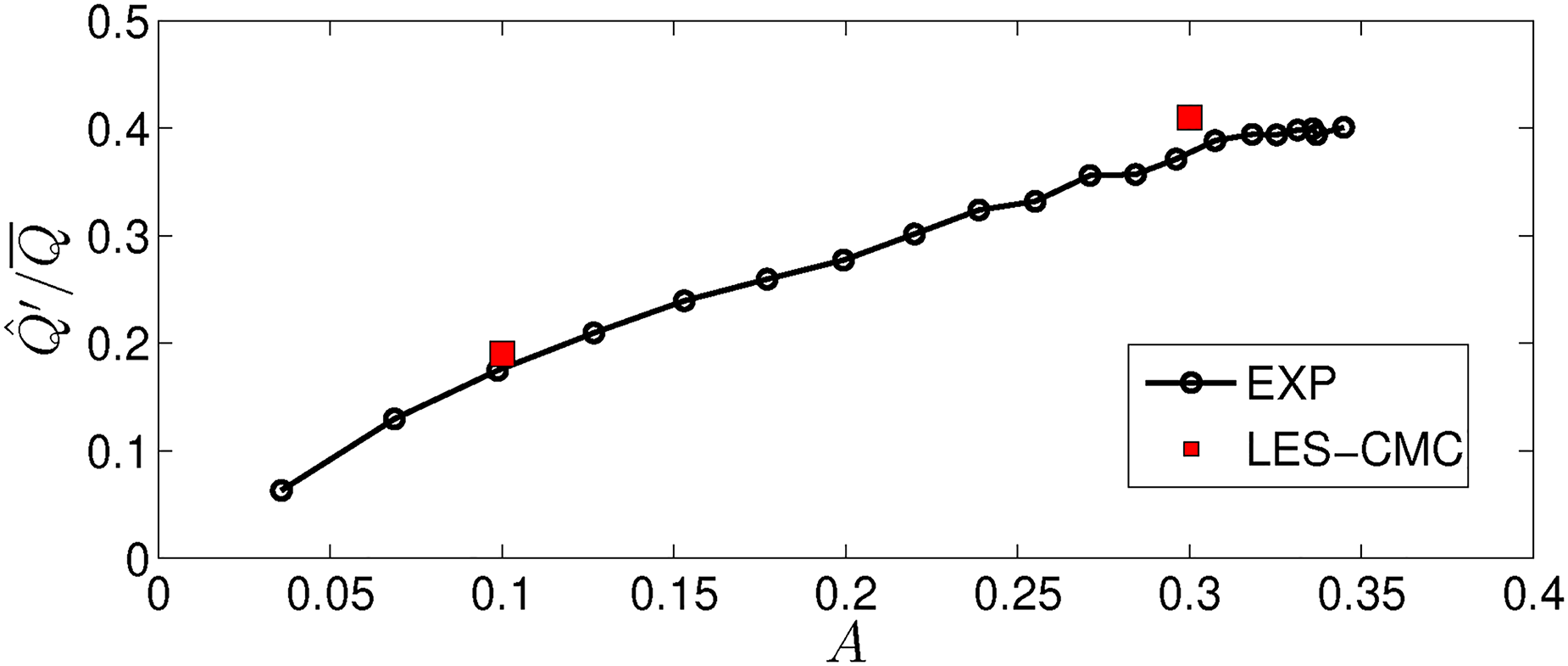
The heat release response of the forced flames was evaluated through the analysis of the time evolution of the volume-integral of the HRR (OH* signal in the experiment) in the flame region. Forced flames exhibit a strong fluctuation of the integrated HRR at the forcing frequency, with the amplitude of the fluctuation that increases with increasing amplitude of the velocity oscillations. The non-dimensional HRR response, $\widehat{Q^{\prime }}/\overline{Q}$ where $\widehat{Q^{\prime }}$ is the amplitude of the HRR fluctuations at the forcing frequency and $\overline{Q}$ is the mean (volume-integrated) HRR, is shown in Figure 4. Note that $\overline{Q}$ and related heat release rate fluctuations are computed for each case independently, using the respective time series. However, since the fuel flow rate is the same in all cases, no significant differences between the mean heat release rate of the various cases are expected. This is confirmed by the numerical simulations, which predict variations of the mean heat release rate within 5% of the value found for the unforced case. The numerical simulation predicts well both the level and the trend of the HRR response for different amplitudes of the velocity oscillations. Therefore, the capability of numerical simulations to predict the response of the flame to velocity oscillations, already shown for premixed flames (e.g., Refs^22,23), is further demonstrated in the context of non-premixed flames in conditions close to blow-off. The physical mechanism leading to the flame response is discussed next.

Figure 2.

Comparison between inverse Abel-transformed mean OH* chemiluminescence signal from the experiment ²¹ and mean heat release rate from the LES-CMC for $A=0$ (no forcing) and $A=0.3$ .

Figure 3.

Comparison between mean OH-PLIF signal from the experiment ²¹ and mean OH mass fraction predicted by the LES-CMC for $A=0$ (no forcing) and $A=0.3$ .

Figure 4.

Non-dimensional heat release rate fluctuations at the forcing frequency as a function of the amplitude of the velocity oscillation: comparison between experiment ³¹ and numerical simulation.

Figure 5.

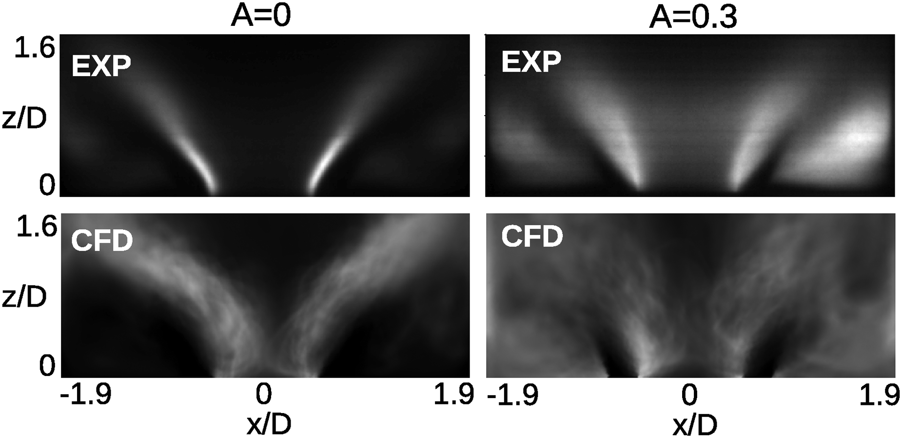
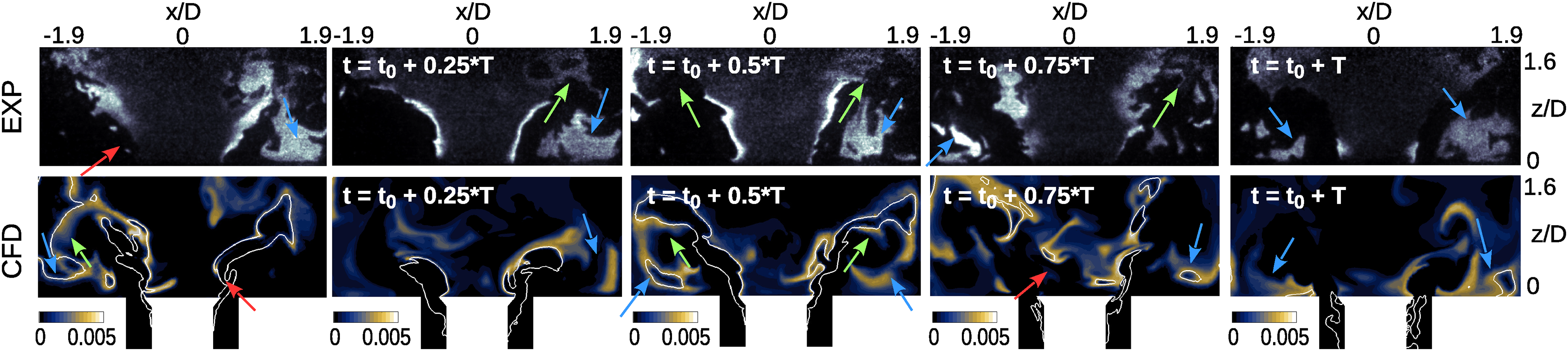
Comparison between instantaneous OH-PLIF images from the experiment ²¹ (top row) and instantaneous OH mass fraction from the LES-CMC (bottom row) for the forced case with $A=0.3$ . The white line indicates the stoichiometric mixture fraction. Red arrows indicate occasional flame lift-off; blue arrows indicate OH in the corner recirculation region; green arrows point the rounded shape of the flame.

Figure 6.

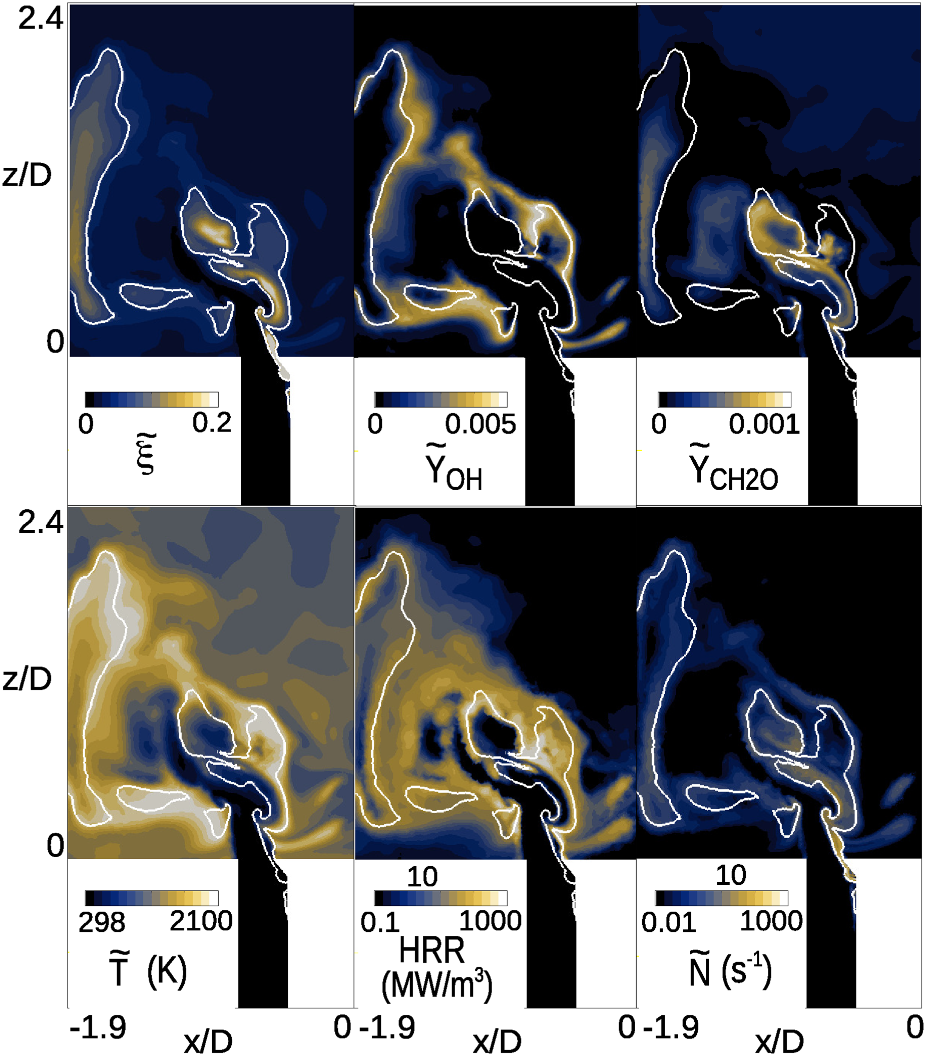
Instantaneous unconditional filtered quantities in a streamwise cross section (forced case, $A=0.3$ ). The white iso-line is the stoichiometric mixture fraction.

Flame dynamics

The instantaneous flame shape with the presence of forcing ( $A=0.3$ ) is shown in Figure 5 where OH-PLIF images at selected time instants during a period, $T=6.25$ ms, of the forcing are compared with instantaneous snapshots of resolved OH mass fraction from the LES-CMC computation. The experiment shows a strong dynamic behaviour of the flame. OH-containing regions are generally located along the inner shear layer of the air flow and develop downstream, sometimes showing a rounded shape as indicated by green arrows. During the forcing cycle, occasional lift-off at the bluff body edge is observed (red arrows) as well as impingement of the OH containing regions on the wall. Pockets of OH can be trapped in the corner recirculation zone (blue arrows), where extended regions with presence of OH are often observed during the cycle, leading to the high OH concentration observed in the mean image (Figure 3). During part of the cycle, the OH-containing region along the inner shear layer can be completely destroyed and only isolated pockets are present. All these features are properly captured by the numerical simulation. The location of the isoline of the stoichiometric mixture fraction, ${\tilde{\xi }}_{st}$ , shows high levels of fluctuations in the axial direction. These fluctuations can be correlated with the fluctuations of the air velocity (see also the discussion of the flame response mechanism in a following section). Rich mixture develops from the injection location and penetrates downstream of the bluff-body edge leading to a conical flame shape. However, during part of the cycle it is evident that the ${\tilde{\xi }}_{st}$ isoline can completely retract inside the annular duct, with only residual pockets of OH appearing in the combustion chamber. Note that when the ${\tilde{\xi }}_{st}$ isoline penetrates in the flame region, only the inner branch of the stoichiometric region shows presence of OH mass fraction, consistent with the experiment.

The flame structure when stoichiometric mixture penetrates into the flame region is further investigated in Figure 6 where selected flow field quantities and species mass fractions at a given time instant are shown. $\tilde{\xi }$ is the resolved mixture fraction whereas $\tilde{N}$ is the scalar dissipation rate with contributions both from the resolved and sub-grid scales. ²⁸ The outer branch of stoichiometric mixture, located inside the annular gap, is characterized by low temperature and absence of OH and HRR, indicating quenching of the flame in that region. Inspection of the CMC solution indicates that the extinction is due to a combination of micro-mixing effects, as also suggested by the relatively high value of scalar dissipation rate (see Figure 6), and transport of inert mixture from the inlet. Further downstream, the mixture ignites leading to a rounded shape of the OH-containing region also observed in the experiment. Stoichiometric mixture can impinge on the wall, where heat release rate is observed as in the experiment. Isolated pockets of rich mixture can enter the corner recirculation region where the subsequent mixing leads to a wider distribution of the OH mass fraction, consistent with the experiment. Pockets of rich mixture trapped in the corner recirculation zone might reach the outer shear layer of the air flow, causing the presence of relatively high HRR in that region. High scalar dissipation rate can occasionally lead to local extinction also along the inner branch of the stoichiometric mixture causing lift-off of the flame (see red arrow in Figure 5, left). However, lift-off might also be due to the absence of fuel during the transient that brings to the retraction of the rich mixture in the upstream duct (see the red arrow in Figure 5, right).

Flame response mechanism

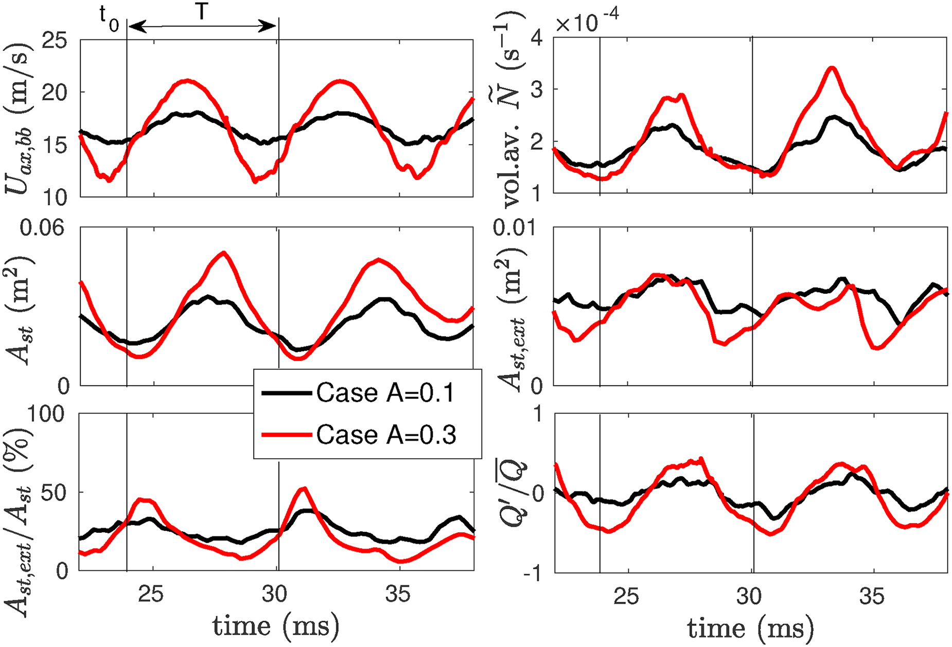
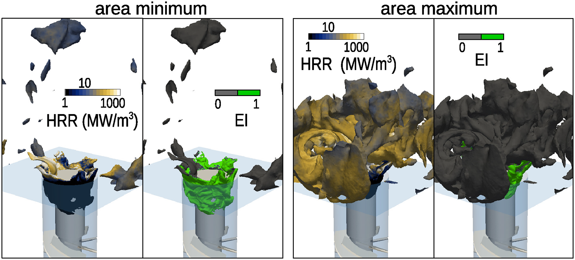
The mechanism leading to the flame response observed in both experiments and numerical simulations is further analysed through Figure 7 where the time evolution of the axial velocity at the bluff-body edge (averaged value) is shown for the two forced cases investigated in this work, together with the area of the stoichiometric iso-surface $A_{st}$ (which gives an indication of the flame surface), volume-averaged scalar dissipation rate, and volume integral of heat release rate. The area of the ${\tilde{\xi }}_{st}$ iso-surface characterized by local extinction, $A_{st,ext}$ , is also estimated as the area with OH mass fraction lower than ${10}^{-4}$ . This threshold value corresponds to about $5$ % of the OH mass fraction at stoichiometry computed by a 0D-CMC computation (i.e., stand-alone solution of the CMC equations without terms representing transport in physical space) at the critical scalar dissipation rate. ²⁸ Figure 7 shows that the increase of the air flow velocity generally leads to an increase of the flame surface area, with the peak of the area lagging the peak of velocity. The HRR response is well correlated with the increase of flame area. The extinguished area generally increases with increasing air velocity, suggesting that higher $\tilde{N}$ caused by the higher velocity might increase the amount of local extinctions. This is also partly indicated by the behaviour of the volume-averaged scalar dissipation rate which shows peaks in correspondence of peaks of velocity and heat release rate. This increase of the volume-averaged scalar dissipation rate should be related to higher mixture fraction gradients at parts of the cycle. However, as revealed by the ratio $A_{st,ext}/A_{st}$ , it is important to note that when the flame surface shows minima, as much as 40–50% of the ${\tilde{\xi }}_{st}$ isosurface is extinguished. This is further highlighted in Figure 8 where the stoichiometric mixture fraction iso-surface at two selected instants, characterized by a minimum and maximum of the flame area respectively, is shown for the case characterized by the larger velocity oscillations ( $A=0.3$ ). The stoichiometric mixture located upstream of the bluff body edge is generally extinguished, as indicated by the negligible value of HRR. To better visualise the extinguished areas, an extinction index, EI, has also been introduced. EI is equal to 1 in the region with OH lower than the threshold value. On the contrary, EI $=0$ indicates regions with values of OH above the threshold. Results for the flame at a maximum and a minimum of the flame surface are included in Figure 8. When the flame surface has a minimum, most of the stoichiometric area consists of mixture retracting in the annual duct, with residuals of reacting regions represented by isolated pockets of stoichiometric mixture with various dimensions. It should also be noted that the response of the flame discussed here in terms of integral values is the result of a number of unsteady phenomena, which characterise the local flame structure and are driven by interactions with the flow field. As already discussed through the instantaneous snapshots of Figure 5 (the corresponding time period is also shown in Figure 7 for reference), local extinctions, retraction of stoichiometric mixture upstream of the bluff body edge, fragmentation of the flame and re-ignition phenomena contribute to the overall behaviour of the flame. It is interesting to note that the minimum of the stoichiometric iso-surface area is given by the combination of upstream movement of the mixture and the dilution of the residual mixture in the flame region. The latter is the main responsible for the delay of the minimum of $A_{st}$ compared to the minimum of the bulk velocity at the bluff-body edge. Stoichiometric mixture introduced back into the flame region is usually not burning. Re-ignition dynamics and turbulence-chemistry interactions eventually determine the heat release-response. It is evident that only a combustion model that included local extinctions would predict $A_{st,ext}/A_{st}>0$ , which seems to be an important mechanism to explain the overall HRR in this flame.

Figure 7.

Axial velocity at the bluff-body edge, volume-averaged scalar dissipation rate, stoichiometric surface area, extinguished area, area extinction ratio, and heat release rate predicted by the LES-CMC simulation for the two forced cases investigated in this work. The time period corresponding to the analysis of selected snapshots reported in Figure 5 is also marked.

Figure 8.

Stoichiometric mixture fraction isosurface coloured with heat release rate (HRR) and extinction index (EI) at two selected time instants for the forced case with $A=0.3$ . Left: flame area minimum; Right: flame area maximum.

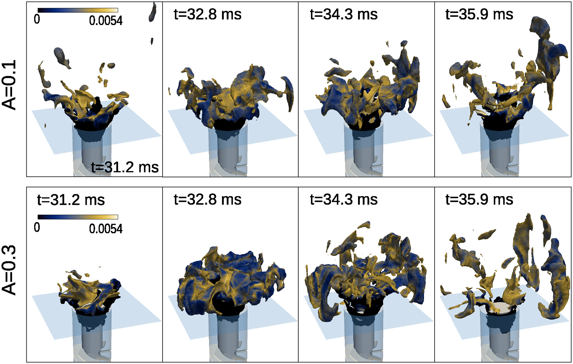
The flame dynamics during a forcing cycle is further analysed in Figure 9 through the time evolution of the ${\tilde{\xi }}_{st}$ iso-surface during one cycle of the forcing. The larger variations of the flame surface area in the case with $A=0.3$ compared to the case with $A=0.1$ are evident, as well as the more intense axial movement of the flame and the higher fragmentation induced by the swirling flow. Note that in the case with $A=0.3$ the ${\tilde{\xi }}_{st}$ iso-surface completely retracts in the upstream duct, with only isolated reacting regions left in the domain, whereas for less intense velocity oscillations the flame keeps the annular structure for the entire cycle. As also shown in Figure 7, an increase of the amplitude of the velocity oscillations leads to higher fluctuations of the flame surface area and scalar dissipation rate. These oscillations are also correlated with local extinctions and re-ignition events. Therefore, the increase of the heat-release rate fluctuations with increasing amplitude of the air flow oscillations observed in the experiment (see Figure 4) can be attributed to the combination of variations of flame surface area and turbulence-chemistry interactions (flame fragmentation and local extinctions) induced by variations of the velocity and mixing fields.

Figure 9.

Flame response over one forcing period predicted by the LES-CMC and visualized through the isosurface of the stoichiometric mixture fraction coloured with OH mass fraction. Top row: $A=0.1$ ; Bottom row: $A=0.3$ .

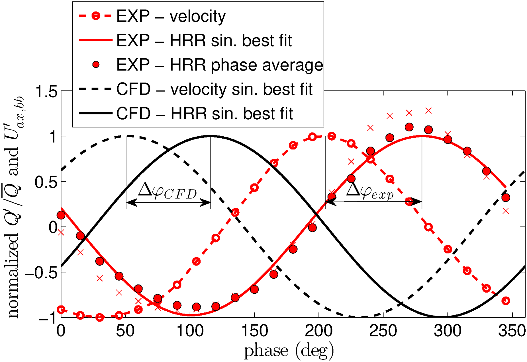
An additional quantity to analyse is the phase shift between the velocity and heat release rate oscillations. A comparison between the experiment and the numerical simulation for the forced case at $A=0.3$ is given in Figure 10. Phase average was used in the experiment whereas the numerical prediction was obtained through a best sinusoidal fitting applied to the collected data (similar phase shift results were obtained by means of the correlation of the two signals). The comparison shows a good agreement between experiment ( $\mathrm{\Delta }{\phi }_{exp}\approx {74}^{\circ }$ ) and numerical simulation ( $\mathrm{\Delta }{\phi }_{CFD}\approx {65}^{\circ }$ ), with the phase shift slightly underpredicted by the simulation (note that the relative phase between experiment and simulation is only due to the reference signal used in the post-process). Post-process of the experimental data was also performed without considering the region close to the walls (25 mm on both sides) and results are indicated by crosses in Figure 10. Results are consistent with the ones obtained considering the entire heat release rate response, both in terms of phase and amplitude of the oscillations. This suggests that the wall behaviour is not crucial in determining the response of the flame, further highlighting the reliability of the flame response mechanism suggested here.

Figure 10.

Phase shift between the velocity oscillation at the bluff-body exit and heat release rate oscillations (forced case, $A=0.3$ ): comparison between experiment and numerical simulations. Crosses indicate experimental phase-averaged values obtained without considering the wall region in the post-process.

Summary and Conclusions

The forced behaviour of a swirl non-premixed methane flame, relatively close to blow-off, has been investigated using numerical simulations based on the LES-CMC approach. The flame response for different amplitudes of the velocity oscillations has been analysed, hence improving the understanding of the physical phenomena leading to the heat release oscillations observed in the experiment.

Finite-rate chemistry and turbulence transport effects appear key elements for the prediction of the flame response, which is characterized by flame lift-off and extended regions with local quenching. The mechanism leading to fluctuations of the heat release rate can be described in terms of fluctuations of the flame surface area due to the axial movement of the flame induced by the air flow oscillations. In case of large oscillations, the stoichiometric mixture may completely retract in the upstream duct where the flame is extinguished, making the subsequent re-ignition inside the combustion chamber crucial for a correct prediction of the global heat release response.

The good agreement between numerical simulations and experiment, both in terms of mean flame shape and dynamic response of the reacting region, shows a promising degree of maturity of the LES-CMC approach to predict the heat release response to large velocity oscillations in flames relevant to gas-turbine applications.