Sage Journals: Discover world-class research

Abstract

The lower limb exoskeleton robot is capable of providing assisted walking and enhancing exercise ability of humans. The coupling human–machine model has attracted a lot of research efforts to solve the complex dynamics and nonlinearity within the system. This study focuses on an approach of gait trajectory optimization of lower limb exoskeleton coupled with human through genetic algorithm. The human–machine coupling system is studied in this article through multibody virtual simulation environment. Planning of the motion trajectory is carried out by the genetic algorithm, which is iteratively generated under optimization of a set of specially designed fitness functions. Human motion captured data are used to guide the evolution of gait trajectory generation method based on genetic algorithm. Experiments are carried out using the MATLAB/Simulink Multibody physical simulation engine and genetic algorithm-toolbox to generate a more natural gait trajectory, the results show that the proposed gait trajectory generation method can provide an anthropomorphic gait for lower limb exoskeleton device.

Keywords

Lower limb exoskeleton human–machine coupling genetic algorithm simulation

Introduction

The study of exoskeleton robots dates to the 1960s.¹ The original research purpose is mainly to improve the carrying capacity of soldiers. With the continuous development of robotics and bio-detection technology, the research of exoskeleton robots has made a breakthrough and some products have been commercialized.^2

–7 As a wearable device that combines human intelligence with the robotic power of robots, its unique human–machine integrated control and design has attracted widespread attention from researchers all over the world. Among the exoskeletons, the lower limb exoskeleton (LLE) robot can provide assisted walking or enhancing exercise ability, which has become an important branch in the field of exoskeleton research. The LLE can be divided into three categories according to the scope of application. The first application focuses on gait rehabilitation, such as Lokomat,⁵ ALEX,⁸ and Ekso GT.⁹ The second application is human locomotion assistance for those paralyzed patients with locomotion handicaps, such as ReWalk¹⁰ and Vanderbilt.¹¹ The third application of LEEs is aimed at enhancing the physical abilities of normal humans, BLEEX,^12,13 HAL-5,¹⁴ and HEXAR,¹⁵ are well known by their augmentation capabilities.

The LLE robot is a typical application of the human–machine coupling system, and the construction of its analytical model is a very complex challenge. Usually, it is necessary to establish a kinematic and dynamic model of a robot system. Denavit–Hartenberg (DH) parameter method^16,17 is a popular way to describe the relationship between components in a robot system when analyzing the forward and inverse kinematic. The main idea of this DH method expresses the position and attitude of the target object in the same coordinate system by vector operation. Despite the kinematic modeling, Kane’s method¹⁷ and Lagrange’s method¹⁸ usually used for analyzing the differential equations of system’s dynamic problem, which play an important role in designing real robot systems. However, as the increasing of complexity and the number of components in the robot system, it increases the complexity to analyze the LLE system using these mathematical modeling methods. With the development of computer-aided design tools and virtual prototype modeling technics, physics-based modeling¹⁹ is gradually becoming a common and efficient method during the system parameters modeling and optimization. Geijtenbeek et al.²⁰ present a musculoskeletal system for simulating bipeds in which both the muscle routing and control parameters are optimized using Open Dynamics Engine (ODE)²¹ simulation environment. In the same software, Heinen et al.^22,23 create a system for legged robot study named LegGen. Aliman et al.²⁴ proposed an LLE structure coupled with human model by combining CATIA (mechanic design) and ADAMS (dynamic simulation). In the studies of the literature,²⁵ a biped robot simulation with several different configurations is established in MATLAB. Compared with the mathematic methods,¹⁶ physics-based methods²⁰ can get rid of the matters caused by complex mathematic differential equations. Moreover, in the process of designing real electromechanical systems, a physics-based method provides researchers with tremendous design creativity and flexibility. In addition to geometric modeling, kinematics and dynamics simulation, physics-based method can be used for us before actual manufacturing which provides great design creativity and flexibility, greatly reducing costs of time and money. The human–machine coupling system proposed in this article is inspired from the previous research.

On the other hand, another major challenge in designing LLEs is walking trajectory generation. There are various methods for planning walking patterns, depending on the application and structure of the exoskeleton.²⁶ These methods can be classified into off-line, online, and a combination of both. The off-line trajectory method mainly includes using mathematical expression^16,27 and recorded human motion data.²⁸ Like the biped robots, zero-moment-point method¹⁶ are used as stability criteria. In Biagiotti and Melchiorri,²⁹ the study shows that the planned gait trajectory is much like the physiological gait trajectory of healthy humans. Online mode relies on sensors that extract user intention to trigger the proper exoskeleton movement, the sensors can be biomechanical (e.g. accelerometer, inertial sensor, and gyro sensor) or bioelectrical (e.g. electromyogram (EMG) and electroencephalogram (EEG)). But a well-designed online trajectory generates methods that demand the accuracy of sensors strongly. With the development of intelligent algorithms, more advanced methods have been proposed in optimizing gait trajectory recently. In Gomes et al.,³⁰ the researchers improved the parameters of neural oscillators to generate joint trajectories. This work with an optimizing system developed to find optimal parameter of neural network. The iterative learning algorithm³¹ is used as the gait rehabilitation strategy to determine the amount of assistive torque to practice the normal gait. In Shao et al.,³² genetic algorithm (GA) is employed for optimizing the cam-linkage conceptual design which aims at gait rehabilitation.

In this article, a human–machine coupling system with two kinematic chains is established in MATLAB/Simulink which is a multibody simulation environment. Next, the gait trajectory generation method based on GA is proposed for the virtual simulation coupling system with a set of the specially designed fitness function. Finally, the motion capture data are used to constrain the solution space of the gait trajectory to make it closer to the natural movement.

The rest of this article is organized as follows: the main materials and methods of limb chain model of GA-based gait trajectory generation are introduced in the second section. Then two experiments are carried out to test the corresponding results of proposed model in the third section. In the fourth section, the experimental result, applications, and limitations of the proposed model are discussed. Finally, conclusions are drawn in the fifth section.

Materials and methods

Human physiology and LLE structure

The LLE is worn outside the human body and moves along with the human body to assist wearer to complete locomotion. The walking characteristics of the exoskeleton have the same mechanism as the walking characteristics of the human body. Therefore, it is necessary to study the physiological structure of the human lower limb and the internal law of walking.

Anatomy of human body

Before studying human body characteristics, it is often necessary to understand several basic definitions of the human body in anatomy. As anatomy regulations,³³ the human body has three mutually perpendicular fundamental planes and axes. These fundamental and basic axes and planes are usually used when analyzing the movement of the body component around the joint, as shown in the human anatomy structure diagram³⁴ in Figure 1(a). The human skeleton structure is extracted from OpenSim³⁵ which is an open-source software to create and analyze dynamic simulations of movement.

Figure 1.

Human body anatomy definition and skeleton structure diagram. (a) Human body anatomy definition, (b) parts of lower limb skeleton, and (c) DOFs configuration of the human lower limb. DOF: degrees of freedom.

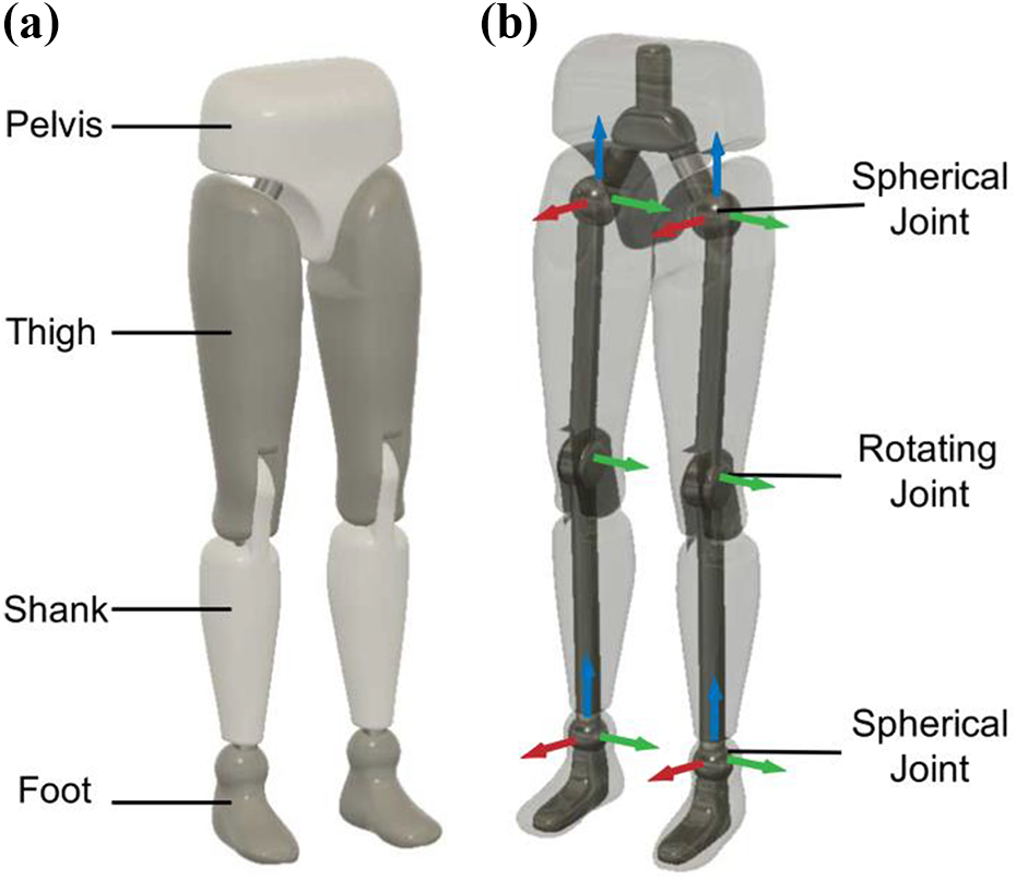
The core structure of the lower limb of the human body is a skeleton composed of nearly rigid bones. Each leg is composed of a thigh, a calf, and a foot in series. At the same time, the lower limb combines left and right legs in parallel. The joint is the hub of mutual movement between the bones. The hip joint connects the pelvis and the thigh. The knee joint connects the thigh and the shank. And the joint between the calf and the foot is ankle joint, as shown in Figure 1(b).

The joints of a lower limb can be modeled as a spherical joint within the considered range of movement.³⁶ Referring to the fundamental and basic axes defined in the anatomy, the basic forms of joint motion can be classified into three categories: flexion/extension (FE) around the frontal axis, abduction/adduction (AA) around the sagittal axis, and internal/external (IE) around the vertical axis. Degrees of freedom (DOF) is used as a term to describe the freedom of motion. Since the muscles around each joint are different from the ligament constraints, the freedom of movement of each joint is also different, as shown in Figure 1(c). The hip joint has 3-DOF, which are hip flexion/extension (HFE), hip abduction/adduction (HAA), and hip internal/external (HIE). One degree of freedom at the knee joint, that is, knee abduction/adduction (KFE), and 3-DOF at ankle joint, which are ankle flexion/extension (AFE), the ankle abduction/adduction (AAA), and the ankle internal/external (AIE). The rotation of each joint degree of freedom is limited by the structure of the lower limb of the human body, and they have the upper and lower limited angle of rotation, we set the initial angle at each joint DOFs in the standing state to 0, so the range of motion angle at each joint’s DOFs can be consulted in Table 1.

Table 1.

Movement form and the motion angle range for hip, knee, ankle joints.

Joint	DOF(s)	Movement form	Angle range (min) to (max)
Hip	3	Hip internal/external (HIE)	(−120°) to (65°)
		Hip abduction/adduction (HAA)	(−30° to −35°) to (40°)
		Hip extension/flexion (HEF)	(−15° to −30°) to (60°)
Knee	1	Knee extension/flexion (KEF)	(−120° to −160°) to (0°)
Ankle	3	Ankle internal/external (AIE)	(−15°) to (30° to −50°)
		Ankle abduction/adduction (AAA)	(−20°) to (40° to 50°)
		Ankle extension/flexion (AEF)	(−30° to −35°) to (15° to 20°)

DOF: degrees of freedom.

Walking is the most common form of movement for humans. Since the walking process is periodically changed, the description of the walking state is usually expressed by a gait cycle when studying the mechanism of human gait, and the whole walking process is a plurality of approximations with continuous convergence of the same gait cycle. According to the contact relationship between the human foot and the ground, there are two different states of single foot support and double foot support. For one leg, the movement can be divided into a standing phase and a swing phase during a gait cycle. The walking state of the human body can be regarded as the process of alternate support phase and swing phase of the legs with a half gait cycle delay between left and right legs. In Figure 2, the gait diagram describes the movement of the right during one gait cycle. Keyframe with red color indicates that the leg is at supporting state while green color indicates the leg is at swing state.

Figure 2.

A whole gait cycle of the single leg (right leg) during the walking process.

LLE structure configuration

The exoskeleton robot is a kind of wearable human–machine device. In order to provide more anthropomorphic motion, the LLE robots need to be designed according to the physiological structure of the human body. In theory, the lower extremity exoskeleton robot should provide the lower limb DOFs as described in Figure 1(c), to provide complete walking assistance. However, for the purpose of straight walking, the internal/external DOF of the hip joint (HIE) and ankle joint (AIE) can be ignored because they contribute to the turning movement along the vertical axis. The LLE robot’s degrees of freedom configuration are shown in the Figure 3(a). The DOFs configuration of the LLE’s right leg is as follows: 2-DOF of HAA and HEF at the hip joint, 1-DOF of KEF at the knee joint, and 2-DOF of AAA and AEF at the ankle joint. In the LLE’s left leg side has the same DOFs configuration as the right leg. In actual scene, each degree of freedom corresponds to an actuator. Figure 3(b) shows the proposed LLE structure whose actuated joints aligned with the joints of the human body.

Figure 3.

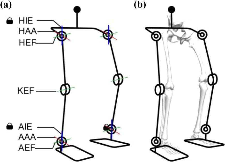
(a) 5-DOF configuration of LLE’s single leg (right leg). DOFs with a lock icon beside means it is unused or inactivated. (b) LLE with human skeleton aligning at joints. DOF: degrees of freedom; lower limb exoskeleton.

Human–exoskeleton coupling system modeling

The LEE coupling system with the LLE and the human body can be regarded as limb chain model which made up from one exoskeleton chain and one human body chain. These two kinematic chains are coupled as the human body chain by adding rigid or flexible constraints to some parts of the exoskeleton chain. During the movement of the coupling system, the exoskeleton chain transmits the force and moment to the human body chain through the connector to complete the movement. In this section, we propose the human–exoskeleton coupling system and its dynamic simulation modeling using Fusion360 and MATLAB/Simulink Multibody.

The human–machine coupling system is a complex nonlinear dynamic system. It takes a lot of effort to deal with the kinematic and dynamic equations. We build a dynamic simulation environment using MATLAB/Simulink Multibody. With the help of physics-based modeling method, we can get rid of the complex kinematic and dynamic modeling. Based on the analyze of human lower limb and the LLE structure configuration in the “Human physiology and LLE structure” section. We establish a virtual coupling system with three main parts:

human lower limb chain;

LLE robot chain; and

coupling two chains and interact with the environment.

Human lower limb chain

The human lower limb chain is the passive kinematic chain in the human–machine coupling system. We design the human lower limb chain model using Autodesk Fusion360.³⁷ It is hard to realize the complex physiological structure of the human body. To simplify the difficulty of modeling, the human lower limb chain in this article is designed by a hierarchy of rigid bodies, which have one pelvis link, two thigh links, two shank links, two feet links, and several joints connect the adjacent links, shown in Figure 4(a). The joints between pelvis link and thigh link in both legs are 3-DOF hip joints, we use a spherical joint which can rotate along three orthogonal axes. The joint between thigh and shank in both legs is the knee joints, we use a 1-DOF revolute joint in the modeling. The joint between shanks and feet are the ankle joints, we also use 3-DOF spherical joints to represent the ankle joints, as illustrated in Figure 4(b). The human lower limb parameter is measured from a 180 cm tall, 75 kg weighted male, and the model-related parameters are shown in Table 2.

Figure 4.

Human lower limb chain modeling. (a) The hierarchy of rigid bodies represents for the human skeleton. (b) Joints with the specified axes as the reference revolution axes of each DOF. DOF: degrees of freedom.

Table 2.

Model-related parameters.

Part	Parameter
Torso	350 mm (width)
Thigh	420 mm (length)
Shank	405 mm (length)
Foot	210 mm (length)

The human lower limb kinematic chain modeling process in MATLAB/Simulink Multibody is illustrated in Figure 5. The schemes whose two main branches create two legs of the human lower limb body chain with their upper endpoint connect to the pelvis part.

Figure 5.

Human chain modeling scheme in MATLAB/Simulink Multibody.

LLE robot chain

According to the LLE structure proposed in the “Human physiology and LLE structure” section, we designed the LLE chain using Autodesk Fusion360. The main structure configuration is as follows: each leg has four-link modules and five drive joints equipped with actuators. Four-link modules are hip module, thigh module, shank module, and foot module, respectively. As shown in Figure 6, the figure only shows the actuator distribution of the right leg, and the left leg is symmetrical with the right leg. So, there are 10 actuators in total in LLE robot chain of the coupling system. What’s more, the thigh frame segment and the shank frame segment are adjustable in length to align the joints of exoskeleton chain with the joints of human body chain. The LLE chain simulation modeling process in MATLAB/Simulink Multibody is illustrated in Figure 7.

Figure 6.

LLE chain modeling. LLE: lower limb exoskeleton. (a) Perspective view, (b) Side view.

Figure 7.

A single leg of LLE chain modeling scheme in MATLAB/Simulink Multibody. LLE: lower limb exoskeleton.

System integration

Coupling limb chain model: During the movement of the coupling system, the exoskeleton chain transmits the force and moment to the human body chain through the connector to complete the movement. In our research, two kinematic chains are coupled with rigidity constraints in three parts, as shown in Figure 8(a).

Pelvis of human lower limb chain and trunk of LLE chain.

Left foot of human lower limb chain and left foot link of LLE chain.

Right foot of human lower limb chain and right foot link of LLE chain.

While other parts of both the human body chain and LLE chain are set free without any constrains. The modeling process in MATLAB/Simulink is shown in Figure 8(b), we use three transform blocks to set the position of connected parts suitable for combining.

Interact with environment: When the coupling system walking on the ground, the LLE chain holding the human lower limb chain at a rigidly connected part, and interacts with ground at plantar at the same time. The coupling system move as desired motion depending on the plantar contact with the ground. So, we need to build the contact law between LLE chain’s plantar and ground. In our study, we employ a group of Sphere to Plane Force from Multibody Contact Force Library, and fix the sphere component at the four corners of foot link bottom side, as illustrated in Figure 9. The contact force parameters are set as follows: contact stiffness is 2500 N/m, contact damping is 100 N/(m/s), coefficient of kinetic friction and static friction are 0.7 and 0.8, respectively.

Motion transmission: The motion transmission procedure of the coupling system can be depicted as shown in Figure 10, with the following process. First, the LLE joint trajectory is produced by a system control unit. Then, the LLE chain is driven by the reference joint trajectory. Next, the movement of the LLE chain drives the human body chain due to the rigid connect at the coupling position. Finally, we can get the joint trajectory of human limb chain, which has a great significance in the further analysis of the coupled system.

Figure 8.

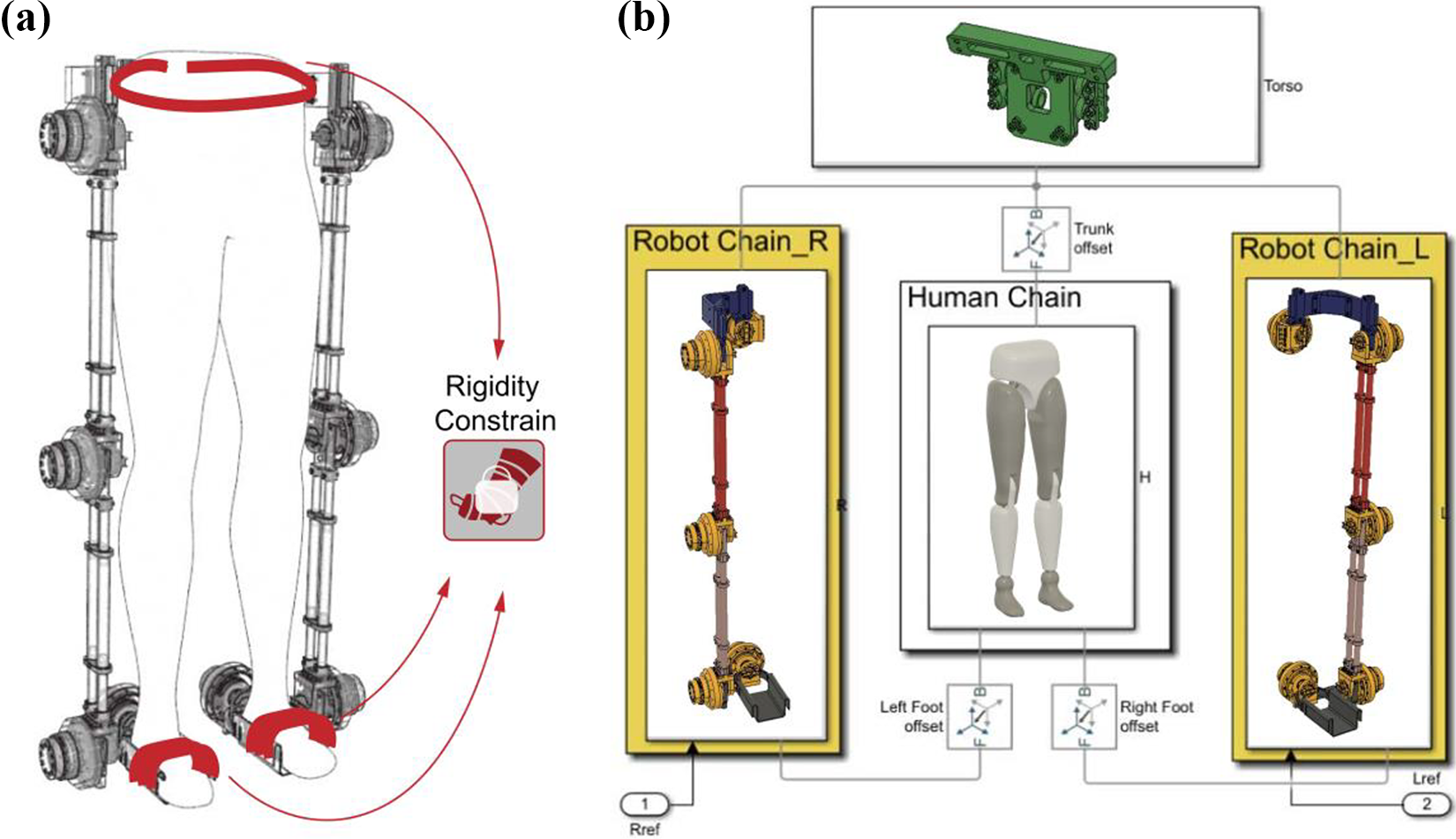
Coupling solution of a two-chain system. (a) Rigidly combined at the pelvis and two feet. (b) The modeling process in MATLAB/Simulink Multibody.

Figure 9.

Contact force configurated at both plantar of LLE chain’s foot links. LLE: lower limb exoskeleton.

Figure 10.

Motion transmission procedure of coupling system.

Gait trajectory optimization based on GA

In this section, we focus on the gait trajectory generation for the human–exoskeleton coupling system. With the help of a virtual multibody simulation environment, we can directly use forward dynamic simulation to analyze the coupling system by sensing the virtual system’s relative signal. To generate a more natural gait trajectory for the coupled system according to the walking mechanism, we employ a GA method to generate the gait trajectory.

GAs are heuristic search approaches that are applicable to a wide range of optimization problems. This method based on Darwin’s Natural Evolution Theory. They work with a population of initial solutions, called chromosomes, which are evolved through several operations during a certain number of generations, usually reaching a well-optimized solution, and preserving the best individuals according to a specific evaluation criterion. In order to accomplish this, in each generation, the chromosomes are individually evaluated using a function that measures its performance, called fitness function. The chromosomes with the best fitness values are selected to generate the next generation applying the crossover and mutation operations. Thus, each new generation tends to adapt and improve the quality of solutions, until we obtain a solution that satisfies a specific objective. The GA implementation used in our coupled system is based on the Optimization toolbox-GA in MATLAB.

In the coupled system, we use a basic GA described by Oliver Kramer.³⁸ Algorithm 1 shows a summary of the GA used to evolve the coupled system’s gait parameters in Table 3.

Table 3.

A basic GA described by Oliver Kramer.

Algorithm 1 The pseudocode of the GA

GA: genetic algorithm.

Individual-gait trajectory

As we discussed before, the coupled system transmits the movement of the activated exoskeleton chain to the passive human body chain. And the movement of the exoskeleton was inspired by the joint trajectory at each actuator-equipped joint which comes from the system control unit. So, the trajectory of joints is treated as the chromosome in a GA which is subject to the optimization process.

The protagonist in a GA is a mutation. Mutation operators change a solution by disturbing them. A mutation is based on random changes. There are there main requirements for mutation operator: reachability, unbiasedness, and scalability. Reachability means each point in solution space must be reachable from an arbitrary point in solution space. Unbiasedness indicates mutation operator should not induce a drift of the search in a particular direction, at least in unconstrained solution spaces without plateaus. Scalability means each mutation operator should offer the degrees of freedom that its strength is adaptable. In the GA we designed, the solution space (joint trajectory) is completely covered by continuous vectors with limited range (joint angle range). The random resetting mutation operator is chosen which randomly chooses a replacement for each selected individual. The mutation rate is practically fixed in order to not induce a drift of the search in a particular direction.

Finite-state machine

In our study, the finite-state machine (FSM) method is used as the fundamental principle in generating the joint trajectory. A FSM is an abstract machine that can be in exactly one of a finite number of states at any given time. We can simply divide the (K)th walking period into N pieces subperiod by N + 1 state, where the last state indicates the junction locating at the end of the (K)th walking period and the beginning of the (K + 1)th walking period, as illustrated in Table 4.

Table 4.

Finite-state machine table.

Joint	S ₁	S ₂	…	S_N	$S_{N + 1}$
HAA	$θ_{1}^{H A A}$	$θ_{2}^{H A A}$	…	$θ_{N}^{H A A}$	$θ_{1}^{H A A}$
HEF	$θ_{1}^{H E F}$	$θ_{2}^{H E F}$	…	$θ_{N}^{H E F}$	$θ_{1}^{H E F}$
KEF	$θ_{1}^{K E F}$	$θ_{2}^{K E F}$	…	$θ_{N}^{K E F}$	$θ_{1}^{K E F}$
AAA	$θ_{1}^{A A A}$	$θ_{2}^{A A A}$	…	$θ_{N}^{A A A}$	$θ_{1}^{A A A}$
AEF	$θ_{1}^{A E F}$	$θ_{2}^{A E F}$	…	$θ_{N}^{A E F}$	$θ_{1}^{A E F}$

HAA: hip abduction/adduction; HEF: hip internal/external; KEF: knee abduction/adduction; AAA: ankle abduction/adduction; AEF: ankle internal/external.

Formulating trajectory

Although the walking trajectory has been properly designed by using the FSM, we still need to formulate the trajectory to become a time-continuous smooth trajectory as the input of a coupled system. The continuity, stability, and smoothness of the cubic spline interpolation method have been applied in the gait planning of the lower limb carrying exoskeleton.¹⁶ Since we have several waypoints needed to approximate, we can get a piecewise time-continuous trajectory whose every single piece function between two waypoints can be described by a third-order function as the following expression

{}^{S}θ (t) = a_{0} + a_{1} \times t + a_{2} \times t^{2} + a_{3} \times t^{3}, (t \in (S_{i}, S_{i + 1}))

where t represents any time between two adjacent states in the state machine (e.g. S). In fact, we employ the spline interpolation method in MATLAB to formulate the trajectory as the user guide. The reference trajectories of joint variables are formulated by Spline function, which can consult from the introduction in MATLAB documentation

θ = S p l i n e (T_{i}, θ_{i}, t), (i = 1, ..., S + 1)

Function Spline indicates that we can get the formulated result joint angle θ at any given time t in a gait period, T_i denotes the moments in gait period of waypoints, θ_i denotes the angle variants of corresponding waypoints.

Because the movement of the lower limbs of the human body is periodically changed in the form of alternating swings of the legs. Two legs can simply be considered as that they share the same gait trajectory while there is a half gait period delay between two legs. By this way, the input of a coupled system which can also be treated as the Genome in the GA is

P a r a = S \times J

where S denotes the state numbers, which we define in the FSM table (Table 2). J denotes the drive joint numbers of a single leg in the exoskeleton chain. In this study, S = 6, J = 5.

Fitness function

An important part of the GA is the fitness function. We designed a set of gradually improved fitness function as the objective of the optimization gait trajectory generated by GA. In the iterative process of GA, the fitness function F used to evaluate the performance of the generated gait trajectory for the coupled system is shown as equation (4). The coupled system will execute the gait trajectory in the simulation environment and perform a walking movement. We use some of the data in walking performance as the influential factors in the fitness function. More specifically, we define survive time T, covered distance D, torso’s angular velocity $ω_{a v g}$ , joint trajectory aggressiveness $A g g$ , and plantar contact force f_P as an influential factor. All of the coordinate-related parameters are defined in a world-aligned coordinate frame. Each right-hand term in equation (4) is acquired by integrating a time-dependent measure during simulation

F = F i t n e s s F u n c t i o n (D, T, ω_{a v g}, f_{P}, A g g)

In the early-stage experiments, we use survive time T and covered distance D as the influential factors in the fitness function

F = D \times T

Survive time T

Survive time T denotes the terminate time about the simulation of every individual. During the simulation, we terminate a simulation prematurely when failure or fatal error is detected to save on simulation time and to help prevent local minima in the optimization. There are several parameters that we used to terminate the simulation. Firstly, we judge the failure by the height of center-of-trunk, which means if the trunk coordinate along Z-axis is below 0, the simulation of this individual stop immediately because it indicates this individual has fallen. Secondly, we terminate the simulation when the distance in lateral direction is too far away from the original walking following line. So, either of these two parameters is approaching the limited value, it is unnecessary to go on the following simulation. By the way, the simulation time is 10 times longer than the normal gait cycle. In other words, if a gait trajectory individual is stable enough, it can go through the full simulation time

T = t_{e n d}

Covered distance D

The covered distance D is computed by the geometric position of trunk vary along the X-axis at the end of simulation. We encourage those individuals who can walk through a complete simulation time and arrive at a farther destination. We consider this influential factor can do great help in searching feasible solutions in the solution space

D = X (t_{e n d})

However, the results of the early-stage experiment are not very satisfactory by using survive time and covered distance as the influential factors to guide the direction of evolution. In fact, the selected individuals are the ones with exaggerated gait. It seems like a crown walking on tiptoes, large strides, and the torso is always in a backward trend. By intuitively observing large stride gait and common gait from normal people, we summarize that a gentler gait will produce a slight contact force at plantar for the purpose of protecting the physiological joints and saving metabolic energy. To dodge the previous embarrassing result, we add the plantar contact force f_P which intimate the adverse consequences of large stride and walking on tiptoes as another important influential factors. Thus, the fitness function in the middle-stage experiments is improved through the equation

F = (D \times T) / f_{P}

Plantar contact force f_N

During the simulation, the plantar contact force is the key element to enable the interaction between the coupled system and world ground. In our study, each foot has four contact points as setting. $f_{P}^{R_{i}} and f_{P}^{L_{i}}$ represent the contact force at the corner of plantar. Plantar contact force f_P is simply denoted through the equation

f_{P} = max (\sum_{i = 1}^{4} f_{P}^{R_{i}}, \sum_{i = 1}^{4} f_{P}^{L_{i}})

The gait learning becomes much more efficient by using equation (8). The individuals selected perform a less exaggerated gait with smaller stride. But we found a lot of solutions are still weird through visualizing the obtained solution. These individuals showed unstable gaits like drunkenness or jittering legs. Thus, besides the contact force at the plantar, the stability of torso and the aggressiveness of legs play an important role in obtaining a natural gait. We add two more influential factors, average angular velocity $ω_{a v g}$ and trajectory aggressiveness $A g g$ , to fitness function through the equation

F = (D \times T) / (f_{P} \times ω_{a v g} \times A g g)

Average angular velocity $ω_{a v g}$

For average angular velocity $ω_{a v g}$ , it is made up of $ω_{a v g}^{x}$ _, $ω_{a v g}^{y}$ , and $ω_{a v g}^{z}$ _. These three parameters represent the torso’s orientation along the x-axis, y-axis and z-axis of the world coordinate system respectively. The amplitude of any one of these factors will increase the extent of average angular velocity $ω_{a v g}$ . Large average angular velocity indicates that the torso’s shaking is intense during the walking movement. However, a stable walking posture requires a minor change of torso’s shaking. The average angular velocity of torso is expected to get more moderate during the optimization. The quantified expression is shown as follows

ω_{a v g} = ω_{a v g}^{x} + ω_{a v g}^{y} + ω_{a v g}^{z}

Trajectory aggressiveness $A g g$

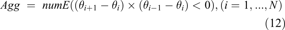
For the trajectory aggressiveness Agg, it describes the oscillation of one gait trajectory cycle. If one gait trajectory with a lot of bouncing up and down or a lot of inflection points, we consider this gait trajectory is worse. We use the following evaluating method to guide the optimization of gait trajectory to a gentler direction. Function numE in equation (8) means the number of elements that satisfy the condition in the parentheses. If the sign of the adjacent two elements is different in the differential sequence of the gait trajectory, it indicates the gait trajectory has fluctuated within this interval. Every fluctuation will increase the trajectory of aggressiveness Agg. When we are searching for a natural gait trajectory, individuals with large trajectory aggressiveness will be eliminated when finding the optimal solution

A g g = n u m E ((θ_{i + 1} - θ_{i}) \times (θ_{i - 1} - θ_{i}) < 0), (i = 1, ..., N)

The above factors which evaluate the performance of gait trajectory have different desire tendency during the optimization. We expect some factors the larger the better while some factors the smaller the better. Overall, the above four factors can be classified into two categories: reward factors and penalty factors. The covered distance D and the survive time T are considered as reward factors, while the plantar contact force f_P , the average angular velocity $ω_{a v g}$ , and the trajectory aggressiveness $A g g$ is considered as penalty factors.

Experiment and result

In this section, we exhibit the accomplished experiments using MATLAB/Multibody modeling environment and Optimization toolbox-GA in MATLAB, version r2019a, using the ode15s solver with the auto variable step. Our intention is to generate a more natural gait trajectory for our proposed coupled system using a GA. The parameters of GA are initialized and executed as shown in Table 5. The last parameters value Random (50) for initial population means the gait trajectory (individual) is randomly obtained according to the limitation angle of joints (Table 5).

Table 5.

GA parameters.

Parameters	Value
Population size	50
Number of generations	50
Crossover	0.8
Mutation	0.05
Fitness Function	(10)
Gait period(s)	0.8
Number of states	6
Initial population	Random (50)

GA: genetic algorithm.

We set the gait period 0.8 s, and the simulation time is 10 s. The simulation environment gravity acceleration g = 9.80665 m/s². The coupled system works as follow in every single simulation:

The coupled system is placed in the starting position and orientation in the simulation environment.

Loading the FSM-based gait trajectory generated by GA.

Executing the physical simulation and sensing data for optimization.

Calculating the performance of gait trajectory.

We carry out three experiments in order to explore the performance after adding different impact factors to fitness function (equations (5), (8), and (10)). The experiment arrangement is described in Table 6.

Table 6.

Experiment arrangement.

Experiment	Fitness function	Equation
01	$F = D \times T$	(5)
02	$F = (D \times T) / f_{P}$	(8)
03	$F = (D \times T) / (f_{P} \times ω_{a v g} \times A g g)$	(10)

Results of experiment 01

Through the iteration of a GA, we obtain the optimized individual at the end of the iteration. Figure 11 shows the generated gait animation screenshot of experiment 01 which using equation (5) as the fitness function in the GA. From the movement frame illustrated in Figure 11, the result of this experiment is not satisfactory through intuitive observation. The walking action is a little bit exaggerated. It seems like hitting the ground with pedal heavily, large stride, and the torso is always in a backward trend. Comparing the gentle gait with this exaggerated gait, we conjecture that the pedal contact force is the main difference between them. So, we gather the contact force at the pedal, as the graph shown in Figure 12. In Figure 12, there is a large contact force generated when pedal contact with ground. The maximum value up to 225 N.

Figure 11.

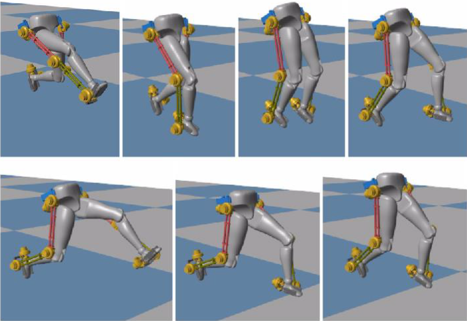
Movement animation screenshot of experiment 01.

Figure 12.

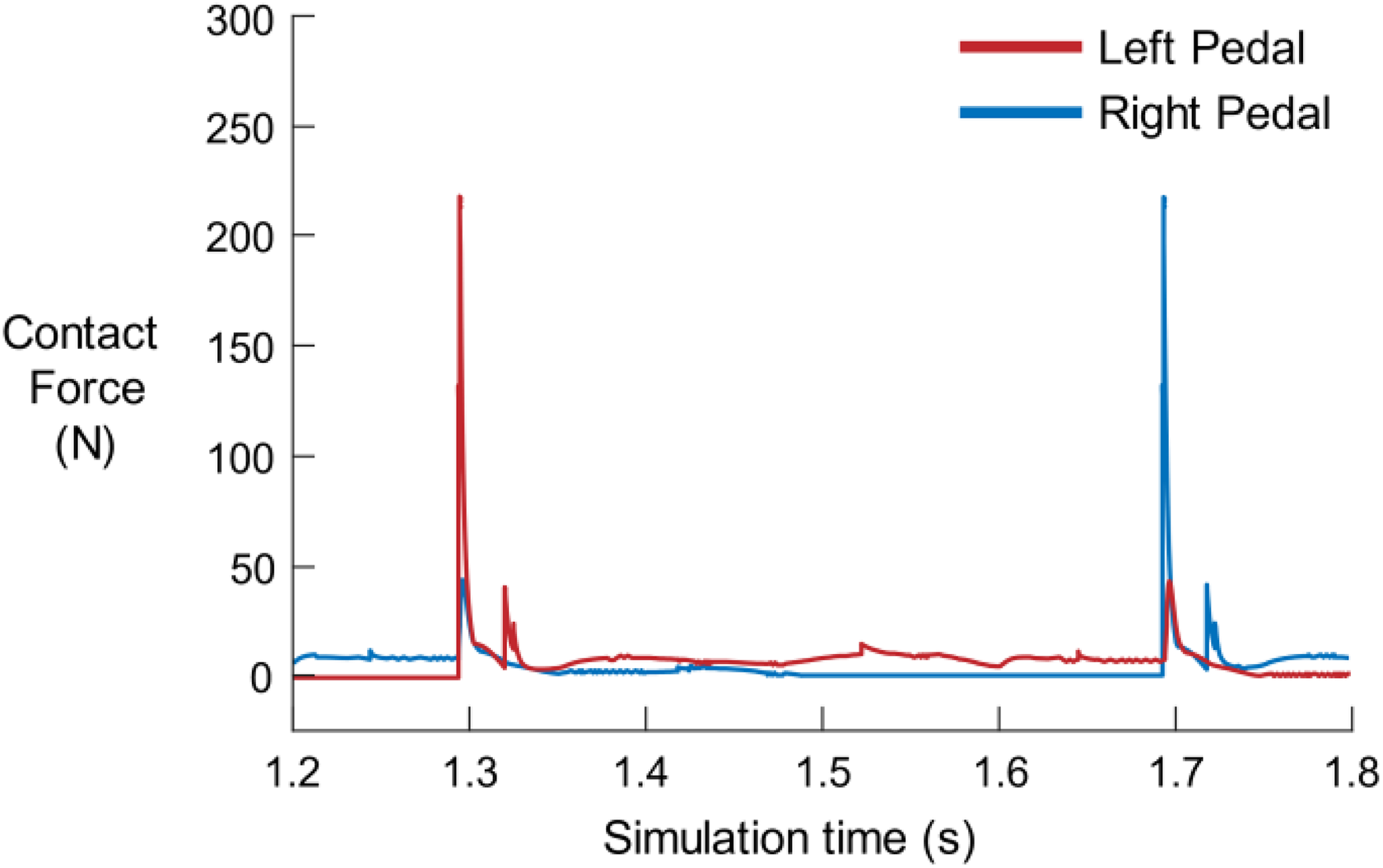
The pedal contact force of experiment 01.

Results of experiment 02

In this experiment, the pedal contact force is taken into account. Figure 13 shows the generated gait animation screenshot of experiment 02 which using equation (8) as the fitness function in the GA. From the movement frame illustrated in Figure 13, we can observe the walking action become much more moderate. The stride is no longer as large as in the previous experiment. We collect the pedal contact force as shown in Figure 14. The maximum value of pedal contact force on both sides are under 55 N. However, the tendency of backward overturn is still not improved. This time, we conjecture that the torso stability is the main issue. So, we gather the angular velocity at torso, as the graph shown in Figure 15. In Figure 15, the angular velocity along sagittal axis (x), frontal axis (y), vertical axis (z) changing within the range from −0.05 rad/s to 0.08 rad/s.

Figure 13.

Movement animation screenshot of experiment 02.

Figure 14.

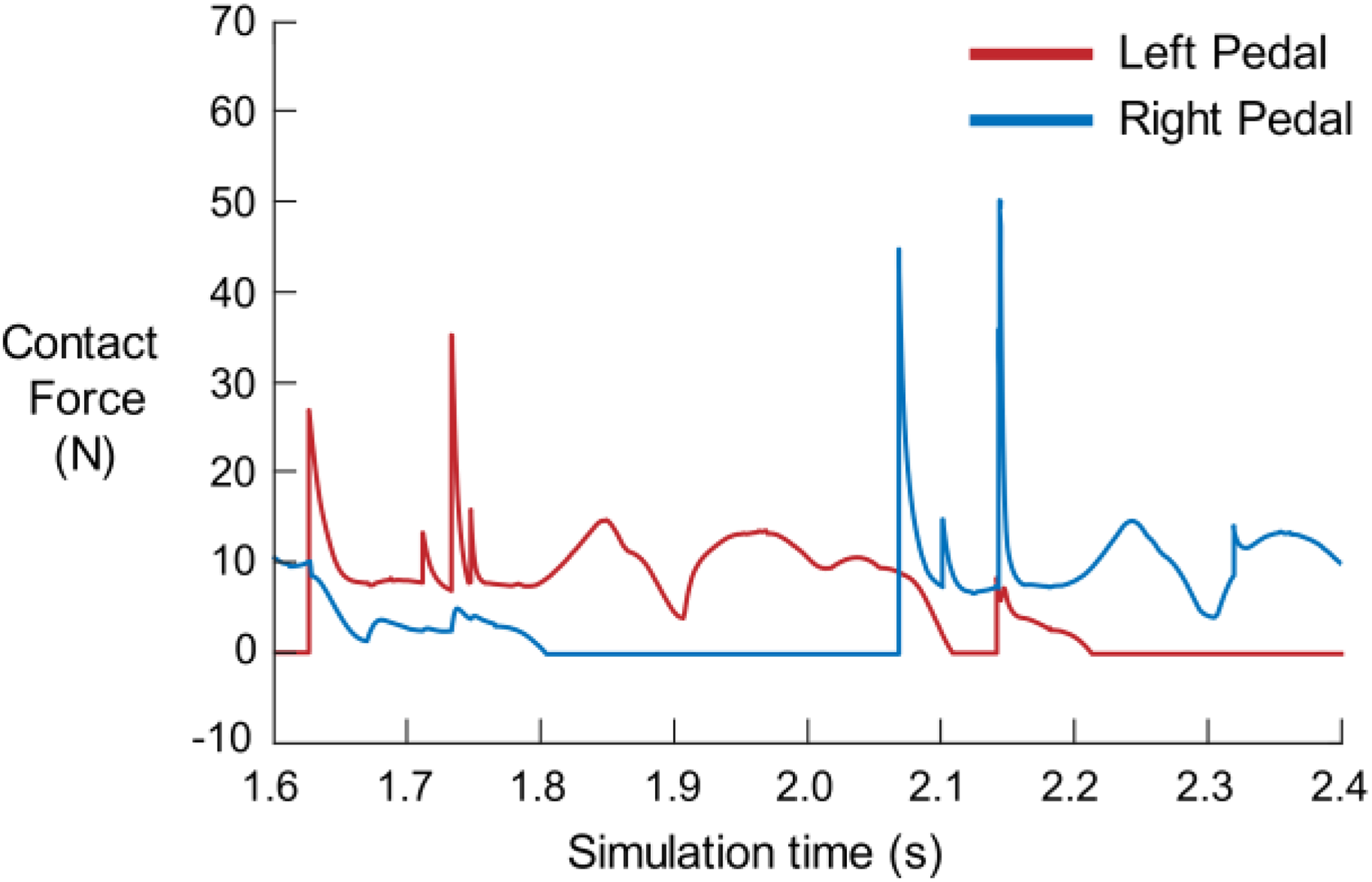
The pedal contact force of experiment 02.

Figure 15.

Torso angular velocity of experiment 02.

Results of experiment 03

We carry out this experiment with the aim of reducing torso instability. In this experiment, besides the fitness function from equation (10), the remaining parameters are the same as the previous two experiments. Figure 16 shows the generated gait animation screenshot of experiment 03. From the movement frame illustrated in Figure 16, we can intuitively find that the walking action in experiment 03 is as moderate as the walking action in experiment 02. We gather the pedal contact force and torso angular velocity as shown in Figures 17 and 18. On one hand, according to the data from Figure 17, we can recognize that the maximum value of the pedal contact force has increased a little bit compared with experiment 02. But it is still less than the pedal contact force in experiment 01. On the other hand, the angular velocity range along sagittal axis (x), frontal axis (y), vertical axis (z) is smaller than experiment 02, which is from −0.03 rad/s to 0.05 rad/s.

Figure 16.

Movement animation screenshot of experiment 03.

Figure 17.

The pedal contact force of experiment 03

Figure 18.

Torso angular velocity of experiment 03.

Discussion

In the beginning, we believe that we can get a gait trajectory close to nature with the original fitness function (equation (5)). But as we can see in Figure 11, the motion of our coupled system seen like a crown walking on tiptoes, and the motion is a little bit strange with large stride, and the torso is always in a backward trend. The reason causing this experiment’s result in our view is mainly due to the lack of constraint parameters. After analyzing the normal walking action, we conjecture the constraint on the pedal contact force may do help in optimization. In fact, the results of experiment 02 prove that adding pedal contact force into fitness function (equation (8)) is a correct decision. In addition, we found that adding angular velocity and trajectory aggressiveness to the fitness function (equation (10)) helps to improve the stability of the generated gait trajectory. However, we have to say, the influential factors cannot completely represent the walking law of stable and smooth gait trajectory. The fitness function will become more and more consummate under further research in the development of this human–machine coupled system.

Through the above experiments and relative results, our proposed human–exoskeleton coupling system is proved that it can provide another way to explore the LLE research field. And the GA-based trajectory generation method is verified that it can generate an optimized gait trajectory in an efficient way if we carefully consider the natural law behind the locomotion.

However, there are also many deficiencies that need to be improved. On one hand, considering that the model has been simplified in this study, we need to add more detail in the coupling system and make it closer to the real working situation. For example, the actuator equipped at each DOF which works with the torque input or current input instead of the angle input used in our simplified model, we have to consider the capability of actuators if we want to implement actual manufacturing. What’s more, the control strategy should also be properly designed for the coupled system which is absent in this work. At the same time, the human limb chain should also use the full-body model to make it closer to real human body. On the other hand, the fitness function utilized in current work could not stand for the nature gait sufficiently, and it is almost impossible to describe the natural gait trajectory completely with mathematical expressions. We need to describe the motion in detail as much as possible by observing and collecting data.

Conclusions

To summarize the major contribution of this study. Firstly, we built a human–machine coupling system for the lower extremity exoskeleton in MATLAB/Simulink Multibody virtual simulation environment. The virtual system is coupled by a power-driven lower extremity exoskeleton chain and a passively moving human lower limb chain. The double-chain coupling system transmits motion through solid-connect constraints at the torso position and the plantar position. Next, we planned the trajectory of the human–body coupling system for the lower extremity exoskeleton. The planning of the motion trajectory is mainly based on the GA, which is iteratively generated under the optimization of a set of specially designed fitness function. Finally, we accomplished a group of experiments to validate the specific fitness function, and it approves that the GA with specially designed fitness function can generate a gait trajectory closer to the natural motion gait. The effort accomplished in this article will establish the foundation for future research and practical applications.

Footnotes

Declaration of conflicting interests

The author(s) declared no potential conflicts of interest with respect to the research, authorship, and/or publication of this article.

Funding

The author(s) disclosed receipt of the following financial support for the research, authorship, and/or publication of this article: This research was funded by the National Natural Science Foundation of China (NSFC grant no. 51775325) and Young Eastern Scholars Program of Shanghai (grant no. QD2016033).

ORCID iD

Bin Ren

Jianwei Liu

References

Makinson

Research and development prototype for machine augmentation of human strength and endurance. Hardiman I project. General Electric Co Schenectady NY Specialty Materials Handling Products Operation, 1971.

Chen

Qin

, et al. Recent developments and challenges of lower extremity exoskeletons. J Orthop Transl 2016; 5: 26–37.

Huo

Mohammed

Moreno

, et al. Lower limb wearable robots for assistance and rehabilitation: a state of the art. IEEE Syst J 2016; 10(3): 1068–1081.

Yan

Cempini

Oddo

, et al. Review of assistive strategies in powered lower-limb orthoses and exoskeletons. Robot Auton Syst 2015; 64: 120–136.

Riener

Lunenburger

Jezernik

, et al. Patient-cooperative strategies for robot-aided treadmill training: first experimental results. IEEE Trans Neural Syst Rehabil Eng 2005; 13(3): 380–394.

Wang

Liu

. Underactuated robotics: a review. Int J Adv Robot Syst 2019; 16(4): 1–29.

Zhang

Liu

, et al. Dynamics analysis and numerical simulation of a novel underactuated robot wrist. Proc Inst Mech Eng B 2017; 231(12): 2145–2158.

Banala

Kim

Agrawal

, et al. Robot assisted gait training with active leg exoskeleton (ALEX). IEEE Trans Neural Syst Rehabil Eng 2009; 17(1): 2–8.

Pransky

The Pransky interview: Russ Angold, co-founder and president of Ekso™ Labs. Ind Robot Int J 2014; 41(4): 329–334.

10.

Talaty

Esquenazi

Briceno

(eds) Differentiating ability in users of the ReWalk™ powered exoskeleton: an analysis of walking kinematics. In: 2013 IEEE 13th international conference on rehabilitation robotics (ICORR), 24–26 June 2013. Seattle, WA, USA: IEEE.

11.

Farris

Quintero

Murray

, et al. A preliminary assessment of legged mobility provided by a lower limb exoskeleton for persons with paraplegia. IEEE Trans Neural Syst Rehabil Eng 2013; 22(3): 482–490.

12.

Zoss

Kazerooni

Chu

. Biomechanical design of the Berkeley lower extremity exoskeleton (BLEEX). IEEE-ASME Trans Mech 2006; 11(2): 128–138.

13.

Swift

. Control and trajectory generation of a wearable mobility exoskeleton for spinal cord injury patients. Berkeley: University of California, 2011.

14.

Sankai

. HAL: hybrid assistive limb based on cybernics. In: Kaneko

Nakamura

(eds) Robotics research. Springer tracts in advanced robotics, vol. 66. Berlin, Heidelberg: Springer, 2010, pp. 25–34.

15.

Kim

Lee

Kim

, et al. (eds) Mechanical design of the Hanyang exoskeleton assistive robot (HEXAR). In: 2014 14th international conference on control, automation and systems (ICCAS 2014), 22–25 October 2014. Seoul, South Korea: IEEE.

16.

Wang

Tian

Han

, et al. ZMP theory-based gait planning and model-free trajectory tracking control of lower limb carrying exoskeleton system. Stud Inform Control 2017; 26(2): 161–170.

17.

Panich

. Design and simulation of leg-exoskeleton suit for rehabilitation. Glob J Med Res 2012; 12(3).

18.

Dumitru

Copilusi

Geonea

, et al. Dynamic analysis of an exoskeleton new ankle joint mechanism. In: Flores

Viadero

(eds) New trends in mechanism and machine science, vol. 24. Cham: Springer, 2015, pp. 709–717.

19.

Zhang

Zhu

, et al. Skeleton model-based approach to integrated engineering design and analysis. Int J Adv Manuf Tech 2016; 85(5-8): 1105–1115.

20.

Geijtenbeek

Panne

Stappen

. Flexible muscle-based locomotion for bipedal creatures. ACM Trans Graphic 2013; 32(6): 1–11.

21.

Smith

. inventor. Open Dynamics Engine User Guide v0.5. 2005.

22.

Heinen

Osório

(eds) Applying genetic algorithms to control gait of physically based simulated robots. In: 2006 IEEE international conference on evolutionary computation, 16–21 July 2006. Vancouver, BC, Canada: IEEE.

23.

Heinen

Osorio

(eds) Applying genetic algorithms to control gait of simulated robots. In: Electronics, robotics and automotive mechanics conference (CERMA 2007), 25–28 September 2007. Morelos, Mexico: IEEE.

24.

Aliman

Ramli

Haris

(eds) Modeling and co-simulation of actuator control for lower limb exoskeleton. In: 2018 3rd international conference on control and robotics engineering (ICCRE), 20–23 April 2018. Nagoya, Japan: IEEE.

25.

MSCT. MATLAB and Simulink Robotics Arena: Walking Robot GitHub: MathWorks Student Competitions Team, https://www.github.com/mathworks/msra-walking-robot (2019, accessed 23 April 2019).

26.

Miskon

MFB

Yusof

MBAJ

(eds). Review of trajectory generation of exoskeleton robots. In: 2014 IEEE international symposium on robotics and manufacturing automation (ROMA), 15–16 December 2014. Kuala Lumpur, Malaysia: IEEE.

27.

Dip

Prahlad

Kien

. Genetic algorithm-based optimal bipedal walking gait synthesis considering tradeoff between stability margin and speed. Robotica 2009; 27(3): 355–365.

28.

Wang

Qian

Zhang

, et al. Gait trajectory planning and simulation for the powered gait orthosis. In: 2007 IEEE international conference on robotics and biomimetics (ROBIO), 15–18 December 2007. Sanya, China: IEEE.

29.

Biagiotti

Melchiorri

. Trajectory planning for automatic machines and robots. Berlin Heidelberg: Springer-Verlag, 2008.

30.

Gomes

Siqueira

AAG

Gobbo

(eds) Improving the parameters of neural oscillators to generate joint trajectories of an exoskeleton for lower limbs. In: 2011 9th IEEE international conference on control and automation (ICCA), 19–21 December 2011. Santiago, Chile: IEEE.

31.

Bae

Tomizuka

. A gait rehabilitation strategy inspired by an iterative learning algorithm. Mechatronics 2012; 22(2): 213–221.

32.

Shao

Xiang

Liu

, et al. Conceptual design and dimensional synthesis of cam-linkage mechanisms for gait rehabilitation. Mech Mach Theory 2016; 104: 31–42.

33.

TeachMeAnatomy. The lower limb, https://teachmeanatomy.info/lower-limb/ (2019, accessed 12 December 2018).

34.

Yuan

Chen

, et al. Mechanical design and human-machine coupling dynamic analysis of a lower extremity exoskeleton. In: Huang

Liu

Yin

(eds) Intelligent robotics and applications. Lecture notes in computer science, vol. 10462. Cham: Springer, 2017, pp. 593–604.

35.

Delp

Anderson

Arnold

, et al. OpenSim: open-source software to create and analyze dynamic simulations of movement. IEEE Trans Biomed Eng 2007; 54(11): 1940–1950.

36.

Cereatti

Margheritini

Donati

, et al.

Is the human acetabulofemoral joint spherical?

J Bone Joint Surg Br Vol 2010; 92(2): 311–314.

37.

Autodesk. Fusion-360 Overview, https://www.autodesk.com.cn/products/fusion-360/overview (2019, accessed 1 May 2018).

38.

Oliver

. Genetic algorithm essentials. Cham: Springer, 2017.

Simulating human–machine coupled model for gait trajectory optimization of the lower limb exoskeleton system based on genetic algorithm

Abstract

Keywords

Introduction

Materials and methods

Human physiology and LLE structure

Anatomy of human body

LLE structure configuration

Human–exoskeleton coupling system modeling

Human lower limb chain

LLE robot chain

System integration

Gait trajectory optimization based on GA

Individual-gait trajectory

Finite-state machine

Formulating trajectory

Fitness function

Survive time T

Covered distance D

Plantar contact force fN

Average angular velocity ω a v g

Trajectory aggressiveness A g g

Experiment and result

Results of experiment 01

Results of experiment 02

Results of experiment 03

Discussion

Conclusions

Footnotes

Declaration of conflicting interests

Funding

ORCID iD

References

Plantar contact force f_N

Average angular velocity $ω_{a v g}$

Trajectory aggressiveness $A g g$