Inverse kinematic solution of 6R robot manipulators based on screw theory and the Paden–Kahan subproblem

Abstract

The traditional Denavit–Hatenberg method is a relatively mature method for modeling the kinematics of robots. However, it has an obvious drawback, in that the parameters of the Denavit–Hatenberg model are discontinuous, resulting in singularity when the adjacent joint axes are parallel or close to parallel. As a result, this model is not suitable for kinematic calibration. In this article, to avoid the problem of singularity, the product of exponentials method based on screw theory is employed for kinematics modeling. In addition, the inverse kinematics of the 6R robot manipulator is solved by adopting analytical, geometric, and algebraic methods combined with the Paden–Kahan subproblem as well as matrix theory. Moreover, the kinematic parameters of the Denavit–Hatenberg and the product of exponentials-based models are analyzed, and the singularity of the two models is illustrated. Finally, eight solutions of inverse kinematics are obtained, and the correctness and high level of accuracy of the algorithm proposed in this article are verified. This algorithm provides a reference for the inverse kinematics of robots with three adjacent parallel joints.

Introduction

Robot kinematics includes forward and inverse kinematics, which are considered the basis of trajectory planning and motion control. Forward kinematics is about obtaining the pose of the end effector of robots by choosing a group of joint angles within the workspace, which correspond to a unique solution. According to the known pose of the end effector, the solving of all possible joint angles is regarded as inverse kinematics, for which there are multiple solutions. Due to the widespread use of industrial robots, a number of researchers have become interested in exploring the inverse kinematics of 6-degree of freedom (DOF) robot manipulators. In terms of engineering applications, the inverse kinematics of robots is more practical than the forward kinematics. At present, the Denavit–Hatenberg (D-H) parameter ¹ and the screw methods ² are mainly used for kinematics modeling. Although the D-H parameter method is quite popular, it has some disadvantages. The main deficiency is that the kinematic parameters of the D-H model employed for calibration are discontinuous, leading to singularity when the adjacent joint axes of robots are parallel or close to parallel. ^{3 –8} As a result, the actual parameters of this model are difficult to identify, and it cannot be considered as a suitable model for kinematic calibration. ⁹ With the aim of addressing the problem of singularity, several other kinematic models have been proposed, such as the S-model, ¹⁰ the complete and parametrically continuous (CPC) model, ^{11 –13} and the zero reference position model. ¹⁴ Similarly, some other methods ^{15 –19} have also been proposed to avoid the singularities of different robotic systems.

The kinematic calibration of robots involves modeling, measuring, identifying, and compensating. ²⁰ The purpose is to identify the actual kinematic parameters so as to improve the accuracy of robots, while redundant parameters are added to the models mentioned above. ⁹ For calibration, a perfect kinematic model is needed and it should possess completeness, continuity, and no redundancy, while the models listed above do not possess. Fortunately, the product of exponentials (POE) based on screw theory has been adopted as a new kinematics modeling method that can avoid the problem of singularity arising from the kinematic parameters. ^3,8,9,21

Significantly, the POE-based model ⁹ does have the characteristics of completeness, continuity, and no redundancy and is considered the ideal model. Hence, this model is very suitable for kinematic calibration to handle the problem of the execution errors of robots. Currently, many scholars are dedicated to solving the inverse kinematics of robots, focusing on those in which the axes of the last three consecutive joints intersect at a point, while relatively little attention is being paid to researching robots with three adjacent parallel joint axes. The inverse kinematics of the POE method is usually solved according to the known Paden–Kahan subproblem, ² but those subproblems are only applied to cope with the inverse kinematics of the robots with low-DOF.

The most popular modeling method for solving the inverse kinematics of robot manipulators is the D-H method, while the POE method based on screw theory or otherwise is relatively seldom used. The inverse kinematics of the traditional industrial robot, in which the last three joint axes intersect at a point, is solved by combining analytical method with trigonometric equation, and the closed form solutions are obtained. ²² Using the D-H modeling method, a novel numerical iterative method for solving the robot manipulator with 6-DOF is proposed, which is compared with the Newton–Raphson method, and the experimental simulation is given, which proves that the proposed method is superior to the solving method of Newton–Raphson. ²³ Although this iterative algorithm can cope with the inverse kinematics without closed form, it presents poor performance in solving accuracy. The kinematic model of 6R robots is established by employing the method of geometric algebra, and the equations of kinematics are obtained. Then the kinematic problem is transformed into the problem of eigenvalue, and the 16-group solution is determined. ²⁴ Although this method is effective, its error is relatively large. Chen et al. ²⁵ combined the POE simplification method with subproblems to develop an inverse kinematics solver. However, the solver can only solve the inverse kinematics problem of partially nonredundant robots. Aiming at the special structure of the first three joints of 6R robots, Chen et al. ²⁶ adopted the modeling method of screw and proposed a new solving algorithm of subproblem. This algorithm was applied to “Qianjiang Ι” robot, whose last three joint axes intersect at a point, and eight sets of solutions were obtained. Based on the D-H model, Liu et al. ²⁷ utilized the characteristics of special matrices to convert matrix equations of inverse kinematics into corresponding algebraic equations for solution.

In this article, to effectively identify the actual kinematic parameters and correct the execution error of the end effector of robots resulting from deviations in the geometric structure or other factors, the POE method is employed for kinematics modeling. In addition, analytical, geometric, and algebraic methods in combination with the Paden–Kahan subproblem and matrix theory are adopted to solve the inverse kinematic problem of a type of 6-DOF industrial robot, whose three adjacent joint axes are parallel. Real robot products are used, including the universal robots (UR) robot arms of the Universal Robots company and the open unit robot (OUR) robot arms of the AUBO Robotics Technology Company Limited. For the sake of convenience, in the latter part of this article, the OUR-1 robot (as shown in Figure 1) is used as an example. Furthermore, the problems of singularity of the D-H and POE-based models are analyzed from the changes in the kinematic parameters that occur when the third joint axis of the OUR-1 robot exhibits a slight deviation with respect to the parallel axes. The method of inverse kinematics proposed in this article can be applied to the 6R serial robots with the similar structure as OUR robots or UR robots and provides a reference for the solution of other structural robots.

Figure 1.

6-DOF serial robot OUR-1. DOF: degree of freedom.

The rest of this article is organized as follows. In “Screw theory of rigid bodies and model analysis” section, the screw theory of rigid bodies is introduced and the problems of singularity of the D-H and POE-based models are discussed. The inverse kinematic solution algorithm of the 6-DOF OUR-1 robots is put forward in “Inverse kinematics of OUR robot” section. In “Experiment and Verification” section, a numerical calculation and pose error analysis are illustrated to verify the correctness and high level of accuracy of this algorithm. In “Example analysis of kinematic model” section, the example of OUR-1 robot is employed to demonstrate the problems of singularity of the D-H and POE-based models. The final section concludes the article.

Screw theory of rigid bodies and model analysis

To facilitate the understanding of inverse kinematic algorithm, the basic mathematical knowledge of screw theory is introduced in this section and the singularity of the two common models is analyzed.

Screw theory of rigid bodies

In the 3-D space, suppose that {S} and {T} are the inertial coordinate frame at the base and the tool coordinate frame fixed on the end effector, respectively. The pose mapping set of a rigid body relative to the frame {S} is as follows

$SE(3)=\left\{\left[\begin{array}{cc}R& t\\ 0& 1\end{array}\right]\right\};R\in SO(3),t\in R^3$

1

where SE(3) is the special Euclidean group, that is, a Lie group, ² R is a 3 × 3 rotational matrix, t is a position vector, and SO(3) is a special orthogonal group.

According to the Chasles theorem, ² the motion of a rigid body can be decomposed into a rotation around a certain axis and a translation along the same axis. This motion is considered a screw motion, as shown in Figure 2, and its infinitesimal is an element of the Lie algebra se(3), that is, a twist. The twist can be expressed as

$\widehat{\xi }=\left[\begin{array}{cc}\widehat{\omega }& \upsilon \\ 0& 0\end{array}\right]\in se(3)$

2

$\xi =\left(\omega ;\upsilon \right)$

3

Figure 2.

Screw motion.

where ξ is the coordinate representation of the twist $\widehat{\xi }$ , υ is the translational linear velocity, ω is the rotational angular velocity, $\widehat{\omega }$ is the skew symmetric matrix of ω, and r is a point on the joint axis.

Based on screw theory, the motion of a rigid body can be represented by the exponential form as follows

$e^{\widehat{\xi }\theta }=\{\begin{array}{c}\left[\begin{array}{cc}I& \theta \upsilon \\ 0& 1\end{array}\right],\omega =0\\ \left[\begin{array}{cc}{e}^{\widehat{\omega }\theta }& (I-e^{\widehat{\omega }\theta })(\omega \times \upsilon )+\theta \omega {\omega }^T\upsilon \\ 0& 1\end{array}\right]\end{array},\omega \ne 0$

4

$e^{\widehat{\omega }\theta }=I+\widehat{\omega }\text{sin}\theta +{\widehat{\omega }}^2(1-\text{cos}\theta )$

5

Assume that g_st (0) is the initial configuration tool coordinate frame {T} with respect to the inertial coordinate frame {S}. After the rigid body rotates θ around a certain axis or translates θ parallel to a certain axis, the final configuration g_st (θ) can be expressed as

$g_{st}(\theta )=e^{\widehat{\xi }\theta }{g}_{st}(0)$

6

The forward kinematics of the serial robots with n-DOF can be given by applying the POE formula

$g_{st}(\theta )=e^{{\widehat{\xi }}_1{\theta }_1}{e}^{{\widehat{\xi }}_2{\theta }_2}\cdots e^{{\widehat{\xi }}_n{\theta }_n}{g}_{st}(0)$

7

A geometric method may be found to cope with the inverse kinematics by adopting the POE formula. Initially, Paden proposed the solution algorithm, ²⁸ which was based on the research of Kahan. ²⁹ Generally, inverse kinematic subproblems involve no more than 3 twists, such as 11 subproblems, ²⁵ and their solutions are based on several basic subproblems called Paden–Kahan subproblems. There are three basic Paden–Kahan subproblems, and the process by which they are solved. ² In this article, the Paden–Kahan subproblem will be employed to solve the inverse kinematic problem.

Singularity analysis of kinematics model

In the modeling of robot kinematics, the D-H model is one of the most commonly used models. ³⁰ However, the model parameters are discontinuous leading to singularity when the robot has adjacent parallel or nearly parallel joint axes. ^3,6,8,9 Aiming at the deficiency of the D-H model, Hayati et al. ^7,31 improved this model and proposed the MD-H model by adding the rotation factor β. Although the model overcomes this problem, the parameter singularity of the MD-H model exists when the adjacent joint axes of robots are vertical or almost vertical. Stone et al. ³² proposed the S-model, which added two parameters on the basis of the D-H model. However, the parameters of kinematics in the model are also discontinuous. Zhuang et al. ^{11 –13} developed the CPC model, which gets rid of the singularity problem of the model parameters, but the disadvantage is to add redundant parameters. There is no parameter singularity problem in the zero reference model, ³³ but redundancy parameters have also been introduced. The POE model ⁹ of screw uses twists as the kinematic parameters satisfying the property of completeness, nonredundancy, and continuity, which is considered as an ideal calibration model.

Singular configuration is a common phenomenon for almost all mechanisms, and especially for robot manipulators. Although the singular configuration of robots is difficult to avoid, we can reduce the modeling singularity, which is only a mathematical singularity, by choosing a more suitable kinematic model. The singular analyses of the D-H and the POE-based models are presented below.

Analysis of the D-H model

The D-H modeling method ¹ is introduced, which has four parameters: joint angle θ_i , translational distance d_i , link length a_i , and twist angle α_i . In this method, the relationship between adjacent joints is represented by employing the four parameters. However, this model suffers from singularity when the adjacent joint axes are parallel or close to parallel. ^{3 –8} This singularity refers to the slight deviation from the parallel joint axes, which causes significant changes to the parameters of the model. ⁹ It should be noted that d_i can’t be determined when the adjacent revolute joint axes are parallel. ⁴

It is in fact very difficult to manufacture completely parallel joints. A slight twist angle deviating from the parallel joint axes will cause the distance d_i to become extremely large and the origin of the coordinate frame to deviate from the joint position. ^4,7,34 The graphic representation is presented in Figure 3.

Figure 3.

Parallel joint coordinate frames.

In Figure 3, we assume a joint axis z_i , that is, the nominal axis has a slight deviation angle γ (γ → 0) due to manufacturing errors or other geometric factors, so we might as well nominate this axis to be axis z_i ′, that is, the actual axis. From Figure 3, we can see that the z_{i −1} and z_i ′ axes will intersect at point e away from the coordinate origin o_{i −1}. Meanwhile, the parameters of the model will change from θ_i = 0, d_i = 0, a_i = L, α_i = 0 to θ_i = −90°, d_i = −L cot(γ), a_i = 0, α_i = ₋ γ. Thus, the kinematic parameters of this model will vary greatly with small errors from the geometrical structure. It’s worth noting that the distance d_i → ∞ when γ → 0, so that it is not continuous. In other words, the slight deviation from the adjacent parallel axes cannot be described by the small changes in kinematic parameters. Hence, the D-H model has the problem of singularity when the adjacent joint axes are parallel or close to parallel.

Analysis of the POE-based model

Unlike the D-H model, the POE-based model only needs to establish two coordinates: the inertial and tool coordinate frames. Moreover, the motion of a rigid body can be represented relative to the inertial coordinate frame as a whole, so this model avoids the problem of singularity.

Generally, the POE method is also regarded as a zero reference position method, and using this method, the description with respect to the joint axes is on the basis of the linear geometry. ²¹ Therefore, it is uniform to establish the kinematic model, regardless of whether the robot manipulators have revolute or prismatic joints. The initial configuration g_st (0) can also be expressed as $e^{{\widehat{\xi }}_{st}}$ , that is, g_st (0) = $e^{{\widehat{\xi }}_{st}}$ , ⁸ where ${\widehat{\xi }}_{st}$ is the twist of the initial configuration. Thus, the equation (7) can also be represented as

$g_{st}(\theta )=e^{{\widehat{\xi }}_1{\theta }_1}{e}^{{\widehat{\xi }}_2{\theta }_2}\cdots e^{{\widehat{\xi }}_n{\theta }_n}{e}^{{\widehat{\xi }}_{st}}$

8

where $e^{{\widehat{\xi }}_i{\theta }_i}=\left[\begin{array}{cc}{e}^{{\widehat{\omega }}_i{\theta }_i}& (I-e^{{\widehat{\omega }}_i{\theta }_i})({\omega }_i\times {\upsilon }_i)+{\theta }_i{\omega }_i{\omega }_i{ }^T{\upsilon }_i\\ 0& 1\end{array}\right]$ , when ω ≠ 0 and $e^{{\widehat{\xi }}_i{\theta }_i}=\left[\begin{array}{cc}I& {\theta }_i{\upsilon }_i\\ 0& 1\end{array}\right]$ , when ω = 0, i = 1,2,…, n.

As shown in equation (8), the POE formula is composed of a series of exponential forms of twists and joint angles. The twist is an element of the Lie algebra, that is, $\widehat{\xi }\in se(3)$ , and the exponential of $\widehat{\xi }\theta$ belongs to the Lie group SE(3), that is, $e^{\widehat{\xi }\theta }\in SE(3)$ . ² Significantly, the kinematic parameters of this model are continuous, ^8,9 and the small error from the adjacent parallel joint axes can be represented by slight variations in the kinematic parameters. In addition to this, the mapping of the POE formula represents the smooth mapping from the Lie algebras to the Lie groups so that the singularity of the POE-based model can be handled effectively. ⁹ Consequently, this model is also regarded as a great option for application in kinematic calibration, by which the actual kinematic parameters are identified to improve the positioning accuracy of robots.

Inverse kinematics of OUR robot

Kinematics modeling

As mentioned above, the POE-based model is singularity-free and is deemed to be a perfect model for kinematic calibration. To facilitate further calibration, which preferably corrects the parameter error and improves the execution accuracy of OUR robot, the POE method is adopted for kinematics modeling.

The 6-DOF serial robot manipulator “OUR-1” with six revolute joints is shown in Figure 1. As illustrated in Figure 1, the axes of the first two joints, the axes of the fourth and fifth joints, and the axes of the fifth and sixth joints intersect at a point, respectively, while the second, third, and fourth joint axes are parallel to each other, satisfying the Pieper principle with closed solutions. The weight of the OUR-1 robot is 18.5 kg, and the payload is 5 kg, which can reach 850 mm. ³⁵ This robot and UR robot with the similar structure are widely used in the industrial field, so the kinematic research of the robot is of great significance.

Based on screw theory, the structure coordinates are established as shown in Figure 4. The D-H parameters and the range of joint rotation of the OUR-1 robot are presented in Table 1.

Figure 4.

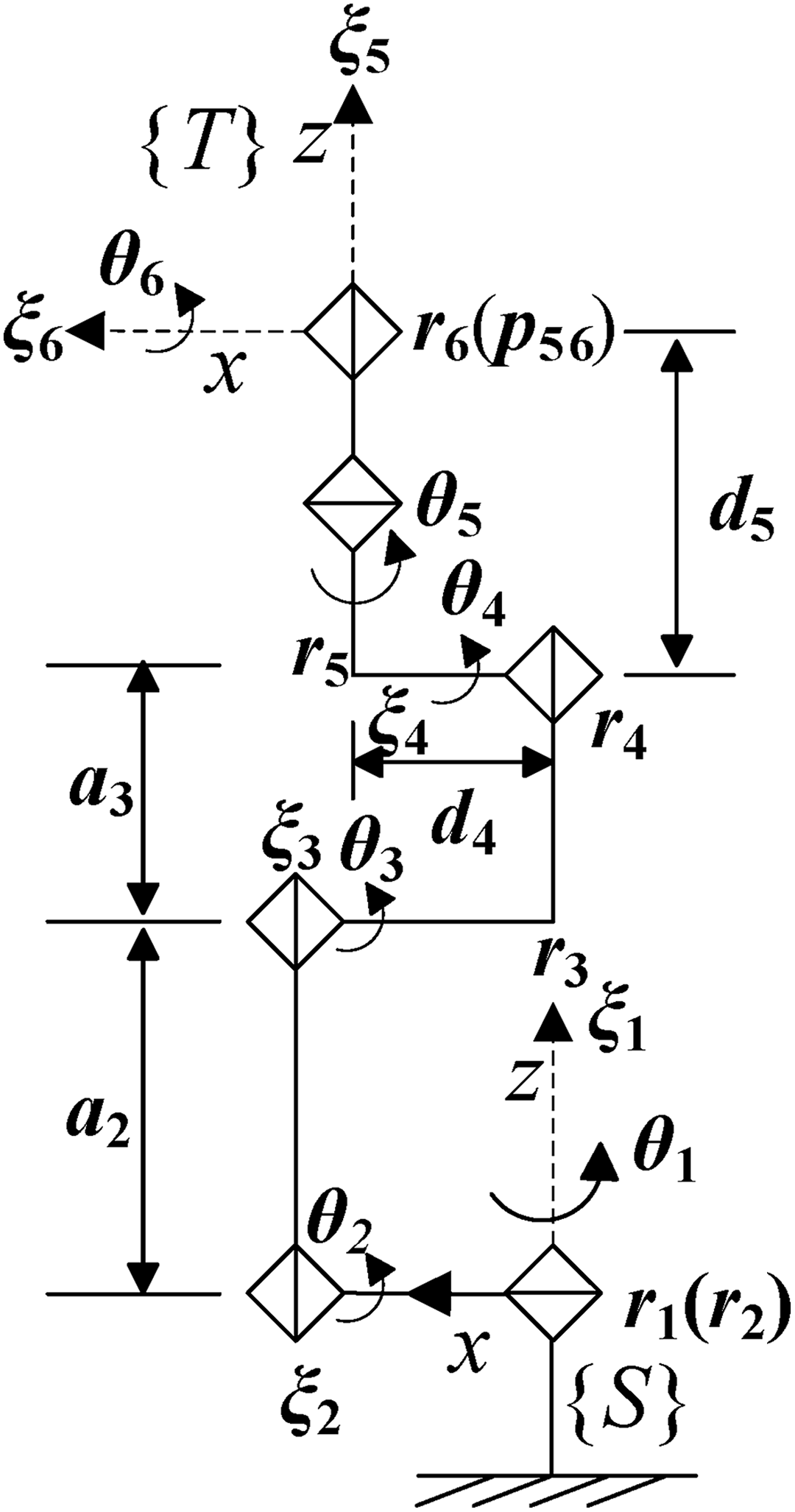
Structure coordinates.

Table 1.

D-H parameters of OUR-1 robot.

Joint no.	θi (°)	di (mm)	ai (mm)	αi (°)	Joint range 35 (°)
1	θ 1	0	0	90	(−180, 180)
2	θ 2	0	427	0	(−180, 180)
3	θ 3	0	328.5	0	(−180, 180)
4	θ 4	116.5	0	−90	(−180, 180)
5	θ 5	116.5	0	90	(−180, 180)
6	θ 6	0	0	0	(−180, 180)

D-H: Denavit–Hatenberg.

The unit vector ω_i , point r_i , and twist ξ_i of each joint are constructed as follows

$\begin{array}{l}{\omega }_1=\left[\begin{array}{c}0\\ 0\\ 1\end{array}\right],{\omega }_2=\left[\begin{array}{c}1\\ 0\\ 0\end{array}\right],{\omega }_3=\left[\begin{array}{c}1\\ 0\\ 0\end{array}\right],{\omega }_4=\left[\begin{array}{c}1\\ 0\\ 0\end{array}\right],{\omega }_5=\left[\begin{array}{c}0\\ 0\\ 1\end{array}\right],{\omega }_6=\left[\begin{array}{c}1\\ 0\\ 0\end{array}\right]\\ r_1=r_2=\left[\begin{array}{c}0\\ 0\\ 0\end{array}\right],r_3=\left[\begin{array}{c}0\\ 0\\ a_2\end{array}\right],r_4=\left[\begin{array}{c}0\\ 0\\ a_2+a_3\end{array}\right],r_5=\left[\begin{array}{c}{d}_4\\ 0\\ a_2+a_3\end{array}\right],r_6=\left[\begin{array}{c}{d}_4\\ 0\\ a_2+a_3+d_5\end{array}\right]\\ {\xi }_1=\left[\begin{array}{c}0\\ 0\\ 1\\ 0\\ 0\\ 0\end{array}\right],{\xi }_2=\left[\begin{array}{c}1\\ 0\\ 0\\ 0\\ 0\\ 0\end{array}\right],{\xi }_3=\left[\begin{array}{c}1\\ 0\\ 0\\ 0\\ a_2\\ 0\end{array}\right],{\xi }_4=\left[\begin{array}{c}1\\ 0\\ 0\\ 0\\ a_2+a_3\\ 0\end{array}\right],{\xi }_5=\left[\begin{array}{c}0\\ 0\\ 1\\ 0\\ -d_4\\ 0\end{array}\right],{\xi }_6=\left[\begin{array}{c}1\\ 0\\ 0\\ 0\\ a_2+a_3+d_5\\ 0\end{array}\right]\end{array}$

We can represent the initial configuration in Figures 1 and 4 by

$g_{st}(0)=\left[\begin{array}{cccc}1& 0& 0& d_4\\ 0& 1& 0& 0\\ 0& 0& 1& a_2+a_3+d_5\\ 0& 0& 0& 1\end{array}\right]$

9

The configuration of the 6-DOF serial robots is expressed by the POE formula of the forward kinematics as follows

$g_{st}(\theta )=e^{{\widehat{\xi }}_1{\theta }_1}{e}^{{\widehat{\xi }}_2{\theta }_2}{e}^{{\widehat{\xi }}_3{\theta }_3}{e}^{{\widehat{\xi }}_4{\theta }_4}{e}^{{\widehat{\xi }}_5{\theta }_5}{e}^{{\widehat{\xi }}_6{\theta }_6}{g}_{st}(0)$

10

$\begin{array}{l}\text{where} e^{{\widehat{\xi }}_1{\theta }_1}=\left[\begin{array}{cccc}\text{cos}{\theta }_1& -\text{sin}{\theta }_1& 0& 0\\ \text{sin}{\theta }_1& \text{cos}{\theta }_1& 0& 0\\ 0& 0& 1& 0\\ 0& 0& 0& 1\end{array}\right],e^{{\widehat{\xi }}_2{\theta }_2}=\left[\begin{array}{cccc}1& 0& 0& 0\\ 0& \text{cos}{\theta }_2& -\text{sin}{\theta }_2& 0\\ 0& \text{sin}{\theta }_2& \text{cos}{\theta }_2& 0\\ 0& 0& 0& 1\end{array}\right]\\ e^{{\widehat{\xi }}_3{\theta }_3}=\left[\begin{array}{cccc}1& 0& 0& 0\\ 0& \text{cos}{\theta }_3& -\text{sin}{\theta }_3& a\text{sin}{\theta }_3\\ 0& \text{sin}{\theta }_3& \text{cos}{\theta }_3& -a_2(\text{cos}{\theta }_3-1)\\ 0& 0& 0& 1\end{array}\right],e^{{\widehat{\xi }}_4{\theta }_4}=\left[\begin{array}{cccc}1& 0& 0& 0\\ 0& \text{cos}{\theta }_4& -\text{sin}{\theta }_4& (a_2+a_3)\text{sin}{\theta }_4\\ 0& \text{sin}{\theta }_4& \text{cos}{\theta }_4& -(a_2+a_3)(\text{cos}{\theta }_4-1)\\ 0& 0& 0& 1\end{array}\right]\\ e^{{\widehat{\xi }}_5{\theta }_5}=\left[\begin{array}{cccc}\text{cos}{\theta }_5& -\text{sin}{\theta }_5& 0& -d_4(\text{cos}{\theta }_5-1)\\ \text{sin}{\theta }_5& \text{cos}{\theta }_5& 0& -d_4\text{sin}{\theta }_5\\ 0& 0& 1& 0\\ 0& 0& 0& 1\end{array}\right],e^{{\widehat{\xi }}_6{\theta }_6}=\left[\begin{array}{cccc}1& 0& 0& 0\\ 0& \text{cos}{\theta }_6& -\text{sin}{\theta }_6& (a_2+a_3+d_5)\text{sin}{\theta }_6\\ 0& \text{sin}{\theta }_6& \text{cos}{\theta }_6& (a_2+a_3+d_5)(1-\text{cos}{\theta }_6)\\ 0& 0& 0& 1\end{array}\right]\end{array}$

Solving the inverse kinematics

Solving θ ₁

Suppose that ξ ₁, ξ ₂, ξ ₃, and ξ ₄ are unit twists with zero-pitch. Right-multiplying equation (10) by g_st ⁻¹ (0) obtains

$g_{st}(\theta )g_{st}{ }^{-1}(0)=e^{{\widehat{\xi }}_1{\theta }_1}{e}^{{\widehat{\xi }}_2{\theta }_2}{e}^{{\widehat{\xi }}_3{\theta }_3}{e}^{{\widehat{\xi }}_4{\theta }_4}{e}^{{\widehat{\xi }}_5{\theta }_5}{e}^{{\widehat{\xi }}_6{\theta }_6}=g_{st1}$

11

Assume that the axes of the fifth and sixth joints intersect at point p ₅₆. Right-multiplying equation (11) by p ₅₆, and according to the principle of position invariance, we can get

$g_{st1}\cdot p_{56}=e^{{\widehat{\xi }}_1{\theta }_1}{e}^{{\widehat{\xi }}_2{\theta }_2}{e}^{{\widehat{\xi }}_3{\theta }_3}{e}^{{\widehat{\xi }}_4{\theta }_4}{p}_{56}=p_1={(p_x,p_y,p_z,1)}^T$

12

The equation (12) represents the screw motion of point p ₅₆ in the first four joints and corresponds to the geometrical graph, as shown in Figure 5.

Figure 5.

The screw motion of the first four joints.

As illustrated in Figure 5, point p ₅₆ first of all reaches point p ₄ by rotating angle θ ₄ around axis ξ ₄. This point then reaches point p ₃ by rotating angle θ ₃ around axis ξ ₃. After that, point p ₃ reaches point p ₂ by rotating angle θ ₂ around axis ξ ₂, and finally reaches point p ₁ by rotating angle θ ₁ around axis ξ ₁ in the initial configuration. The key to solving angle θ ₁ is to calculate point p ₂. This point can be determined by the known point p ₅₆ and p ₁.

According to the geometrical relationship in Figure 5, we have

$\{\begin{array}{c}(p_2-p_{56})\cdot {\omega }_2=0\\ (p_2-o_1)\cdot {\omega }_1=0\\ \Vert p_2-o_1\Vert =\Vert p_1-o_1\Vert \end{array}$

13

where ω ₁, ω ₂, o ₁, and p ₅₆ are represented as follows

${\omega }_1=\left[\begin{array}{c}0\\ 0\\ 1\end{array}\right],{\omega }_2=\left[\begin{array}{c}1\\ 0\\ 0\end{array}\right],o_1=\left[\begin{array}{c}1\\ 0\\ p_z\end{array}\right],p_{56}=\left[\begin{array}{c}{d}_4\\ 0\\ a_2+a_3+d_5\end{array}\right].$

Point p ₂ can be obtained using equation (13)

$p_2={(d_4,\pm \sqrt{p_x{ }^2+p_y{ }^2-d_4{ }^2},p_z)}^T$

14

The screw motion in the first joint can be expressed as

$e^{{\widehat{\xi }}_1{\theta }_1}\cdot p_2=p_1$

15

Adopting the Paden–Kahan subproblem 1 ² , the θ ₁ can be given as follows

${\theta }_1=a\text{tan}2(-p_x(\pm s_1)+d_4{p}_y,d_4{p}_x\pm p_y{s}_1)$

16

where $s_1=\sqrt{p_x{ }^2+p_y{ }^2-d_4{ }^2}$ .

Solving θ ₅ and θ ₆

Left-multiplying equation (11) by $e^{-{\widehat{\xi }}_1{\theta }_1}$ gives

$e^{-{\widehat{\xi }}_1{\theta }_1}\cdot g_{st1}=e^{{\widehat{\xi }}_2{\theta }_2}{e}^{{\widehat{\xi }}_3{\theta }_3}{e}^{{\widehat{\xi }}_4{\theta }_4}{e}^{{\widehat{\xi }}_5{\theta }_5}{e}^{{\widehat{\xi }}_6{\theta }_6}$

17

Let $e^{{\widehat{\xi }}_2{\theta }_2}{e}^{{\widehat{\xi }}_3{\theta }_3}{e}^{{\widehat{\xi }}_4{\theta }_4}{e}^{{\widehat{\xi }}_5{\theta }_5}{e}^{{\widehat{\xi }}_6{\theta }_6}=g_{st2}$

In equation (10), let

$g_{st}(\theta )=\left[\begin{array}{cccc}{M}_1& N_1& G_1& H_1\\ M_2& N_2& G_2& H_2\\ M_3& N_3& G_3& H_3\\ 0& 0& 0& 1\end{array}\right]$

18

Then, the $g_{st1}=g_{st}(\theta )g_{st}{ }^{-1}(0)$ .

According to the corresponding matrix elements of each side in equation (17), the equation set can be obtained

$\{\begin{array}{c}\text{cos}{\theta }_5=M_1\text{cos}{\theta }_1+M_2\text{sin}{\theta }_1\\ \text{sin}{\theta }_5\text{sin}{\theta }_6=G_1\text{cos}{\theta }_1+G_2\text{sin}{\theta }_1\\ -\text{sin}{\theta }_5\text{cos}{\theta }_6=N_1\text{cos}{\theta }_1+N_2\text{sin}{\theta }_1\\ \text{sin}{\theta }_5\text{sin}({\theta }_2+{\theta }_3+{\theta }_4)=M_3\\ \text{sin}{\theta }_5\text{cos}({\theta }_2+{\theta }_3+{\theta }_4)=M_2\text{cos}{\theta }_1-M_1\text{sin}{\theta }_1\end{array}$

19

The θ ₅, θ ₆, and (θ ₂ + θ ₃ + θ ₄) can be determined by utilizing equation (19)

${\theta }_5=a\text{tan}2(\pm \sqrt{1-s_2{ }^2},s_2)$

20

${\theta }_6=a\text{tan}2(s_3/\text{sin}{\theta }_5,-s_4/\text{sin}{\theta }_5)\begin{array}{c} \end{array}(\text{sin}{\theta }_5\ne 0)$

21

${\theta }_2+{\theta }_3+{\theta }_4=a\text{tan}2(M_3/\text{sin}{\theta }_5,s_5/\text{sin}{\theta }_5)\begin{array}{c} \end{array}(\text{sin}{\theta }_5\ne 0)$

22

where $s_2=M_1\text{cos}{\theta }_1+M_2\text{sin}{\theta }_1,s_3=G_1\text{cos}{\theta }_1+G_2\text{sin}{\theta }_1,s_4=N_1\text{cos}{\theta }_1+N_2\text{sin}{\theta }_1,$ $s_5=M_2\text{cos}{\theta }_1-M_1\text{sin}{\theta }_1.$

Solving θ ₂, θ ₃, and θ ₄

Right-multiplying equation (17) by $e^{-}{ }^{{\widehat{\xi }}_6{\theta }_6}$ , $e^{-}{ }^{{\widehat{\xi }}_5{\theta }_5}$ respectively, gives

$g_{st2}\cdot e^{-{\widehat{\xi }}_6{\theta }_6}{e}^{-{\widehat{\xi }}_5{\theta }_5}=e^{{\widehat{\xi }}_2{\theta }_2}{e}^{{\widehat{\xi }}_3{\theta }_3}{e}^{{\widehat{\xi }}_4{\theta }_4}$

23

Let $e^{{\widehat{\xi }}_2{\theta }_2}{e}^{{\widehat{\xi }}_3{\theta }_3}{e}^{{\widehat{\xi }}_4{\theta }_4}=g_{st3}$ and it can be expressed as follows

$g_{st3}=\left[\begin{array}{cccc}{m}_1& n_1& g_1& t_4\\ m_2& n_2& g_2& t_5\\ m_3& n_3& g_3& t_6\\ 0& 0& 0& 1\end{array}\right]$

24

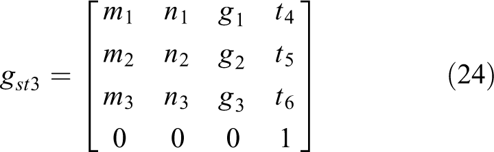
From equations (23) and (24), we can obtain

$\{\begin{array}{c}-a_3\text{sin}({\theta }_2+{\theta }_3)-a_2\text{sin}{\theta }_2=t_7\\ a_3\text{cos}({\theta }_2+{\theta }_3)+a_2\text{cos}{\theta }_2=t_8\end{array}$

25

where $t_7=t_5-\left(a_2+a_3\right)\text{sin}\left({\theta }_2+{\theta }_3+{\theta }_4\right),t_8=t_6+\left(a_2+a_3\right)\text{cos}\left({\theta }_2+{\theta }_3+{\theta }_4\right)$ .

The θ ₂ and (θ ₂ + θ ₃) can be given according to equation (25).

${\theta }_2=a\text{tan}2(B,A)+a\text{tan}2(C,\pm \sqrt{A^2+B^2-C^2})$

26

${\theta }_2+{\theta }_3=a\text{tan}2(-s_6/a_3,s_7/a_3)$

27

where $A=2a_2{t}_7,B=2a_2{t}_8,C=a_3{ }^2-a_2{ }^2-t_7{ }^2-t_8{ }^2,s_6=a_2\text{sin}{\theta }_2+t_7,s_7=t_8-a_2\text{cos}{\theta }_2$ .

We can determine θ ₃ and θ ₄ by

${\theta }_3=({\theta }_2+{\theta }_3)-{\theta }_2$

28

${\theta }_4=({\theta }_2+{\theta }_3+{\theta }_4)-({\theta }_2+{\theta }_3)$

29

Until now, the closed solutions of inverse kinematics have been determined completely by applying Paden–Kahan subproblem and the matrix theory. The algorithm of inverse kinematics proposed in this article is applicable to 6-DOF robots with only rotational joints, such as OUR robots, UR robots, or other robots with the similar structure. It is worth mentioning that the calculation can be greatly simplified if we choose a suitable reference coordinate frame such as the inertial coordinate frame {S}.

Experiment and verification

The inverse kinematic solution of OUR-1 robot is calculated in order to verify the correctness of the proposed algorithm. The structure parameters of OUR-1 robot as shown in Table 1 are

$a_2=427\text{mm},a_3=328.5\text{mm},d_4=116.5\text{mm},d_5=116.5\text{mm}$

30

In the process of validating the algorithm of inverse kinematics, a set of initial angles are firstly selected within the range of joint motion, and the target pose is calculated by the POE formula. Then, according to the obtained pose and the proposed algorithm, the angle of each joint is determined. After that, we use the obtained sets of angles again to solve the target pose. Both of the forward and inverse kinematics of robots are computed by utilizing MATLAB. The specific validation procedure is presented as follows:

Step 1: Arbitrarily choose a group of joint angles within the workspace.

${\theta }_1=60,{\theta }_2=30,{\theta }_3=-50,{\theta }_4=150,{\theta }_5=20,{\theta }_6=-100$

31

Step 2: Solve the forward kinematics to obtain the pose of the end effector adopting equation (10)

$g_{st}(\theta )=\left[\begin{array}{cccc}0.66023880& -0.71447481& 0.23153935& 223.13306207\\ 0.70387453& 0.48108125& -0.52261026& 5.69667927\\ 0.26200263& 0.50802222& 0.82052912& 603.59711682\\ 0& 0& 0& 1\end{array}\right]$

32

Step 3: Solve the inverse kinematics to get all possible joint angles according to the proposed method and the pose obtained above.

The eight groups of solutions of inverse kinematics are given as shown in Table 2. As illustrated in Table 2, the fifth group of joint angles is exactly the same as the angles given in step 1 under the condition of reserving to twelve decimal places.

Table 2.

Eight solutions of inverse kinematics.

No.	θ 1/(°)	θ 2/(°)	θ 3/(°)	θ 4/(°)	θ 5/(°)	θ 6/(°)
1	−57.075065532537	13.250529664305	−89.914814615889	92.289797959018	103.412170716869	35.475115065932
2	−57.075065532537	−61.829778895480	89.914814615889	−12.459522712973	103.412170716869	35.475115065932
3	−57.075065532537	−0.330428295745	−28.130335134466	−135.913723562355	−103.412170716869	−144.524884934068
4	−57.075065532537	−24.719046700937	28.130335134466	−167.785775426094	−103.412170716869	−144.524884934068
5	60.000000000000	30.000000000000	−50.000000000000	150.000000000000	20.000000000000	−100.000000000000
6	60.000000000000	−13.041867066974	50.000000000000	93.041867066974	20.000000000000	−100.000000000000
7	60.000000000000	60.089523137324	−76.079430396494	−34.010092740830	−20.000000000000	80.000000000000
8	60.000000000000	−4.341004598576	76.079430396494	−121.738425797918	−20.000000000000	80.000000000000

Step 4: Solve the forward kinematics again to get the corresponding poses of the eight solutions mentioned above.

Step 5: Calculate the 2-norm of the difference matrix between steps 2 and 4 and find out the maximal pose error.

By comparison, the 2-norm of the difference matrix of the fourth group of solutions is maximal, as follows

${\text{norm}}_4=3.770565865534826\times {10}^{-13}$

33

The corresponding maximal error of pose $\Delta g_{\text{max}}$ is given as follows

$\begin{array}{c}\Delta g_{\text{max}}=g_{st}-g_{st4}={10}^{-12}\times \left[\begin{array}{cccc}0.00033307& 0.00022204& 0.00000000& -0.11368684\\ -0.00011102& 0.00016653& -0.00022204& -0.11368684\\ 0.00005551& 0.00011102& -0.00011102& 0.34106051\\ 0.00000000& 0.00000000& 0.00000000& 0.00000000\end{array}\right]\end{array}$

34

where g_st and g_{st 4} are the corresponding poses of the given group and the fourth group of joint angles, respectively.

In the experiment, a group of closed solutions, that is, eight solutions are determined because the three adjacent joint axes of OUR-1 robots are parallel to each other. From the proposed algorithm and the results of inverse kinematics as illustrated in Table 2, we can see that special features of the closed form solution are presented: the angles θ ₁, θ ₅, θ ₆ of the first and second groups, the third and fourth groups, the fifth and sixth groups, the seventh and eighth groups of solutions are same respectively, and the sum of angle θ ₂, θ ₃, and θ ₄ of every two groups are also the same, which are generated by the special structure of the robot. To verify the correctness of the algorithm of inverse kinematics, we compare the obtained eight sets of solutions with the given set of angles and find that the fifth set of solution is exactly the same as the given angles. In addition, we also calculate the difference of matrix between the corresponding pose of eight sets of solutions and the given pose and solve the 2-norm of each difference of matrix, which represents the size of the distance of error matrix, and the larger the 2-norm, the greater the error. Finally, the maximal 2-norm of the difference of matrix is in the order of 10⁻¹³ magnitude as shown in equation (33), and the corresponding maximal pose error is in the order of 10⁻¹² magnitude as presented in equation (34), which verifies the correctness and high precision of the algorithm.

Example analysis of kinematic model

In “Screw theory of rigid bodies and model analysis” section, the parameter singularity of the D-H and POE models is discussed and in this section, we will analyze the two models in combination with OUR-1 robots.

As shown in Figure 1, the second, third, and fourth joint axes of OUR-1 robot are parallel. Assume that the structure of OUR-1 robot has no errors except for the third joint axis having a slight deviation angle γ with respect to the parallel axes and the first three joint coordinate frames of OUR-1 robot employing the D-H modeling method, as shown in Figure 6. When the second and third joint axes are parallel, the D-H parameters of the second link are θ = 90°, d = 0, a = a ₂, α = 0, while they become θ = 0, d = −d ₂′, a = 0, α = −γ when the third joint axis has a deviation angle γ. Given the above mentioned situation, the D-H parameters vary greatly with a small error from the orientation of the parallel joint axes. It’s worth mentioning that parameter d = −a ₂cot(γ) → ∞ when γ → 0. Namely, the distance d changes sensitively and jumps rapidly when γ → 0. Hence, the parameters of this model are discontinuous leading to the singularity of the model when the adjacent joints have parallel or close to parallel axes.

Figure 6.

The first three joint coordinate frames.

Similarly, suppose that the structure of OUR-1 robot has no deviations except for the third joint axis having an error angle γ relative to the parallel axes. To better demonstrate that the POE-based model is singularity-free, here we might as well assume that the absolute value of angle γ is within 5° and that the twist of the third joint is ξ ₃ = (ω ₃;ν ₃), where ω ₃ = [ω_x , ω_y , ω_z ] ^T and υ ₃ = [υ_x , υ_y , υ_z ] ^T . The POE method is adopted for kinematics modeling. When the third joint axis has a deviation angle γ with respect to the parallel axes, the error of twist ξ ₃ is calculated by sampling 21 points at equal intervals, as shown in Figure 7. From Figure 7, the errors of twist ξ ₃ vary slowly and smoothly with slight changes from the parallel joint axes. That is to say, the slight deviation from the parallel joint axes can be described by the small changes in the kinematic parameters. The actual parameters of this model can be identified in the kinematic calibration. Therefore, it would be helpful to illustrate that the POE-based model is singularity-free.

Figure 7.

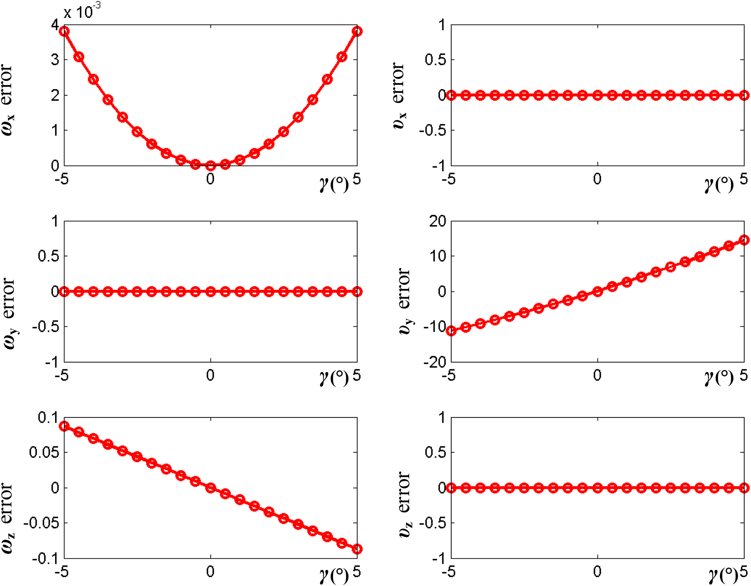
Error results.

Conclusion

The inverse kinematics of the OUR-1 robot is solved by employing the analytical, geometric, and algebraic methods combined with the Paden–Kahan subproblem as well as matrix theory. Clear geometric significance is presented by applying the geometric method. The kinematic parameters of the D-H and the POE-based models are analyzed and illustrated to demonstrate the problem of singularity of the two models. The singularity of the model depends on whether the kinematic parameters are continuous. If they are continuous, the model is nonsingular; otherwise, it is singular. In experiments, we obtain eight solutions of inverse kinematics, and the correctness and high level of accuracy of the proposed algorithm are verified by calculating the maximal 2-norm of the difference matrix and the corresponding pose error of OUR-1 robot, which is in the order of 10⁻¹² magnitude. This algorithm utilizes the motion trajectory of screw as illustrated in Figure 5, which can make the geometric significance clearer and be applied to the 6R serial robots with the similar structure to OUR robots or UR robots. In future work, robot kinematics calibration, the selection of optimal solution and trajectory planning need to be further studied.