Algorithmic approach to geometric solution of generalized Paden–Kahan subproblem and its extension

Abstract

Kinematics as a science of geometry of motion describes motion by means of position, orientation, and their time derivatives. The focus of this article aims screw theory approach for the solution of inverse kinematics problem. The kinematic elements are mathematically assembled through screw theory by using only the base, tool, and workpiece coordinate systems—opposite to conventional Denavit–Hartenberg approach, where at least n + 1 coordinate frames are needed for a robot manipulator with n joints. The inverse kinematics solution in Denavit–Hartenberg convention is implicit. Instead, explicit solutions to inverse kinematics using the Paden–Kahan subproblems could be expressed. This article gives step-by-step application of geometric algorithm for the solution of all the cases of Paden–Kahan subproblem 2 and some extension of that subproblem based on subproblem 2. The algorithm described here covers all of the cases that can appear in the generalized subproblem 2 definition, which makes it applicable for multiple movement configurations. The extended subproblem is used to solve inverse kinematics of a manipulator that cannot be solved using only three basic Paden–Kahan subproblems, as they are originally formulated. Instead, here is provided solution for the case of three subsequent rotations, where last two axes are parallel and the first one does not lie in the same plane with neither of the other axes. Since the inverse kinematics problem may have no solution, unique solution, or many solutions, this article gives a thorough discussion about the necessary conditions for the existence and number of solutions.

Introduction

Historically, fundamental Chasles’ theorem states that every proper motion is given by screw motion. Proper motion is three-dimensional (3-D) rotation about arbitrary axis followed by 3-D translation and describes the rigid body motion. A screw motion is rotation about arbitrary axis, followed by translation along the same axis. Formulation and proof using modern mathematical language is given by Palais and Palais ¹ and in more depth and details by Selig. ²

If the set of geometrical characteristics is given, the position and orientation of every link of the robot could be expressed as function of the joint variables. A chain of coordinate systems is attached to the joints using traditional Denavit–Hartenberg (DH) convention, originally established in the study by Denavit and Hartenberg. ³ They are related by 4 × 4 matrices used to describe rigid body motion. Details for DH convention and non-DH method discussion and introduction to screw theory, are given in the study by Jazar, ⁴ as well.

The most comprehensive and exact approach to build the screw theory and its application in robotics is given by Murray et al. ⁵

Rotation about direction specified with the unit vector $\omega \in {\Re }^3$ and angle θ is represented by 3 × 3 matrix, given in exponential form

$e^{\widehat{\omega }\theta }=I_3+\widehat{\omega }\text{sin }\theta +\widehat{\omega }\left(1-\text{cos}\theta \right)$

1

Equation (1) also is known as Rodrigues formula and its exponential form gives efficient computing method. I ₃ is the identity matrix of order 3 and $\widehat{\omega }$ is the skew-symmetric matrix obtained of coordinates of the vector $\omega ={\left[\begin{array}{ccc}{\omega }_1& {\omega }_2& {\omega }_3\end{array}\right]}^T$

$\widehat{\omega }=\left[\begin{array}{ccc}0& -{\omega }_3& {\omega }_2\\ {\omega }_3& 0& -{\omega }_1\\ -{\omega }_2& {\omega }_1& 0\end{array}\right]$

2

Let $v,\omega \in {\Re }^3$ are unit vectors in 3-D. A twist coordinates ξ are determined as

$\xi =\left[\begin{array}{c}v\\ \omega \end{array}\right]\in {\Re }^6$

3

and a twist $\widehat{\xi }$ is defined as 4 × 4 matrix

$\widehat{\xi }=\left[\begin{array}{cc}\widehat{\omega }& v\\ 0& 0\end{array}\right]$

4

A screw motion consists of rotation about an axis in direction determined by the unit vector ω, through an angle θ followed by translation by an amount d along the same axis. If it is not pure translation, then θ ≠ 0, so a pitch of the screw could be defined as h =d/θ. Let q be the arbitrary point of the axis of the screw. In a case of general screw motion which is not pure translation, the vector

$v=-\omega \times q+h\omega$

5

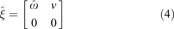
determines the twist coordinates, equation (3) and as well the twist, equation (4). This screw motion is represented by 4 × 4 matrix, denoted as exponential of $\widehat{\xi }\theta$

$e^{\widehat{\xi }\theta }=\left[\begin{array}{cc}{e}^{\widehat{\omega }\theta }& \left(I_3-e^{\widehat{\omega }\theta }\right)\left(\omega \times v\right)+\omega {\omega }^{T}v\theta \\ 0& 1\end{array}\right]$

6

The pure rotation as special case of screw motion with pitch h = 0 is represented by equation (6) as well, taking the twist coordinates to be

$\xi =\left[\begin{array}{c}-\omega \times q\\ \omega \end{array}\right]$

7

In the case of pure translation in a direction determined by unit vector v by amount θ, the twist is defined as

$\xi =\left[\begin{array}{c}v\\ 0\end{array}\right]$

8

and its exponential form is given by

$e^{\widehat{\xi }\theta }=\left[\begin{array}{cc}{I}_3& v\theta \\ 0& 1\end{array}\right]$

9

Robot manipulator consists of sequence of rigid links, connected by joints with motors attached on them. Robot manipulator with n joints is said to have n degrees of freedom (DOF). The motion for every joint is determined with three constant parameters and one variable. All the n variables of the joints form the machine space (joint space) of the robot manipulator. The machine coordinates of the manipulator of n DOF are

$\theta ={\left[\begin{array}{ccc}{\theta }_1& {\theta }_2\dots & {\theta }_n\end{array}\right]}^T$

10

The end effector of the robot manipulator is needed to be controlled in the sense to control its pose—position and orientation. That determines the pose space of the robot manipulator.

Forward kinematics is a procedure for obtaining the pose of the robot manipulator if the machine coordinates are given. More formally, forward kinematics is a function from machine space to pose space of the robot.

Using screw theory, the forward kinematics is determined as product of the exponentials of the appropriate twists for each link, respectively

$g\left(\theta \right)=e^{{\widehat{\xi }}_1{\theta }_1}{e}^{{\widehat{\xi }}_2{\theta }_2}\mathrm{...}{e}^{{\widehat{\xi }}_n{\theta }_n}$

11

Only two coordinate frames are sufficient—the tool and base frame. If g_bt(0) is the transformation matrix from tool to base coordinate frame when all machine coordinates are zeros, the forward kinematics map is determined by

$g_{bt}\left(\theta \right)=g\left(\theta \right)g_{bt}\left(0\right)=e^{{\widehat{\xi }}_1{\theta }_1}{e}^{{\widehat{\xi }}_2{\theta }_2}\mathrm{...}{e}^{{\widehat{\xi }}_n{\theta }_n}{g}_{bt}\left(0\right)$

12

Some robotized machines are configured with two kinematics chains. Forward and inverse kinematics can be solved in similar manner. ⁶ Xiang and Altintas ⁶ give comparison between DH approach against screw theory approach. The latter is better since no local coordinate systems are needed and it provides explicit solution to the inverse kinematics problem. ⁷ Details and different inverse kinematic formulation methods for industrial robot manipulators using screw theory could be found in the study by Sariyildiz et al. ⁸ Comparison between both methods is given by Rocha et al. ⁹

If the pose coordinates of the end effector are given, inverse kinematics problem is used to find the machine coordinates. Inverse kinematics problem may have no solution, unique solution, or many solutions. Standard approach, using DH convention is focused on solving equation systems and optimization techniques in some cases.

We prefer screw theory, especially the geometric algorithm approach explained in this article, over the traditional DH method. There are several advantages

In DH convention at least n + 1 coordinate frames are needed, since a robot manipulator with n joints will have n + 1 links, and we rigidly attach a coordinate frame to each link. ¹⁰

The choice for a coordinate frames in DH convention is constrained by the DH coordinate frame assumptions, so a procedure for assigning coordinate frames that satisfy the constraints is needed to be performed. ¹⁰

In screw theory, often, only two coordinate frames are sufficient, the base frame, and the tool frame, so it is more simple to explain entire kinematic chain. ⁵

Given the DH parameters for a manipulator, the corresponding twists can be easily determined. ⁵

The inverse kinematics solution in DH convention is implicit. Using screw theory, it is possible to find explicit solutions to inverse kinematics using the Paden–Kahan subproblems or its extensions. ⁷

The screw theory offers way to express explicit solution that can be reduced to an application of geometric algorithm. There are many researches and case studies based on screw theory published in the last decade. ^{11 –18}

For a large number of robot manipulators, it is sufficient to implement three classical Paden–Kahan subproblems, originally established in the study by Paden. ¹⁹

Paden–Kahan subproblems

The most commonly used geometric algorithms in inverse kinematics problem solutions are addressed by Murray et al. ⁵

Subproblem 1

Let ξ be a zero-pitch twist with unit magnitude and $p,q\in {\Re }^3$ two points. Find θ such that

$e^{\widehat{\xi }\theta }p=q$

13

Subproblem 2

Let ξ₁ and ξ₂ be two zero-pitch twists with unit magnitudes with intersecting axes and $p,q\in {\Re }^3$ two points. Find θ₁ and θ₂ such that

$e^{{\widehat{\xi }}_1{\theta }_1}{e}^{{\widehat{\xi }}_2{\theta }_2}p=q$

14

Subproblem 3

Let ξ be a zero-pitch twist with unit magnitude, $p,q\in {\Re }^3$ two points and δ positive real number. Find θ such that

$\Vert q-p{e}^{\widehat{\xi }\theta }\Vert =\delta$

15

All subproblems stated this way are completely solved in the study by Murray et al. ⁵ There are also several examples of robot manipulators and the inverse kinematics problem solutions based on reducing the full inverse kinematics problem into appropriate subproblems.

There exist robot manipulators that cannot be solved using only these three such formulated subproblems. The study of Yew-sheng and Ai-ping ²⁰ gives example of 5-DOF manipulator with two consequent nonintersecting rotational axes. They have changed the condition for existing intersection point of the axes in subproblem 2. The new subproblem is formulated and the complete solution for nonintersecting axes is fully explained in the study by Yew-sheng and Ai-ping. ²⁰

Generalization of subproblem 2

From mathematical point of view, subproblems considered in the studies by Murray et al. ⁵ and Yew-sheng and Ai-ping ²⁰ are just cases of one general subproblem. All of the cases can be covered considering the generalized formulation as it follows.

Subproblem 2 (generalized)

Let ξ₁ and ξ₂ be two zero-pitch twists with unit magnitudes and $p,q\in {\Re }^3$ two points. Find θ₁ and θ₂, so that the equation (14) is satisfied.

Solution

Geometrically, the problem is to find the angles θ₁ and θ₂, so then if the point p is rotated about axis of the twist ξ₂ by the angle θ₂ and then is rotated about axis of the twist ξ₁ by the angle θ₁, it will coincident with the point q.

Let ω₁ and ω₂ be the unit vectors in a direction of the axes of the twists ξ₁ and ξ₂, respectively. In general, there are four cases (two cases by two subcases), on dependence on relative position of the axes in the space.

Case 1

ω₁ × ω₂ ≠ o: axes of rotation intersect in exactly one point or they are skew lines.

Case 1a

The axes of rotation intersect in exactly one point r. This is the case completely solved in the study by Murray et al., ⁵ but necessary conditions for solution are just mentioned in passing.

Case 1b

The axes of rotation are skew lines. This is the case solved in the study by Yew-sheng and Ai-ping, ²⁰ but discussion for existence of the solution and number of solutions is purely mentioned.

Below is given a new geometrical solution that covers the both subcases—cases 1a and 1b with detailed discussion about the existence of a solution and the number of solutions. This new algorithmic approach of geometrical solution consists of five steps detailed below. In fact, this solution is described as geometric algorithm and its steps refer to well-known geometric algorithms. Most of them have good explanation in the study by Dunn and Parberry. ²¹

Step 1

Determine the closest points r ₁ and r ₂ between the axes of twists ξ₁ and ξ₂.

In the case where the two axes intersect in exactly one point, the closest point between them will be the intersecting point, and r ₁ = r ₂ = r. So, all the equations given in this section will be valid as well for the both subcases.

Step 2

Determine plane ∑₁, the plane that is normal to the unit vector ω₁ and passes through the point q (plane of the red circle—Figure 1). Determine plane ∑₂, the plane that is normal to the unit vector ω₂ and passes through the point p (plane of the blue circle—Figure 1). Next, determine the intersecting line l(t) of these two planes ∑₁ and ∑₂

$l\left(t\right)=l_0+t\cdot D$

16

where l ₀ is an arbitrary point of line l(t) and D is unit vector in direction of line l(t).

Figure 1.

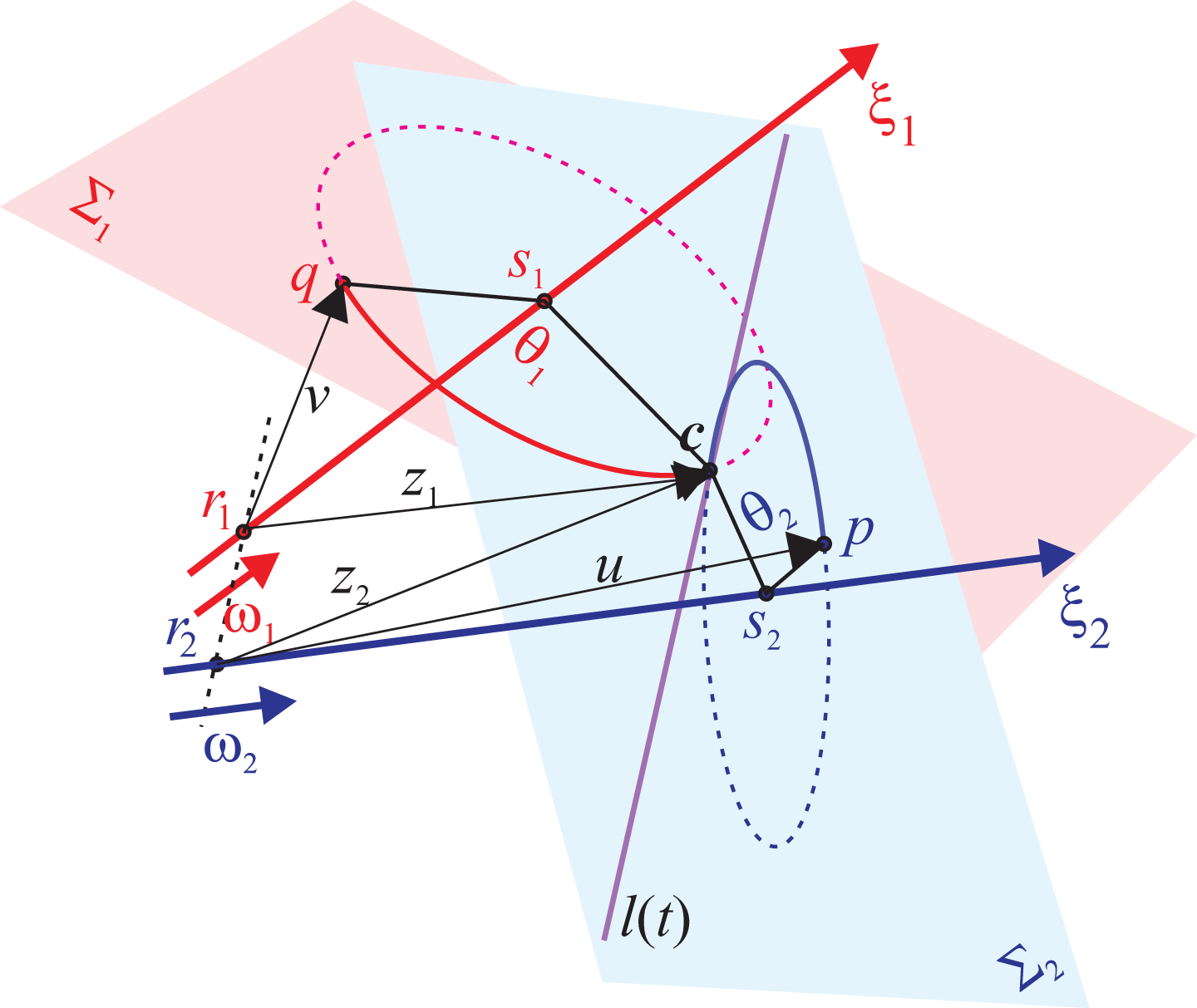
Geometry representation of the solution to generalized subproblem 2 case: ω₁ × ω₂ ≠ o

Step 3

Use the point r ₁ to determine the projection s ₁ of the point q on the axis of the twist ξ₁

$s_1=r_1+{\omega }_1\left({\omega }_1{\hspace{0.17em}}^{T}v\right)$

17

where v = q − r₁.

Determine the intersection between the line l(t) and the red circle, circle k ₁ centered in point s ₁ and radius R ₁

$R_1=\Vert v-{\omega }_1{\omega }_1^{T}v\Vert$

18

The set A as intersection between the line l(t) and the circle k ₁ (both of them lie on the plane ∑₁) could contain zero, one, or two points depending on the relative position of the line l(t) and the circle k ₁.

Then determine the point s ₁ ′, the closest point from the point s ₁ to the line l(t). First, the necessary condition for existence of the solution is

$d\left(s_1,s_1\prime \right)\le R_1$

19

If this condition is satisfied, then it is not possible A to be the empty set. Depending on, whether the equality or the strict inequality is satisfied, the set A will contain one or two elements.

Step 4

Now, use the point r ₂ to determine the projection s ₂ of the given point p to the axis of twist ξ₂

$s_2=r_2+{\omega }_2\left({\omega }_2^{T}u\right)$

20

where u = p − r₂.

Then determine the intersection between the line l(t) and the blue circle k ₂ centered in point s ₂ and radius R ₂

$R_2=\Vert u-{\omega }_2{\omega }_2^{T}u\Vert$

21

The intersection will also be a set B that could also contain zero, one, or two points, depending on the relative position of the circle k ₂ and the line l(t).

Next determine the closest point s ₂ ′ from the point s ₂ to the line l(t), in order to get the second necessary condition for existence of the solution:

$d\left(s_2,s_2\prime \right)\le R_2$

22

The discussion is similar to the one given with the first necessary condition or if the condition given in equation (22) is satisfied, then it is not possible the set B be the empty set. If the equality is satisfied then the set B will have one element, and if the strict inequality is satisfied then the set B will have two intersecting points as elements.

Step 5

By determining the set M that represents the intersection of the sets A and B, it is obtained the third and final necessary condition for existence of the solution

$M=A\cap B\ne \varnothing$

23

If equation (23) is not satisfied, then the subproblem 2 does not have a solution. If equation (23) is satisfied, then exists point c such that

$c=e^{{\widehat{\xi }}_2{\theta }_2}p=e^{-{\widehat{\xi }}_1{\theta }_1}q$

24

Let us introduce notations

$z_1=c-r_1;z_2=c-r_2$

25

$\begin{array}{l}u\prime =u-{\omega }_2{\omega }_2^{T}u;v\prime =v-{\omega }_1{\omega }_1^{T}v;\\ z{\prime }_1=z_1-{\omega }_1{\omega }_1^T{z}_1;z{\prime }_2=z_2-{\omega }_2{\omega }_2^{T}z\end{array}$

26

The problem is now reduced to two subproblems 1 using equation (24). First, θ₂ should be determined by

${\theta }_2=\text{atan2}\left({\omega }_2^T\left(u^{\prime }\times z_2^{\prime }\right),u^{\prime T}{z}_2^{\prime }\right)$

27

and then in the same manner θ₁ is determined by

${\theta }_1=\text{atan2}\left(-{\omega }_1^T\left(v^{\prime }\times z_1^{\prime }\right),v^{\prime T}{z}_1^{\prime }\right)$

28

When equation (23) is satisfied, the set M may have one or two elements. In the case of one element set, unique c exists and that is the element of intersection, that is, c ∈ A ∩ B. Namely, this means that the point c represents the unique common point of two circles k ₁ and k ₂. If the next two conditions

$u\prime =u-{\omega }_2{\omega }_2^{T}u\ne o$

29

and

$v\prime =v-{\omega }_1{\omega }_1^{T}v\ne o$

30

are satisfied, the final solution is unique pair of angles (θ₁, θ₂).

If equation (29) is not satisfied, that is, u′ = o, then any θ₂ satisfies $c=e^{{\widehat{\xi }}_2{\theta }_2}p$ , since p lies on the axis of the screw ξ₂ and must be c = p. Additionally, if equation (30) is satisfied, there are infinitely many solutions (θ₁, θ₂)—θ₁ is determined by equation (28) and θ₂ is any angle. In opposite, any angles θ₁ and θ₂ are solution of the problem, since must be c = p = q = r. If equation (29) is satisfied, but equation (30) is not, that is, v′ = o, then any θ₁ satisfies $c=e^{{\widehat{\xi }}_1{\theta }_1}q$ , since q lies on the axis of the screw ξ₁ and must be c = q. There are infinitely many solutions (θ₁, θ₂)—θ₂ is determined by equation (27) and θ₁ is any angle.

In the case when the set M have two elements, and there are two points c, denoted by c ₁ and c ₂. Assumption given in equation (29) is not satisfied or equation (30) is not satisfied leads to contrary with condition M to contain two points. So, in this case, conditions from equations (29) and (30) have to be satisfied for both points c ₁ and c ₂, and the final solution is set of two pairs of angles (θ₁₁, θ₂₁), (θ₁₂, θ₂₂).

Case 2

ω₁ × ω₂ = o-—the vectors ω₁ and ω₂ are collinear, even more since they are unit vectors must be ω₁ = ω₂ = ω; the axes of rotation coincide or they are parallel.

Case 2a: Coincide axes: ξ₁ = ξ₂

The problem is reduced to subproblem 1.

First necessary condition for solution existence is

${\omega }^T\cdot \left(p-r\right)={\omega }^T\left(q-r\right)$

31

Geometrically, the condition given in equation (31) means that points p and q lie on a plane normal to the axis of the both screws.

Second necessary condition for solution existence is

$\begin{array}{l}\Vert p-r-\omega \cdot {\omega }^T\cdot \left(p-r\right)\Vert \\ =\Vert q-r-\omega \cdot {\omega }^T\cdot \left(q-r\right)\Vert \end{array}$

32

Geometrically, the condition from equation (32) means that points p and q are equally distanced from the axis of the screws.

If equations (31) and (32) are both satisfied, then the following necessary condition for uniqueness should be checked

$p-r-\omega \cdot {\omega }^T\cdot \left(p-r\right)\ne o$

33

If equation (33) is satisfied, there is unique value of θ, given by

$\begin{array}{l}a=\left(p-r-\omega \cdot {\omega }^T\cdot \left(p-r\right)\right)\\ b=\left(q-r-\omega \cdot {\omega }^T\cdot \left(q-r\right)\right)\\ \theta =\text{atan2}\left({\omega }^T\cdot \left(a\times b\right),a^T\cdot b\right)\end{array}$

34

and there are infinitely many solutions of the problem. Namely, every pair of angles

$\left({\theta }_1,{\theta }_2\right)\text{such that}{\theta }_1+{\theta }_2=\theta$

35

is a solution of the subproblem 2 in this case.

If the conditions given in equations (31) and (32) are satisfied, but equation (33) is not, then any pair (θ₁, θ₂) is a solution of the problem, since p and q lie on the axis of the screws. If any of the conditions from equations (31) and (32) are not satisfied, then there is no solution.

Case 2b: Parallel axes

Let r ₁ be arbitrary point on the axis of the screw ξ₁(Figure 2). Denote

$\delta =\Vert q-r_1-\omega \cdot \left({\omega }^T\cdot \left(q-r_1\right)\right)\Vert$

36

Figure 2.

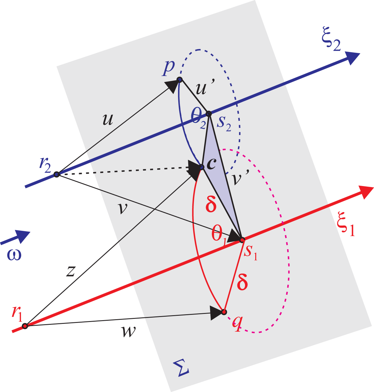
Geometry representation of the solution to generalized subproblem 2, parallel axes case.

The problem is now reduced to finding angle θ₂ to rotate the point p around the axis of the screw ξ₂ to come at the distance δ from the point s ₁, where

$s_1=r_1+\omega \cdot \left({\omega }^T\cdot \left(q-r_1\right)\right)$

37

That means to call subproblem 3 to find angle θ₂ and then to call subproblem 1 to find angle θ₁.

Obviously, all the points p, q, and s ₁ need to lie on the same plane normal to ω, so the first necessary condition for the solution existence is

${\omega }^T\cdot \left(p-s_1\right)=0$

38

In algorithmic manner, following two steps should be done if equation (38) is satisfied.

Step 1

Call the subproblem 3 with p, s ₁, ξ₂, and δ. Subproblem 3 solution details can be found in the study by Murray et al. ⁵

Let r ₂ be arbitrary point on the axis of the screw ξ₂. Geometrically, there is a solution if the circle centered at s ₂ (orthogonal projection of the point p on the axis of the screw ξ₂) with radius

$R=\Vert p-r_2-\omega \cdot {\omega }^T\cdot \left(p-r_2\right)\Vert$

39

intersects the circle centered at s ₁ with radius δ.

Because of equation (38), the condition

$\delta \ge \left|{\omega }^T\cdot \left(p-s_1\right)\right|$

40

is satisfied. Denote

$u=p-r_2,v=s_1-r_2$

41

$u\prime =u-\omega \cdot {\omega }^T\cdot u,v\prime =v-\omega \cdot {\omega }^{T}v$

42

Second necessary condition for solution existence is

$\left|{\Vert u\prime \Vert }^2+{\Vert v\prime \Vert }^2-{\delta }^2\right|\le 2\Vert u\prime \Vert \cdot \Vert v\prime \Vert$

43

Suppose u′ ≠ o and δ > 0. If the condition given in equation (43) is satisfied, then using the law of cosine follows

${\theta }_2=\text{atan2}\left({\omega }^T\cdot \left(u\prime \times v\prime \right),u{\prime }^T\cdot v\prime \right)\pm {\text{cos}}^{-1}\left(\frac{{\Vert u\prime \Vert }^2+{\Vert v\prime \Vert }^2-{\delta }^2}{2\Vert u\prime \Vert \cdot \Vert v\prime \Vert }\right)$

44

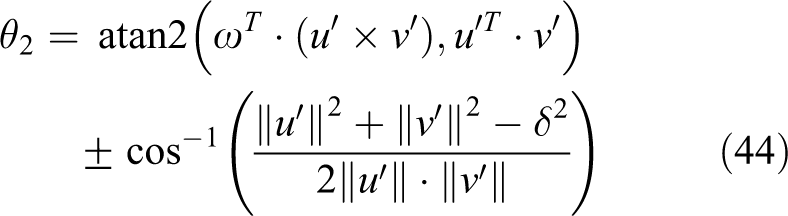
If inequality in equation (43) is strict, there are two angles θ₁₂ and θ₂₂ obtained from equation (44). If equality is hold in equation (43), then both of the circles touch each other, so there is unique angle θ₂.

Step 2

For every angle θ₂, obtained in step 1, call the subproblem 1, with q, ξ₁, and c, where

$c=e^{{\widehat{\xi }}_2{\theta }_2}p$

45

Denote

$z=c-r_1;w=q-r_1$

46

$z\prime =z-\omega \cdot {\omega }^T\cdot z,w\prime =w-\omega \cdot {\omega }^T\cdot w$

47

The angle θ₁ is then determined by

${\theta }_1=\text{atan2}\left({\omega }^T\left(z{\prime }^{\prime }\times w\prime \right),z{\prime }^T\cdot w\right)$

48

If u′ = o, then the point p lies on the axis of the screw ξ₂, so there is no solution in the case $\Vert p-s_1\Vert \ne \delta$ . If additionally, $\Vert p-s_1\Vert =\delta$ , there are infinitely many solutions—θ₂ could be any angle and θ₁ is determined by equation (48).

The case v′ = o is not possible, since it leads to conclusion s ₁ lies on the axis of the screw ξ₁, what is contrary to the assumption the axes of both of the screws are parallel.

If δ = 0, then q lies on the axis of the screw ξ₁ and q = s ₁. The problem is then reduced to subproblem 1 and if equation (38) is satisfied and $\Vert u\prime \Vert =\Vert v\prime \Vert \ne 0$ , then there is a unique solution for θ₂ obtained by equation (44) and θ₁ is any angle (infinitely many solutions); otherwise, there is no solution.

Extension of subproblem 2: New subproblem

In the previous section, a detailed elaboration about the generalization of Paden–Kahan subproblem 2 was given, and now this subproblem 2 can be used in general case without a consideration about the actual position of the axes of rotation. However, the given generalization of the subproblem 2 as well as the three Paden–Kahan subproblems are not enough to solve the inverse kinematics of a robot with general configuration. Chen et al. ²² noted that the solution for inverse kinematics of a serial robot with 6-DOF ‘Qianjiang I’ using the three well-known Paden–Kahan subproblems, as they are originally formulated, is impossible. So, they formulated a new subproblem just to solve the inverse kinematics of the above-mentioned robot.

The new subproblem comprises of a rotation of a point p (shown in Figure 3) about three axes of zero-pitch twists ξ₃, ξ₂, and ξ₁ successively, such that it coincides with a given point q. Thereto the axes of twists ξ₂ and ξ₃, respectively, are parallel to each other and the first axis, the axis of twist ξ₁ is not parallel to the remaining two axes and does not lie in the same plane neither with the axis of twist ξ₂ nor axis of twist ξ₃. In order to solve the new subproblem, the angles θ₁, θ₂, and θ₃ have to be determined, such that

$e^{{\widehat{\xi }}_1{\theta }_1}{e}^{{\widehat{\xi }}_2{\theta }_2}{e}^{{\widehat{\xi }}_3{\theta }_3}p=q$

49

Figure 3.

Geometry representation of the extended subproblem 2 solution.

So, the point p first rotates about the green axis of twist ξ₃ by angle θ₃, in Figure 3 represented by yellow arc, then it rotates about the blue axis of twists ξ₂ by angle θ₂ represented by the dark blue arc and at the end it rotates about the red axis of twists ξ₁ by angle θ₁ represented by the red arc.

Chen et al. ²² gave complete solution, but as a part of the solution, they used the assumption that the axis of twist ξ₁ is perpendicular to the two remaining axes of twists ξ₂ and ξ₃. Again, the solution of this new subproblem is not a general one.

In this article, a new geometric solution is given to this new subproblem in general case, where the axis of twist ξ₁ is in an arbitrary position and does not have to be perpendicular to the other axes of twists ξ₂ and ξ₃. This solution only excludes the position when the axis of twist ξ₁ is parallel to the other two axes, but this case does not have to be taken into account because the problem definition excluded this case. In this new geometric solution, the generalized Paden–Kahan subproblem 2 is used, with the case, when the two axes are parallel to each other that was detailed in the previous section.

Let ω₁ be the unit vector in a direction of the first axis of twist ξ₁ and ω₂ be the unit vectors in a direction of the two parallel axes of twists ξ₂ and ξ₃. Figure 3 visualizes the new geometrical solution that is constituted of four steps, explained below.

Step 1

Determine the plane ∑₁, the plane of the red circle that is normal to the unit vector ω₁ and passes through the point q. Determine the plane ∑₂, the plane of a green circle that is normal to the unit vector ω₂ and passes through the point p. Next, determine the line l(t) that is the intersection of these two planes ∑₁ and ∑₂ (Figure 3)

$l\left(t\right)=l_0+t\cdot d$

50

This intersecting line l(t) is determined, since the unit vectors ω₁ and ω₂ are not parallel to each other.

Step 2

Determine the projection s of the point q on the axis of the twist ξ₁

$s=s_1+{\omega }_1\left({\omega }_1^T\cdot \left(q-s_1\right)\right)$

51

where s ₁ is an arbitrary point on the axis of the twist ξ₁.

Step 3

Determine the intersection q_c between the line l(t) and a circle k ₁ centered in the point s with radius

$R=\Vert q-s\Vert$

52

on the plane ∑₁.

To find the intersection of the line l(t) and a circle, one needs to find the roots of a quadratic equation with t as an unknown. From the value of the discriminant D of the quadratic equation depends whether the line l(t) intersects the circle or not, and if it does, in how many points

$D={\left(2l_0^T\cdot d-2d^T\cdot s\right)}^2-4\left({\Vert l_0\Vert }^2-2l_0^T\cdot s-{\Vert q\Vert }^2+2q^T\cdot s\right)$

53

Step 4

If D < 0, then the line l(t) doesn’t intersect the circle k ₁, and the new subproblem does not have a solution.

If D = 0 then the line l(t) and the circle k ₁ have one common point q_c

$q_c=l_0+td$

54

where $t=l_0^T\cdot d-d^T\cdot s$ .

Once the point q_c is determined, the angle θ₁ can be found by calling the Paden–Kahan subproblem 1, so that the point q_c coincides with the point q when it rotates about the axis of twist ξ₁

$e^{{\widehat{\xi }}_1{\theta }_1}{q}_c=q$

55

The two remaining unknown angles θ₂ and θ₃ can be determined by calling the Paden–Kahan subproblem 2, so that the point p first rotates about the axis of twist ξ₃ and then rotates about the axis with twist ξ₂ to coincides with point q_c

$e^{{\widehat{\xi }}_2{\theta }_2}{e}^{{\widehat{\xi }}_3{\theta }_3}p=q_c$

56

Here, the original formulation of Padern–Kahan subproblem 2 is not used, but our generalized version of this subproblem 2 detailed in the previous section, because the axes of twists ξ₂ and ξ₃ are parallel to each other, and case 2b needs to be considered.

If D > 0 then the line l(t) intersect the circle k ₁ in two points q_{c 1} and q_{c 2} that can be determined

$q_{c1}=l_0+t_{1}d\hspace{0.17em}\text{and}\hspace{0.17em}{q}_{c2}=l_0+t_{2}d$

57

where $t_{1/2}=\frac{-\left(2l_0^T\cdot d-d^T\cdot s\right)\pm \sqrt{D}}{2}$

In this case in order to determine the unknown angles θ₁, θ₂, and θ₃, again it has to be done by calling of the Paden–Kahan subproblems 1 and 2 in the same manner like in the previously detailed case when D = 0, but two times: once for the point q_{c 1} and then the same for the point q_{c 2}. At the end, the solution is a set of two or four triples of angles, if the given data satisfy necessary conditions for existence and uniqueness of the solution in generalized subproblem 2.

Examples, experiments and results

Kinematic model of 6-DOF industrial robot

We have used kinematic model based on the screw theory and our geometric algorithms as a part of experiment for accuracy improvement of 6-DOF industrial robot KUKA KR 360 R2830, manufactured by KUKA AG company.

Using the scheme shown in Figure 4 and the notations explained in “Introduction” section, construction of the twists for pure rotation are made according to equation (7)

$\begin{array}{l}{\omega }_1=\left[\begin{array}{c}0\\ 0\\ 1\end{array}\right]\hspace{0.17em}{\omega }_2=\left[\begin{array}{c}0\\ -1\\ 0\end{array}\right]\hspace{0.17em}{\omega }_3=\left[\begin{array}{c}0\\ -1\\ 0\end{array}\right]\\ {\omega }_4=\left[\begin{array}{c}-1\\ 0\\ 0\end{array}\right]\hspace{0.17em}{\omega }_5=\left[\begin{array}{c}0\\ -1\\ 0\end{array}\right]\hspace{0.17em}{\omega }_6=\left[\begin{array}{c}-1\\ 0\\ 0\end{array}\right]\\ q_1=\left[\begin{array}{c}0\\ 0\\ 0\end{array}\right]\hspace{0.17em}{q}_2=\left[\begin{array}{c}{a}_1\\ 0\\ d_1\end{array}\right]\hspace{0.17em}{q}_3=\left[\begin{array}{c}{a}_{{\hspace{0.17em}}_1}\\ 0\\ d_{{\hspace{0.17em}}_1}+d_2\end{array}\right]\\ q_4=q_5=q_6=\left[\begin{array}{c}{a}_1+a_3\\ 0\\ d_1+d_2+d_3\end{array}\right]\\ {\xi }_1=\left[\begin{array}{c}0\\ 0\\ 0\\ 0\\ 0\\ 1\end{array}\right]\hspace{0.17em}{\xi }_2=\left[\begin{array}{c}{d}_1\\ 0\\ a_1\\ 0\\ -1\\ 0\end{array}\right]\hspace{0.17em}{\xi }_3=\left[\begin{array}{c}{d}_1+d_2\\ 0\\ a_1\\ 0\\ -1\\ 0\end{array}\right]\\ {\xi }_4={\xi }_6=\left[\begin{array}{c}0\\ -d_1-d_2-d_3\\ 0\\ -1\\ 0\\ 0\end{array}\right]\hspace{0.17em}{\xi }_5=\left[\begin{array}{c}{d}_1+d_2+d_3\\ 0\\ -\left(a_1+a_3\right)\\ 0\\ -1\\ 0\end{array}\right]\end{array}$

58

Figure 4.

Coordinate frames scheme.

Initial configuration is the transformation matrix of the robot’s tool with respect to the robot base, when all of the joint angles are zeros. It is determined by

$g_{bt}\left(0\right)=\left[\begin{array}{cccc}1& 0& 0& a_1+a_3+a_6\\ 0& 1& 0& 0\\ 0& 0& 1& d_1+d_2+d_3\\ 0& 0& 0& 1\end{array}\right]$

59

According to equation (12), the forward kinematics is determined by the matrix

$g_{bt}\left(\theta \right)=e^{{\widehat{\xi }}_1{\theta }_1}{e}^{{\widehat{\xi }}_2{\theta }_2}{e}^{{\widehat{\xi }}_3{\theta }_3}{e}^{{\widehat{\xi }}_4{\theta }_4}{e}^{{\widehat{\xi }}_5{\theta }_5}{e}^{{\widehat{\xi }}_6{\theta }_6}{g}_{bt}\left(0\right)$

60

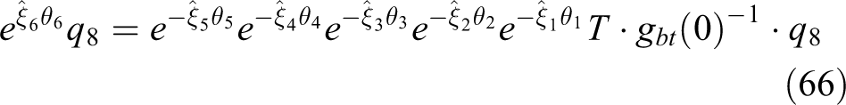
Inverse kinematics solution: If a pose is given, as position and orientation with matrix T, the vector θ of machine coordinates should be found

$T=\left[\begin{array}{cccc}{n}_x& o_x& l_x& p_x\\ n_y& o_y& l_y& p_y\\ n_z& o_z& l_z& p_z\\ 0& 0& 0& 1\end{array}\right]$

61

Since the point q ₆ lies on all three last axes, from equation (60) and the equation $g_{bt}\left(\theta \right)=T$ follows

$e^{{\widehat{\xi }}_1{\theta }_1}{e}^{{\widehat{\xi }}_2{\theta }_2}{e}^{{\widehat{\xi }}_3{\theta }_3}{q}_6=T\cdot g_{bt}{\left(0\right)}^{-1}\cdot q_6$

62

Finding θ₁, θ₂, and θ₃ is now reduced to applying the extended subproblem 2—the new subproblem explained in the previous section, since axes of the twists ξ₂ and ξ₃ are parallel, and the axis of the twist ξ₁ is not parallel to the remaining two axes and does not lie in the same plane neither with the axis of twist ξ₂ nor axis of twist ξ₃.

Taking into consideration, the obtained values for θ₁, θ₂, and θ₃ and that the point

$q_7=\left[\begin{array}{c}{a}_1+a_3+a_6\\ 0\\ d_1+d_2+d_3\end{array}\right]$

63

lies on the axis of the twist ξ₆, applying the standard Paden–Kahan subproblem 2 yields the solution for θ₄ and θ₅, since

$e^{{\widehat{\xi }}_4{\theta }_4}{e}^{{\widehat{\xi }}_5{\theta }_5}{q}_7=e^{-{\widehat{\xi }}_3{\theta }_3}{e}^{-{\widehat{\xi }}_2{\theta }_2}{e}^{-{\widehat{\xi }}_1{\theta }_1}T\cdot g_{bt}{\left(0\right)}^{-1}\cdot q_7$

64

Finally, any referent point on the axis of the twist ξ₅, different from q ₆ can be used for obtaining the angle θ₆, applying the standard Paden–Kahan subproblem 1. For instance, taking the point

$q_8=q_6+\left[\begin{array}{c}0\\ b\\ 0\end{array}\right]=\left[\begin{array}{c}{a}_1+a_3\\ b\\ d_1+d_2+d_3\end{array}\right]$

65

and using the equation

$e^{{\widehat{\xi }}_6{\theta }_6}{q}_8=e^{-{\widehat{\xi }}_5{\theta }_5}{e}^{-{\widehat{\xi }}_4{\theta }_4}{e}^{-{\widehat{\xi }}_3{\theta }_3}{e}^{-{\widehat{\xi }}_2{\theta }_2}{e}^{-{\widehat{\xi }}_1{\theta }_1}T\cdot g_{bt}{\left(0\right)}^{-1}\cdot q_8$

66

the last angle θ₆ is obtained.

The validity of the algorithm is confirmed by taking the parameters values

$\begin{array}{l}{a}_1=500;\hspace{0.17em}{a}_3=1025;\hspace{0.17em}{a}_6=290;\hspace{0.17em}b=200\\ d_1=1045;\hspace{0.17em}{d}_2=1300;\hspace{0.17em}{d}_3=-55\end{array}$

$d_1=1045;\hspace{0.17em}{d}_2=1300;\hspace{0.17em}{d}_3=-55$

67

and pose matrix

$T=\left[\begin{array}{cccc}0.11699& -0.83031& -0.54489& 628.93\\ 0.90972& 0.30968& -0.27659& 1294.40\\ 0.39839& -0.46335& 0.79158& 2414.96\\ 0& 0& 0& 1\end{array}\right]$

68

obtained applying forward kinematics algorithm, taking machine coordinates

$\theta =\left[\frac{\pi }{3},\frac{\pi }{12},-\frac{\pi }{15},\frac{\pi }{4},\frac{\pi }{6},-\frac{\pi }{9}\right]$

69

Proposed inverse kinematics procedure is applied and eight solutions are obtained, shown in Table 1. All these solutions are checked by simulation and forward kinematics procedure and all of them lead to desired pose (68) with maximal orientation deviation of 3.5 × 10⁻¹⁵ and maximal position deviation of 1.5 × 10⁻¹² mm.

Table 1.

Eight solutions of inverse kinematics.

Solution #	Joint #	θ (°)	Solution #	Joint #	θ (°)
1	1	60.0000	2	1	60.0000
	2	15.0000		2	15.0000
	3	−12.0000		3	−12.0000
	4	45.0000		4	−135.0000
	5	30.0000		5	−30.0000
	6	−20.0000		6	160.0000
3	1	60.0000	4	1	60.0000
	2	−72.6269		2	−72.6269
	3	−161.8571		3	−161.8571
	4	158.9850		4	−21.0150
	5	99.6360		5	−99.6360
	6	−162.7859		6	17.2141
5	1	−120.0000	6	1	−120.0000
	2	31.2018		2	31.2018
	3	−216.1085		3	−216.1085
	4	−132.5502		4	47.4498
	5	28.6805		5	−28.6805
	6	−22.8099		6	157.1901
7	1	−120.0000	8	1	−120.0000
	2	75.6283		2	75.6283
	3	42.2514		3	42.2514
	4	−32.1828		4	147.8172
	5	41.5901		5	−41.5901
	6	−133.9015		6	46.0985

Algorithm testing on 7-DOF AFP machine

The geometric algorithm presented in the previous section was implemented in the postprocessor part of MikroPlace [version 4.0]—software for off-line programming, design and simulation of automated fiber placement (AFP) and automatic tape layup (ATL) machines. Specifically, it was experimentally tested on AFP machine with 7 DOF—three linear axes and four rotational, deployed in the next parent/child order:

Linear X → Linear Y → Linear Z → Rotation Z → Rotation X → Rotation Z and another free axis Rotation around X (Figure 5).

Figure 5.

7-DOF AFP Machine. DOF: degrees of freedom; AFP: automated fiber placement.

The algorithm was tested on different mandrel shapes covering the two general types of mandrel geometry:

Open shape surface mandrel (flat, shaped parabolic) (Figure 6(a)) and

Closed surfaces—360° rotational mandrel surfaces (Figure 6(b)).

Figure 6.

Open (a) and closed (b) surface mandrel.

The layup was under different layup angles in order to test more axes combination. Figure 7 shows different machine positions on the software simulation.

Figure 7.

AFP Machine simulation. AFP: automated fiber placement.

In Figure 8, the actual laid material is shown.

Figure 8.

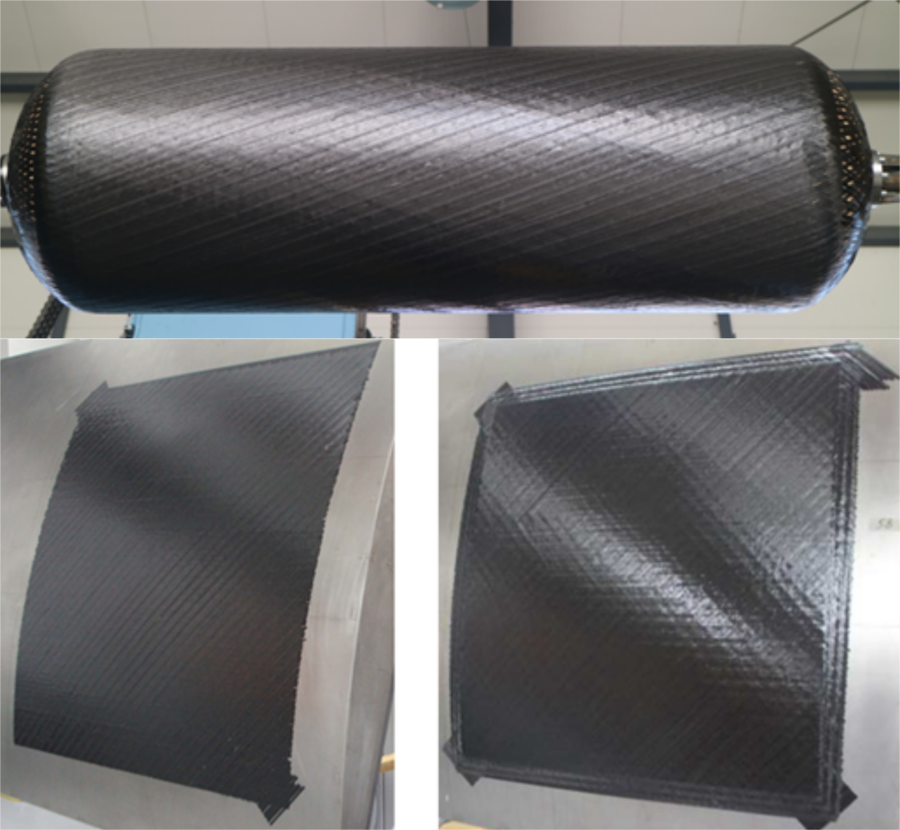
AFP technology product. AFP: automated fiber placement.

Conclusion

Concentrating on the necessary and sufficient conditions, as well as the number of solutions for the inverse kinematics of the robot manipulator in order to transfer from pose to machine space coordinates, this article has presented a geometric algorithm that can be applied on multiple movement configurations. Three basic Paden–Kahan subproblems of screw theory were used in order to extend subproblem 2 designed not to depend on the mutual positioning of the screw axes. The article sets and solves (giving an algorithmic approach) a new subproblem where three independent screw axes are used in order to move the manipulator from one to another point in the space. Practically, this subproblem is used to solve a specific configuration of a 6-DOF robot that cannot be solved using the three well-known Paden–Kahan subproblems. The algorithms given here, solve the problem of inverse kinematics generally, so when they are implemented in some programming language there is no need to look after the mutual positioning of the axes of rotation. Finally, combining the algorithms presented in this article gives a wider use of the screw theory based methods for several differently configured manipulators.

Although, this article has been specifically focused on the step-by-step geometric algorithm for the solution of extended Paden–Kahan subproblems, these are the key algorithms to the actual inverse kinematics implementation for robotic movement and industrial gantry type machines with multiple movement axes.