Analysis of control and correction options of mobile robot trajectory by an inertial navigation system

Abstract

The article deals with the research of the supplementation of industrial robot effector trajectory’s control systems by an inertial navigation system. The method of reverse validation and location of an object in a navigated reference system does not require additional calibration. The goal of the research is to verify the assumption that it is possible to control and correct the programmed mobile robot trajectory by implementing an inertial navigation system even in a case when the inertial navigation system is used as the only trajectory control device. The data obtained are processed by the proposed and detailed application.

Introduction

The first and still significant area of robot research and development was their deployment in an industry. At the beginning, industrial robots performed simple manipulations of parts and materials or finished products. By gradually improving their management, their application has been extended to the area of direct production. The challenges that emerged from their roles have also revolutionized the control of robotic equipment management. The development and deployment of various sensors required considerable investments. Nowadays, when these systems are developed at a high technological level, there remains the possibility of looking for other, more affordable, tracking, and correction solutions for the trajectory.

The industrial robot, often referred to as the “working head,” is a power member of the robotic device—it performs the tasks defined by the production process. Knowing the course of his trajectory at the given performance is a wanted value. The construction and mechanical limitations of the industrial robot induce deviations into the desired effector movement along the programmed trajectory. The resulting errors must be measured and evaluated, resulting in the modification of the effector trajectory so that the industrial robot can perform its tasks with an acceptable accuracy. Different measurement sensors (visual, contact, and other sensors) are used to measure the inaccuracy of the trajectory. The disadvantages of their deployment include high initial costs and frequent calibration of the control system.

We investigate the possibility of replacing the control devices of an industrial robot effector trajectory with an inertial navigation system (INS) device that does not require additional calibration due to the method of the location of the object in the navigation reference system.

The possibilities of using INS in robotics and industrial robotics have been addressed by several authors. Lai et al. analyzed the INS vibrational errors in unmanned aerial vehicles ¹ ; Wang et al. described the possibilities of inertial navigation for small unmanned aircrafts ² ; Qazizada and Pivarčiová described the possibilities of their application for inertial navigation of the mobile robot ³ ; Turygin et al. described the possibilities of increasing the reliability of the mobile robot control process through reverse validation. ⁴ Lobo et al. described a prototype of an INS for use in mobile land vehicles, such as cars or mobile robots. ⁵ Nemec et al. used inertial sensors for control of the mobile robot by hand movement. ⁶ Božek and Šuriansky described inertial system-based robot control. ⁷ Pirník et al. studied the integration of inertial sensor data into control of the mobile platform. ⁸

Our goal is to design an application that checks and makes the necessary adjustments to the robot trajectory. We study the validity of the assumption whether it is possible to control and correct the programmed robot trajectory by implementing an INS. Even in the proposed case, the INS is used as the sole trajectory control device and its data are suitably processed by the proposed application. Using the AL5B robot model with an angular motion and hardware, we created an industrial robot simulation. The INS x-inertial measuring unit (IMU) was placed at the end point of the robot’s effector (EE point).

We explored the possibility of real-time processing of IMU data, so we developed an application with a modified integrated component filter for calculated values of speed and position. In addition, we also dealt with a different way to gather information about moving of the device (when the object is moving or not moving). For the proposed application, we used an optimized Madgwick Attitude and Heading Reference Systems (AHRS) algorithm, based on a gradient of descent optimization (vertical movement), its parameter used to control the convergence rate (indicative estimate with the optimum weight of the contribution from each sensor).

Kinematics of industrial robots

The kinematics of industrial robots generally determine the position of the EE point in the space based on the parameters of the rotation (or extension) of the individual joints and arms. For the angular type of motion, three rotary axes are characteristic, with the robot having six degrees-of-freedom. The first step in calculating the forward kinematics is to identify translational and rotational movements. When applying the Denavit–Hartenberg convention, we choose the orientation where the axis is directed vertically. This orientation rule is advantageous for the calculation because three of the four movements are performed around the x-axis. When identifying, it is necessary to proceed from the EE point toward the robot base. We also repeat the procedure when calculating the resulting transformation matrix. ⁹ In addition to the first angular robot kinematics, all other members perform rotary movements in the selected coordinate system around the x-axis, the change of position being dependent, in addition to the rotational angle, also from the distance of the rotation axis from the EE point. By applying these considerations, it is possible to compile the identified data in Table 1.

Table 1.

Parameters of Denavit–Hartenberg convention for robot model AL5B.

i	αi –1	ai –1	di	Θi
1	0	0	d 1	Θ 1
2	90	0	0	Θ 2
3	0	a 3	0	Θ 3
4	0	a 4	0	Θ 4–90

The individual homogeneous transformation matrices (1) are arranged so that the first identified homogeneous transformation matrix $T_4^3$ is the right and the last $T_1^0$ to the left (C _i —cosine Θ_i , S _i —sine). The final transformation matrix (2) has the designation $T_4^0$ , where the first three columns represent the orientation of the EE point and the last column represents its position (at the constant scale of the scale 1). To calculate forward kinematics, the input parameters are specific values of the goniometric functions of the respective rotational angles. Subsequently, a multiplication of four matrices is performed to obtain the resulting transformation matrix. ⁹ Managing inverse kinematics is a more complex task because of the absence of a universal solution—the system of calculation is dependent on the structure and limitations of the movements of an angular industrial robot. The input parameters—the coordinates of the EE point in the Cartesian system x, z, and y—are specified in the calculation. The task is to find the values of all rotating angles in the system. There are several methods based on differential geometry when almost all of them use auxiliary position vectors connecting individual members of the system to calculate the angles held by parts of the robot. The complication is to find the correct layout and orientation of the calculated parameters so that the solution is feasible to execute

$\begin{array}{l}{T}_1^0=\left[\begin{array}{cccc}{\text{C}}_{{\theta }_1}& -{\text{S}}_{{\theta }_1}& 0& 0\\ {\text{S}}_{{\theta }_1}& {\text{C}}_{{\theta }_1}& 0& 0\\ 0& 1& 0& d_1\\ 0& 0& 0& 1\end{array}\right] T_2^1=\left[\begin{array}{cccc}{\text{C}}_{{\theta }_2}& -{\text{S}}_{{\theta }_2}& 0& 0\\ 0& 0& -1& 0\\ {\text{S}}_{{\theta }_2}& {\text{C}}_{{\theta }_2}& 0& 0\\ 0& 0& 0& 1\end{array}\right]\\ T_3^2=\left[\begin{array}{cccc}{\text{C}}_{{\theta }_3}& -{\text{S}}_{{\theta }_3}& 0& a_3\\ {\text{S}}_{{\theta }_3}& {\text{C}}_{{\theta }_3}& 0& 0\\ 0& 0& 1& 0\\ 0& 0& 0& 1\end{array}\right] T_4^3=\left[\begin{array}{cccc}{\text{C}}_{{\theta }_4}& -{\text{S}}_{{\theta }_4}& 0& a_4\\ {\text{S}}_{{\theta }_4}& {\text{C}}_{{\theta }_4}& 0& 0\\ 0& 0& 1& 0\\ 0& 0& 0& 1\end{array}\right]\end{array}$

1

$T_4^0=T_1^0{T}_2^1{T}_3^2{T}_4^3=\left[\begin{array}{cccc}{n}_x& o_x& a_x& d_x\\ n_y& o_y& a_y& d_y\\ n_z& o_z& a_z& d_z\\ 0& 0& 0& 1\end{array}\right]$

2

Filtering and processing of IMU sensor signals

Signal errors originating from INS sensors can be divided according to the cause of their occurrences to internal ones (caused by sensor manufacturing technology) and errors caused by external influences (ambient temperature and pressure, sudden changes in the magnetic field of the earth, etc.). To obtain the desired values (position, orientation, and speed), the signal is further filtered and integrated according to the time, which is the gradual increase in the value of the measured value deviation in time. Therefore, it is necessary to identify the impacts, to understand the cause of their occurrence, to estimate their future course, and subsequently to modify the values of the sought-after quantities.

If we did not remove the deviations in the acceleration measurements, they would be present in the double integration, which ultimately causes them to increase—the constant acceleration error (accelerometer) will manifest itself as the linear velocity and the quadratic magnitude of the error in the position. Similarly, a constant error of the angular velocity (gyroscope) is shown as the quadratic velocity error rate and the cubic error size in the position.

Although the IMU remains in peace, it constantly measures the forces that are the result of the inertial frame measurement—it is firmly connected in space and time, the center of gravity is in the middle of the earth, and the nonrotating axes are with respect to the position of the stars (the Z_i axis is parallel to the earth’s axis of rotation, the X_i axis points to the spring point, and the Y_i axis is perpendicular to both axes—completes the system as right-handed and rectangular). Similarly, the gravitational acceleration of the earth (about 9.8 m/s²) is measured continuously by the accelerometer and partly influences the gyroscopes. ¹⁰

The input signal range is the maximum acceleration value or angular rate that can be recorded by the IMU sensors of the device. Out-of-range values lead to erroneous measurements, so the data are important when choosing a filtering method. Another error that needs to be identified is the measured value deviation (bias), which is evaluated when the IMU is turned on and during inrun bias. Scale factor is the difference between the input and the output of the metering unit. To minimize the continuous signal noise (random walk or sensor noise), which has a stochastic character, statistical methods and mathematical models are used. The noise itself is present in the signal even after applying the statistical deviation, but its size is significantly reduced to an acceptable rate. ¹¹

After processing the signal using the Kalman filter (code class by x-IMU producer), we obtain a more accurate specification of its noise and, at the same time, smoother performance.

Calculation of velocity and INS location in reference system

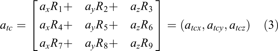
The calculation of speed and position is carried out by a series of IMU sensor signal processing. After obtaining the measured values from the sensors (accelerometer, gyroscope, and magnetometer), we use the AHRS algorithm whose product is also the rotary matrix R. The data from the matrix will be used to compensate the acceleration of the accelerometer (3) in the reference system relative to the direction of the earth’s attraction

$a_{tc}=\left[\begin{array}{ccc}{a}_x{R}_1+& a_y{R}_2+& a_z{R}_3\\ a_x{R}_4+& a_y{R}_5+& a_z{R}_6\\ a_x{R}_7+& a_y{R}_8+& a_z{R}_9\end{array}\right]=(a_{tcx},a_{tcy},a_{tcz})$

3

Before the second adjustment, it is important to recalculate gravitational acceleration due to the IMU tilt around the axis of the navigated coordinate system. Gravitational acceleration is the magnitude attributed to the object by gravitational force and expresses the intensity of the gravitational field. The accelerometer system captures the individual components of the acceleration vector g = (g_{x ,} g_{y ,} g_z ) with the gravitational acceleration relation g ² = g ² _x + g ² _y + g ² _z . Using Pythagoras, we can calculate the magnitudes of the individual components of gravitational acceleration (4) if we include the known values of Euler angles in the calculation. The angle φ represents the rotation around the x-axis and the angle θ is rotated about the y-axis. We will not use the angle α of the rotation around the z-axis until the calculation (earth’s attraction is perpendicular to the plane in which it lies)

$g_x=-g\cdot \text{sin}\theta g_y=g\cdot \text{cos}\theta \cdot \text{sin}\phi g_z=g\cdot \text{cos}\theta \cdot \text{cos}\phi$

4

Second, the linear acceleration (5) is calculated in the earth-centered earth-fixed frame, which removes the calculated gravitational values in the individual acceleration components

$a_{\text{lin}}=\left[\begin{array}{c}{a}_{tcx}\cdot g_x\\ a_{tcy}\cdot g_y\\ (a_{tcz}-1)\cdot g_z\end{array}\right]=(a_{\text{lin}x},a_{\text{lin}y},a_{\text{lin}z})$

5

After numerical editing, we received the linear acceleration values in all three axes x, y, and z. The first integration follows by time (in our case, the value of the period Δt is 1/256 = 0.00390625 s). The instantaneous matrix function (6) is iterative—the previous value of the calculated velocity of the u _lin is added to the new value of linear acceleration (which we integrate). The resulting values serve as input parameters for the first-order Butterworth high-pass filter (each component of the speed is separately filtered). The filter’s product is a matrix of instantaneous object velocities in the x, y, and z directions cleared of undesirable integration errors

$v_{\text{lin}}=\underset{t_1}{\overset{t_2}{{\displaystyle \int }}}{a}_{\text{lin}}\text{d}t=u_{\text{lin}}+a_{\text{lin}}\cdot \Delta t=\left[\begin{array}{c}{u}_{\text{lin}x}+a_{\text{lin}x}\cdot \Delta t\\ u_{\text{lin}y}+a_{\text{lin}y}\cdot \Delta t\\ u_{\text{lin}z}+a_{\text{lin}z}\cdot \Delta t\end{array}\right]=\left(v_{\text{lin}x},v_{\text{lin}y},v_{\text{lin}z}\right)$

6

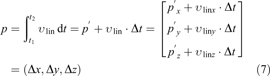
In the third step, the velocity values are integrated, obtaining the matrix function of the position (7), which is also iterative—the previous value of the calculated position p′ is added to the new instantaneous speed data. The calculated values are refiltered using the first-order Butterworth high-pass filter. The resulting filter product is a matrix of coordinate objects in the navigated coordinate system

$p={\displaystyle {\int }_{t_1}^{t_2}{\upsilon }_{\text{lin}}\text{d}t=p^{\prime }+{\upsilon }_{\text{lin}}\cdot \Delta t=\left[\begin{array}{c}{p^{\prime }}_x+{\upsilon }_{\text{lin}x}\cdot \Delta t\\ {p^{\prime }}_y+{\upsilon }_{\text{lin}y}\cdot \Delta t\\ {p^{\prime }}_z+{\upsilon }_{\text{lin}z}\cdot \Delta t\end{array}\right]}=(\Delta x,\Delta y,\Delta z)$

7

Used hardware

The location data of the EE point of the robot model in the space were obtained by attaching the x-IMU to the robot construction and positioning near the given point. The device uses the AHRS algorithm. Platforms include sensors, the processor to calculate measured values and eight UART ports (analog I/O interface), and USB and Bluetooth interface. There is also a custom application interface. The sensor system consists of a triaxial 16-bit gyroscope (range: ± 2000°/s), a triaxial 12-bit accelerometer (range: ± 8 g), a triaxial 12-bit magnetometer (range: ± 8.1 G), and a 16-bit thermometer. The device is calibrated directly by the manufacturer. ¹²

Model of the AL5B robot from company Lynxmotion performs an angular motion with four degrees-of-freedom. The design model consists of individual parts with the possibility of modifying them. The kit includes mechanical parts—servomotors and construction parts: base, shoulder, elbow, and wrist. Various available effectors are attached to the wrist (the used device has a mounted drive with a rotary drive). Servomotors are powered by a 5 V (3 A) power supply. Servomotors are manufactured by Hitec. All servomotors have their own limitations of rotation ranges from 0° to 180°, while the rotation range of the last servomotor is rotated by 90°. ¹³

Micro Maestro 6-Channel USB Servo Controller provides an integrated controller for controlling six servomotors. The advantage of the device is the ability to control servomotors through programming scripts in a custom API. The power supply is via the USB interface (5–16 V), the pulse width is from 0.064 ms to 3.28 ms, and the repetition frequency is in the range from 33 Hz to 100 Hz. ¹⁴

Design of application for control and trajectory correction of the industrial robot

The diagram (Figure 1) shows the connection of individual devices and their mutual communication links. It represents a simulation of the industrial robot model (we used the robot model AL5B). The proposed application is installed on the control computer. The programmed trajectory is stored in the comma-separated values file. Trajectory instructions are loaded into the application and executed by the user interface.

Figure 1.

Scheme of used devices and connections between them.

Block scheme of designed application

The application program is divided into three logical units. In the block diagram (Figure 2), they are displayed at the top of the program. The data stream is displayed with oriented full lines (the arrow shows the data flow direction). The communication between the logic of the program as well as the communication between the program and the application interfaces, libraries, and devices is shown by oriented dashed lines (arrows pointing to the direction of communication). The program uses the OSC_DLL external library with the appropriate oscilloscope generating module to graphically present the progress of the x-IMU device signals and communicates with the servo controller using the USC API application interface, enhanced by the USB wrapper library, to detect the device. It uses the x-IMU API application interface to communicate with the IMU. In addition to external libraries and APIs, the program implements filter classes for processing data from the x-IMU device. The first class is the Kalman filter, followed by the Madgwick AHRS algorithm. The last used class is the Butterworth high-pass filter.

Figure 2.

Block scheme of the designed application.

Design of program solution

When designing the program, we were inspired by the work of Sebastian O.H. Madgwick, presented during the Boston University PhD study (part of the work was published in November 2013 under Open Source license) under the title “Oscillatory Motion Tracking With x-IMU.” In this, it looked at mapping the x-IMU motion of the device in the Cartesian coordinate system, using dual integration, and then filtering the integrated values to obtain spatial coordinates. Acceleration data and angular velocity were first collected (from the entire course of the test motion) and further presented in graphical form (MATLAB). The test trajectory of the device was oscillating, attempting to eliminate the incrementally increasing error of measurement of the data, due to time integration (when the movement changes, zeroing of the acceleration values occurs). The Butterworth high-pass filter, which has high performance when all the measured data are collected, is used as the filtering algorithm of the integration components of the calculation, because backfill is run through a whole range of data and can result in the removal of most undesirable errors from the resultant results. ¹⁵

In our case, we explored the possibility of applying the described method of processing data from the IMU device in real time. Therefore, we designed a modified integration component filter for calculated speed and position. In addition, we dealt with a different way to get information about moving the device (when the object is moving or not moving).

Forward kinematics

If we want to control the movement of the robot model so that the EE point moves over the programmed trajectory, we need to know the coordinates of that point in the navigated coordinate system. In the case of forward kinematics, we have at the beginning of calculating the given rotational angles θ ₀–θ ₄ in the individual joints of the robot model (Figure 3). For the calculation, the knowledge of the size of the lengths of the individual segments (for identifying the translational movements of the robot) is required: d ₁—base distance from the x ₀-axis of the first joint; a ₂—the zero point of the x ₁-axis of the second joint (point A) from the null point of the x ₃ of the third joint (point B); a ₃—the distance of x ₂ and x ₃ axes between points B and C; a ₄—the zero-point distance x ₃ (point C) and EE point (point D).

Figure 3.

Variables used in the forward and inverse kinematics algorithm.

The algorithm consists of operations using goniometric functions and operations with vectors. The working geometric plane P (Figure 3) passes through the longitudinal axis of the robot construction and its parts. The product of the algorithm is the calculation of the vector $\overrightarrow{AD}$ and its coordinates in the plane P. Coordinates of the vector are determined from Pythagoras sentence $x_2=a_2\cdot \text{cos}{{\theta }^{\prime }}_1$ and $z_2=a_2\cdot \text{sin}{{\theta }^{\prime }}_1$ , while ${{\theta }^{\prime }}_1= {\theta }_1\iff {\theta }_1<90$ and ${{\theta }^{\prime }}_1= 180-{\theta }_1\iff {\theta }_1\ge 90$ . The second operation is to calculate the angle θ″₂ at point B, joining the “shoulder” portion and the horizontal line lying in the plane P and passing point B: ${{\theta }^{″}}_2= {\theta }_1-\left(180-{\theta }_2\right)$ . Coordinates x₃ and z₃ of the vector $\overrightarrow{BC}$ are counted similarly to the previous operation. The last operation of the algorithm is to calculate the angle θ″₃ at the point C, which is part of the “elbow” and the horizontal line passing through the point C: ${{\theta }^{″}}_3= {{\theta }^{″}}_2-\left(90-{\theta }_3\right)$ . Coordinates x₄ and z₄ of the vector $\overrightarrow{CD}$ are counted similarly to the first operation. The last operation of the algorithm is to calculate the coordinates for the vector $\overrightarrow{AD}$ in the working plane P: ${\overrightarrow{AD}}_y=\sqrt{a_2\cdot x_2+a_3\cdot x_3+a_4\cdot x_4}$ and ${\overrightarrow{AD}}_y=\sqrt{a_2\cdot y_2+a_3\cdot y_3+a_4\cdot y_4}$ . Using the first rotation angle θ ₀ and x-coordinate of the vector, we determine the orientation of the robot in the workspace (Figure 4)—parameter K (the value represents the position of the EE point in the corresponding quadrant of the plane of the ground).

Figure 4.

Orientation of the robot in the workspace and calculation of EE point coordinates.

The size of the auxiliary rotational angle θ′ ₀ ( $K=\text{I }\vee \text{III }\Rightarrow {{\theta }^{\prime }}_0={\theta }_0-90$ and $K=\text{II }\vee \text{IV }\Rightarrow {{\theta }^{\prime }}_0=90-{\theta }_0$ ) lying in the plane of the ground plane of the workspace can be deduced based on the K-value detected. The robot model has a limitation of rotation—it can rotate about the axis from only in the interval <0; 180>°. By finite operations for forward kinematics, we obtain the coordinates x, y, and z for the EE point in the navigated coordinate system:

$x=\sqrt{{\overrightarrow{AD}}_x\cdot \text{cos}{{\theta }^{\prime }}_0}$ when $=I\vee IV\Rightarrow x=-x$ ; $y=\sqrt{{\overrightarrow{AD}}_x\cdot \text{sin}{{\theta }^{\prime }}_0}$ when $K=III\vee IV\Rightarrow y=-y$ ; $z=d_1+{\overrightarrow{AD}}_y$ .

Inverse kinematics

We are looking for rotation angles of θ ₀–θ ₄. The initial condition for the calculation is that the input coordinates of the EE point are within the range of the robot model. The maximum distance we can reach from point A is the sum of the lengths of all parts of the robot maxL = a ₂ + a ₃ + a ₄. The length of the vector is $\left|\overrightarrow{AD}\right|=\sqrt{x^2+y^2+{\left(z-d_1\right)}^2}$ . If the expression $\left|\overrightarrow{AD}\right|>\text{max}L$  applies, the inverse kinematics algorithm stops and an error message is displayed. In the first step, we get the values of the rotation angle ${\theta }_0=t{g}^{-1}\left(\frac{x}{y}\right)$ (rotation around the axis from the robot model). Since we have to limit the rotation interval, we add the angle conversion factor: $({\theta }_0<0)\Rightarrow {\theta }_0=180+{\theta }_0$ . The next step is to determine the coordinate points $A\left[0;d_1\right]$ , $D\left[D_x;z\right]$ where $D_x=\sqrt{x^2+y^2}; \left(x<0\right)\Rightarrow D_x=-D_x$ and $A^{\prime }\left[0;2\cdot \left(D_z-d_1\right)+d_1\right]$ (auxiliary point) lying in the working geometric plane P. There is vector between points A and D, where we calculate the angle $\Omega ={\text{cos}}^{-1}\left(\frac{D_x-A_x}{\sqrt{{\left(D_x-A_x\right)}^2+{\left(D_z-A_z\right)}^2}}\right)$ which is formed by a unit vector $\overrightarrow{\left[0;0\right]\left[1;0\right]}$ on the x-axis, respectively, and the angle ${\Omega }^{\prime }={\text{cos}}^{-1}\left(\frac{D_x-{A^{\prime }}_x}{\sqrt{{\left(D_x-{A^{\prime }}_x\right)}^2+{\left(D_z-{A^{\prime }}_z\right)}^2}}\right)$ between A′ and D. In the next step, we use the points and angles to determine the directional vector $\overrightarrow{CD}$ (the last part of the wrist) in the working plane.

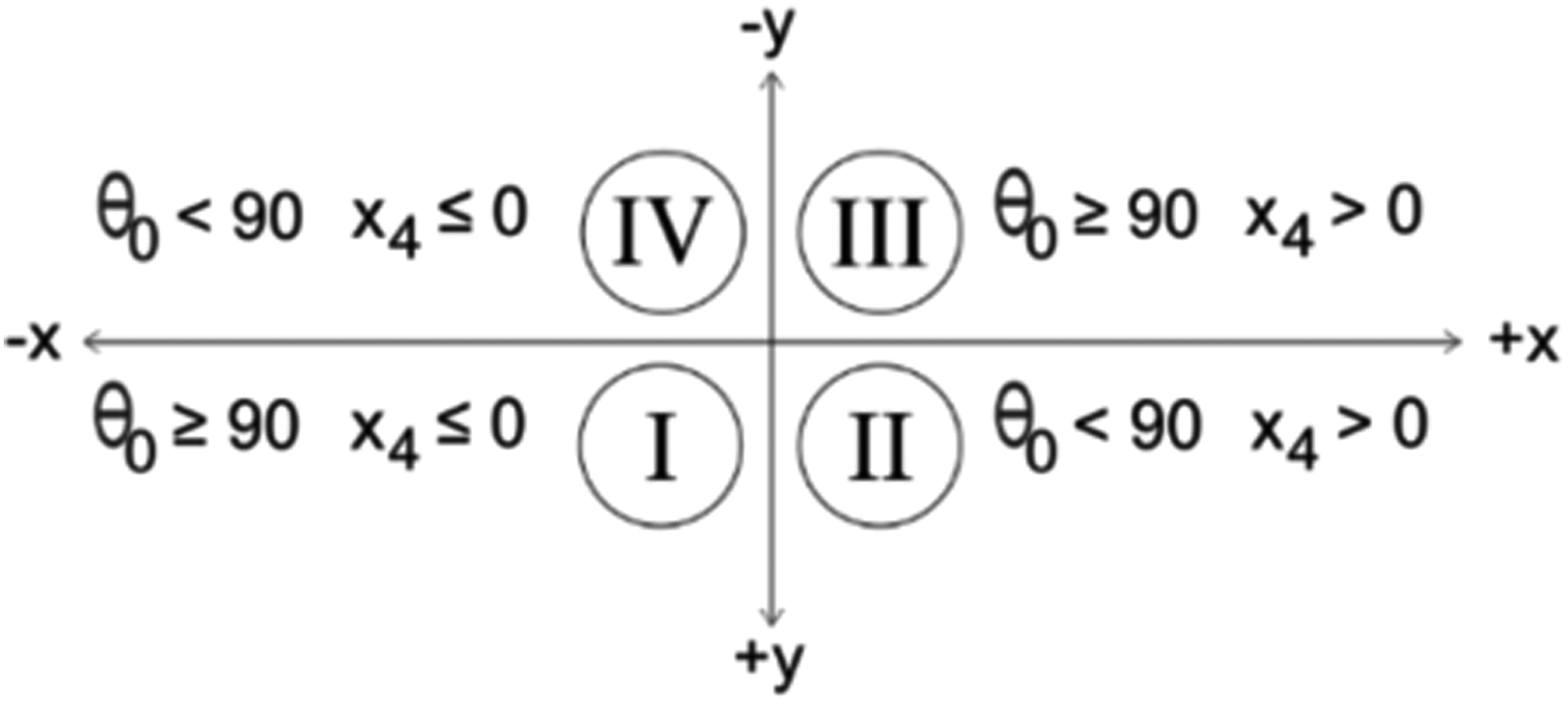
We are trying to find the best location of the point C around the point D (EE point), radius α₄. If a condition $\left|\overrightarrow{AD}\right|<a_2+a_3$ is true, there are 16 options. In order to accelerate the algorithm, the M group enters selections, whose elements from 0 to 8 are switched on/off according to the conditions in the table (Table 2). This means that only a certain number of point C positions are selected depending on the coordinates x′₄ and z₄.

Table 2.

Variety of selected modifications of point C.

Mi	True		Selected points Cx
0	Dx ≥ 0 ∧ Dx ≤ a 4	Dz ≥ 0 ∧ Dz < d 1	C9; C12
1	Dx ≥ 0 ∧ Dx ≤ a 4	Dz < d 1 + a 4	C0; C10,11,12,13,14
2	Dx ≥ 0 ∧ Dx ≤ a 4	Dz ≥ d 1 + a 4	C0,1,2,3,4,5,6,7; C13,14,15
3	Dx ≥ 0 ∧ Dx > a 4	Dz ≥ 0 ∧ Dz < d 1	C0; C10,11,12; C14,15
4	Dx ≥ 0 ∧ Dx > a 4	Dz < d 1 + a 4	C0,1,2; C11; C13,14,15
5	Dx ≥ 0 ∧ Dx > a 4	Dz ≥ d 1 + a 4	C0,1,2,3,4; C13,14,15
6	Dx < 0 ∧ Dx > – a 4	Dz ≥ d 1 ∧ Dz < d 1 + a 4	C15
7	Dx < 0 ∧ Dx ≥ – a 4	Dz ≥ d 1 + a 4	C0,1,2,3,4,5,6,7
8	Dx < 0 ∧ Dx < – a 4	Dz ≥ d 1 + a 4	C1,2,3,4,5,6,7,8,9

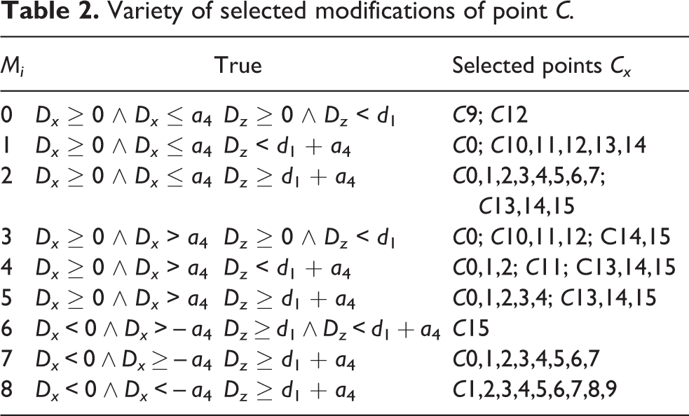
All the possible positions of the point C are shown in Figure 3 (left). In the next step, the calculation method enters only the set of point C positions that satisfy the given selection conditions. If the condition $\left|\overrightarrow{AD}\right|<a_2+a_3$  does not apply, we use the search function for point A and circle with center at point D and radius a ₄. We obtain two or one touch point C, respectively, C′.

Finally, algorithm is used for calculation of rotary angles θ ₁–θ ₄. The algorithm is designed to find the best configuration of calculated rotational angles. The input parameters are the set of variants of point C (further M_C). The algorithm gradually picks out the individual points C _x from the M_C group and looks for the points of the two circles: the first circle has the center at point A and the radius of the arm length a ₂. The second circle has the center at the selected point C_x and the radius of the “elbow” length a ₃. Servomotors of the AL5B robot model have limitations in the range of <0 and 180>°, so we only select the second (farther) contact point B. In the working plane P, we have coordinates of all the necessary points A, B, C, and D. The axis of rotation is perpendicular to the working plane P. The unit vector on the x-axis and the vectors  $\overrightarrow{AB}$ , $\overrightarrow{BC}$ , and $\overrightarrow{CD}$ intersect the searched rotation angles θ ₁–θ ₄. The algorithm evaluates the values of the rotating angles, and in the resulting configuration, it chooses the one in which the angle θ ₂ is the largest and does not include the magnitude of angles outside the servomotor rotation interval.

Data processing of x-IMU sensors

The first step is to create communication between the application and the device—the operator ensures the x-IMU API application environment. The AHRS algorithm needs the right date and time data (x-IMU contains its own AHRS algorithm that, when creating a rotating array, converts data with respect to the Earth’s Centralized fixed reference frame, time-dependent). After sending the current date and time data, it is important to bring the device to the default setting (device reboot). The period T of sensor data is 3.90625 ms and frequency f = 256 Hz. The accelerometer measurement range is set to ± 2 g. Before using the device, we calibrated the accelerometers using the x-IMU GUI program created by the device manufacturer. After restarting the device, the accBias filter is started to reduce the noise of the accelerometer signals. At the same time, another collection of collected data is going into the Kalman filter. Kalman filter outputs (running continuously) are input values to the modified AHRS algorithm (Madgwick AHRS). The advantages are calculating without magnetometer data (in case the magnetometers are not calibrated), further acceleration of the algorithm, and improved accuracy of the output values. The calculated values of the Madgwick AHRS algorithm are used in the implemented original AHRS algorithm for calculating the Euler angles and the rotational matrix R. The signal processing continues by compensating for the acceleration (3) in the reference system with respect to the direction of terrestrial attraction and the linear acceleration (5) in the reference framework.

Next step is the adjustment of the signal by the values obtained by the accBias filter. Adjusted accelerometer data are integrated by time $\Delta t= \frac{1}{256}\hspace{0.17em}\text{s}$ . By the first integration, we get a matrix function of the instantaneous speed (6). By the second integration, we get a matrix positioning function (7). Both results are adjusted using the first-order Butterworth high-pass filter to remove the integration error from the signal. At the end of the data processing cycle, we receive a matrix of coordinate objects in the navigated coordinate system at time Δt.

Accelerometer signal noise reduction method: accBias filter

Based on the theory of relative motion measurements of investigated objects using first and second Newton’s law, we assume that by the method of integration of measured values by time, we can obtain complete knowledge of the velocity and position of objects in the reference coordinate system at a given time. Under real conditions on the earth’s surface, the validity of that assumption is impaired by the impact of forces on IMU sensors. The effort is to eliminate forces using appropriate filters so that the resulting values are close to the values measured under ideal conditions in a no-fatigue condition.

That’s why we have designed an easy-to-use filter for measured accelerometer data called accBias filter. The principle of filtering is based on the use of a sample of data measured over a specified time interval and calculating the maximum value from the sample. This value is deducted from the original signal, resulting in the reduction of noise measured (the filtration is applied throughout the measurement time, i.e., during the motion measurement).

After 100 ms (signal stabilization time), the algorithm is cyclized to collect and store the measured data for 3 s, provided that IMU does not move. If the IMU device moves, the cycle is interrupted and restored when the IMU is stationary. The algorithm records the positive and negative signal values. After 3 s, the measured data are evaluated and the maximum value $\overline{\text{max}}$ is found.

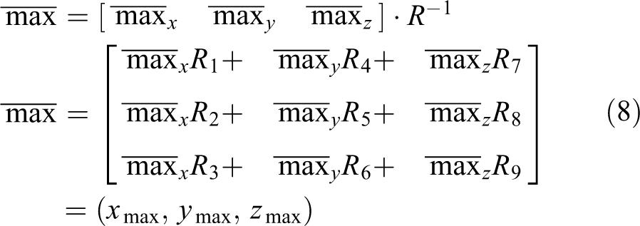
The first operation of the algorithm is to multiply the maximum values by the inverse rotary matrix R ⁻¹ (8) in order to deduct the values from the linear acceleration values (7)

$\begin{array}{l}\overline{\text{max}}=\left[\begin{array}{ccc}{\overline{\text{max}}}_x& {\overline{\text{max}}}_y& {\overline{\text{max}}}_z\end{array}\right]\cdot R^{-1}\\ \overline{\text{max}}=\left[\begin{array}{ccc}{\overline{\text{max}}}_x{R}_1+& {\overline{\text{max}}}_y{R}_4+& {\overline{\text{max}}}_z{R}_7\\ {\overline{\text{max}}}_x{R}_2+& {\overline{\text{max}}}_y{R}_5+& {\overline{\text{max}}}_z{R}_8\\ {\overline{\text{max}}}_x{R}_3+& {\overline{\text{max}}}_y{R}_6+& {\overline{\text{max}}}_z{R}_9\end{array}\right]\\ =\left(x_{\text{max}},y_{\text{max}},z_{\text{max}}\right)\end{array}$

8

The resulting values of the matrix components (9) are divided by the sizes of the individual components of the gravitational acceleration (4)

$\overline{\text{max}}=\left[\begin{array}{c}{x}_{\text{max}}/g_x\\ y_{\text{max}}/g_y\\ z_{\text{max}}/\left(g_z+1\right)\end{array}\right]$

9

The accBias filter algorithm is cyclical. Therefore, we compare output values n_max from the cycle and the previous values. If the output values are larger than the previous ones (valid for the positive signal component) or lower than the previous ones (applies to the negative signal component), the original values are replaced by the output. The matrix of positive bias values $\text{+}\overline{\text{max}}$ or negative values $-\overline{\text{max}}$ is applied when calculating the speed and position. This means that every component of linear acceleration a_lin is determined to be positive or negative. If positive, the corresponding value from matrix $\text{+}\overline{\text{max}}$ (10) is deduced. If negative, the corresponding value from matrix $-\overline{\text{max}}$  (11) is added to it. The variable n expresses the component x, y, or z

$\left(a_{\text{lin}\left(n\right)}\ge 0\right)\Rightarrow a_{\text{lin}\left(n\right)}=a_{\text{lin}\left(n\right)}-n_{\text{max}};n_{\text{max}}\in +\overline{X}$

10

$\left(a_{\text{lin}\left(n\right)}<0\right)\Rightarrow a_{\text{lin}\left(n\right)}=a_{\text{lin}\left(n\right)}+n_{\text{max}};n_{\text{max}}\in -\overline{X}$

11

Motion detection of the x-IMU device in the navigated coordinate system

In the proposed application, we designed a method to detect when the x-IMU device is moving or not moving. The search status parameter is important for the action of the proposed accBias filter, which collects sensor data just at time intervals when the device is motionless—since unwanted forces on the sensors also occur in the still state, they measure the constant flow of data considered to be the main source of errors in calculating speed and position. This means that the calculated speed of the device (which is not moving) is always greater than zero, if the signal noise is not limited.

The principle of the algorithm is based on the estimation of the limit value, with the average values of the accBias filter calculated as input parameters. The average value in the accBias filter is calculated separately from each measured component x, y, and z, using the formula of the arithmetic mean $\overline{x}=\frac{{{\displaystyle \sum }}_{i=1}^n{x}_i}{n}$ , where x_i are the individual measured values and n is the number of measured values. The calculation is continued by multiplying the mean values by the inverse rotary matrix R ⁻¹ (12), then compensating for the gravitational acceleration (13) calculated by the components of the gravitational acceleration (4)

$\overline{x}=\left[\begin{array}{ccc}{\overline{x}}_x& {\overline{x}}_y& x_z\end{array}\right]\cdot R^{-1}=\left[\begin{array}{ccc}{\overline{x}}_x{R}_1+& {\overline{x}}_y{R}_4+& {\overline{x}}_z{R}_7\\ {\overline{x}}_x{R}_2+& {\overline{x}}_y{R}_5+& {\overline{x}}_z{R}_8\\ {\overline{x}}_x{R}_3+& {\overline{x}}_y{R}_6+& {\overline{x}}_z{R}_9\end{array}\right]=\left(x_p,y_p,z_p\right)$

12

$\overline{x}=\left[\begin{array}{c}{x}_p/g_x\\ y_p/g_y\\ z_p/\left(g_z+1\right)\end{array}\right]$

13

Because this algorithm is cyclical, we compare the resulting mean values n _p from the cycle and the previous average values. If the output values are larger than the previous values, the original values are replaced by the output values. The last operation is to calculate the boundary value δ. The program outputs are constant; therefore, we determine the maximum values from the three average values and multiply the result by the constant C in order to achieve the necessary sensitivity of the motion device. Constant C is an empirical magnitude. After a series of attempts with the device, we set it to C = 25 for movements outside the robot model placement. Because the robot model exhibits high vibration of the construction at run time, it is difficult to find the search value C so that the program knows how to detect the movement of the robot while removing the signal noise caused by the vibrations. We chose the value C = 128.

During the constant flow of the linear acceleration data of the device a _lin, the values of its components (a _linx , a _liny , and a _linz ) are compared with the calculated state variable δ. If they are smaller than δ, the program keeps the information “do not move” for each component in the matrix MOVE (0, 0, 0). For example, if the acceleration value in the x-axis direction exceeds the value δ, in the matrix, the corresponding component changes to TRUE and the program retains the information MOVE (1, 0, 0).

If the movement occurs, the program starts recording the linear acceleration values a _lin (measurement during device movement) during the frequency of 2/3 of the frequency of the device. At the end of the cycle, linear acceleration values again averaged and the obtained values were compared with the value d. The “on the move” status of the process is the opposite of the “do not move” status detection process. This means that if the average value of the component is less than the status variable, the corresponding component changes to FALSE in the matrix. If the average value remains larger, the status did not change and the end-of-motion detection cycle continues.

Achieved results

We evaluated the functionality of the proposed data processing process from IMU based on measurements of unfiltered data and their comparison with data modified or calculated values. An important parameter is an instantaneous velocity, which course over time is a good indicator of the proposed solution. In order to explain the course, we need to know the course of linear acceleration calculated in the suggested way.

We conducted testing of motions in approximate directions x, y, and z. We also used outputs from the graphical oscilloscope, modified by the graphical editor. For linear acceleration measurements, the oscilloscope input data were modified to provide a better idea of the functionality of the proposed motion detection system. Each measurement was realized for a separate movement and is not related to other measurements.

Measurement of linear acceleration data

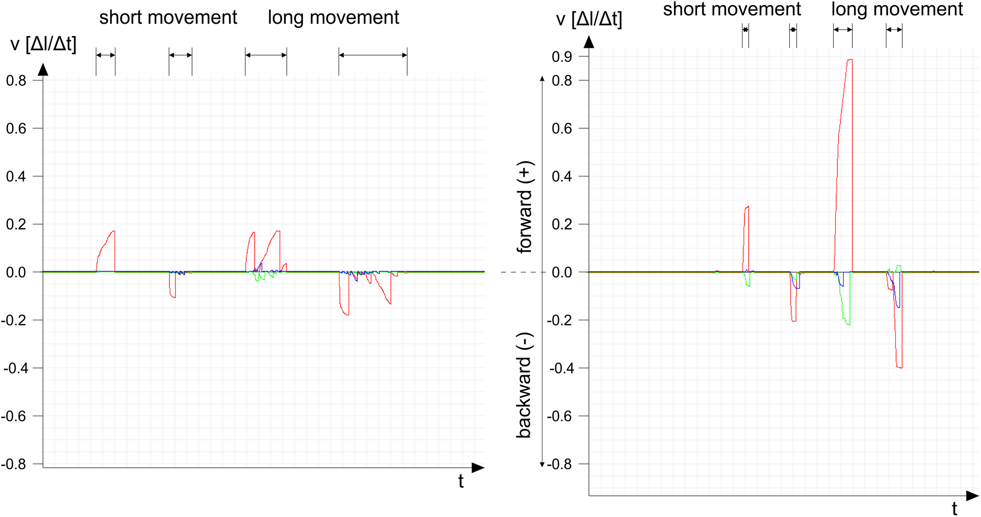
The input data were obtained during the sequence of consecutive movements: (1) short movement in the positive direction, (2) short movement in the negative direction, (3) long movement in the positive direction, and (4) long movement in the negative direction. Limit value δ (red lines) is obtained by the proposed accBias filter algorithm. Calculated linear acceleration values (instantaneous values in the period data collection) are shown in green. The blue color shows their arithmetic average in the period 25 × 3.90625 ms.

In the graph (Figure 5(a)), output values are displayed in the x-axis direction during smooth and slow movements. The system gives fluctuating values (acceleration and subsequent deceleration, twice during smooth motion) with long and slow movements. These findings occur in every measured direction.

Figure 5.

Linear acceleration in the x-axis direction. (a) Slow movements. (b) Fast movements.

In the graph (Figure 5(b)), the output values are displayed in the x-axis during fast movements. The system exhibits a higher degree of accuracy of computed values for fast movements.

This influences the size of the set range and sensitivity of the accelerometers. Gravity and other undesirable forces are naturally neglected with higher acceleration (the approaching range). This phenomenon is of stochastic origin, it cannot be removed by our proposed data processing system, and we consider it the main source of errors in calculating the speed and position.

In the graph (Figure 6(a)), the output values are displayed in the y-axis direction during smooth and slow movements. In the graph, a large number of overshoots can be seen outside the time zones when the device was moving. In several attempts, it was confirmed that the accelerometer system is prone to capture these random fluctuations in measurements, most often in movements in the y-axis direction (possible causes are the fault of the device itself, e.g., slight acceleration of the accelerometer from the axis, in the order of a tenth of a millimeter, release of the platform on which the sensor is anchored).

Figure 6.

Linear acceleration in y-direction. (a) Slow movements. (b) Fast movements.

In the graph (Figure 6(b)), the output values are displayed in the x-axis during fast movements. The values in the graph confirm the assumption of achieving better measurement results at higher accelerations of the device.

In the graph (Figure 7(a)), the output values are displayed in the z-axis direction during smooth and slow movements. Since we measured the hand movements, we assumed that the high uncertainties of the system in the values of linear acceleration (especially in the negative direction) are caused by this factor. In the experimental measurement by placing the IMU on the robot model and the motion control by the application, the system showed a similarly high inaccuracy in the downward direction. The possible cause of this error is the incomplete mathematical model of removing gravitational acceleration from data. The mathematical model used to determine the value of gravitational acceleration (5) uses trigonometric functions—in the vicinity of extremes of functions (sine 0°, cosine 90°), we get high inaccuracies.

Figure 7.

Linear acceleration in z-axis direction. (a) Slow movements. (b) Fast movements.

In the graph (Figure 7(b)), the output values are displayed in the x-axis during fast movements. Measurements in the z-axis direction at high accelerations show the greatest error rate, compared to other measurements. In addition to the accelerometer system, accidental errors described above, and the acceleration orientation error is also shown in the graph.

This means that in the case of rapid movements, the orientation of the first acceleration value (the start of the “moving state”) is negative in terms of the movement being performed. The chart shows the orientation error in long movements, but during repeated attempts, we saw similar results in almost every situation—even with short and fast motions. The possible cause of the error is the design and implementation of the device’s motion detection algorithm. In order to achieve a smooth progress of acceleration values in program time cycles, we programmatically change their orientation according to the first component in the data packet (25 times in the cycle). Assuming that the orientation of the first batch component is correct, the resulting sum of acceleration is consistent with the expected acceleration course. However, if the error of orientation of the first acceleration component occurs, the orientation of the remaining components in the batch is corrected for this error. The final course of the acceleration holds the correct values, but it seems to be deceleration (to calculate the motion speed) in the first phase of movement of the components. Conversely, in the second phase of the movement, acceleration data are transferred to the speed calculation instead of deceleration. It is true that changing the acceleration orientation belongs to stochastic system errors. Therefore, it is difficult to find a suitable way to eliminate the problem for the type of algorithm that collects and processes data in real time. The only possible solution is an inverse algorithm (at least one step back), but in the algorithm thus designed, we lose complete information about the measured quantity.

We identified the possible causes of the errors by analyzing the acceleration values in graphs, where we can also include the use of the designed and implemented accBias filter. The reason is the assumption that any interference with the “raw” data obtained by measurement necessarily causes errors (by rounding the values, by deliberately removing part of the information, etc.). However, if the information intervention is sufficiently sensitive, the errors encountered are within acceptable limits and should not affect the resulting queries.

Measurement of instantaneous speed data

The proposed program for calculating the IMU instantaneous speed of the device in the reference coordinate system receives at the input of the calculated acceleration value. This means that errors identified in previous measurements will also be visible in measured instantaneous speed measurements. In addition, we assume that the presence of an error in the input before integration causes its quadratic increase in the output.

The first graph (Figure 8(a)) shows the values in the x-axis direction during slow movement. The main error directly affects the result of the position calculation. Velocities for long movements are considered the variable velocity. The main error origin is in an identified acceleration error (Figure 5(a)). This causes the instantaneous speeds to reach zero values during a smooth slow movement. This loss of information results in large differences in the calculated and actual location of the device in the space.

Figure 8.

Immediate velocity in the x-axis direction. (a) Slow movements. (b) Fast movements.

The second graph (Figure 8(b)) shows the values in the x-axis direction during fast movement. The result is close to the actual speeds of the device with sufficiently fast movements (with the appropriate acceleration). This results in the correct positioning of the device in space at time t. Assuming that there were no stochastic errors in the time interval of movement or they were sufficiently small.

The graph (Figure 9(a)) shows values in the y-axis direction during slow movement. Similarly, as in the chart description (Figure 6(a)), we note the high inaccuracy of the measured and subsequently calculated acceleration values in the studied direction. This results in the values in the graph being very low—in the application (in the part of the movement display), the position data do not change or change in the given position. It changes very randomly.

Figure 9.

Immediate velocity in the y-direction. (a) Slow movements. (b) Fast movements.

The graph (Figure 9(b)) shows the values in the x-axis direction during fast movement. Based on the values and their course, we can confirm the assumption that in rapid movements with sufficient acceleration andcan calculate the speed and consequently the position. These are very close to real values.

The graph (Figure 10(a)) shows the values in the z-axis direction during slow movement. The greatest deficiency in the given direction of movement is a very frequent change in the actual orientation of the function.

Figure 10.

Immediate velocity in the z-axis direction. (a) Slow movements. (b) Fast movements.

The second major cause of the device positioning errors can also be seen in the last graph (Figure 10(b)). The graph shows that all directions of motions are negative. This means that the first movement upward, at the resulting instantaneous speed, manifested itself as a downward movement. The accelerometer system subsequently evaluated all the movements in the z-axis direction with negative orientations, up to the occurrence of a new random event when the measured orientation did not change again.

Discussion

Based on the design of the INS integration solution for the control and correction of the industrial robot trajectory, we developed an application design that defined three main areas that needed to be further explored to find the right solution.

Assessing the robot model control solution

The robot model control solution was conditional on the movement kinematics study that the device is capable of performing. On the basis of the acquired knowledge, we designed an algorithm for the forward and inverse kinematics of the robot model.

The principle of the forward kinematics algorithm is the calculation of directional vectors in the working plane that passes through the axis of the system of the robot parts (base, shoulder, elbow, and wrist). The input variables are the rotation angles in the robot model’s joints. The searched value is the coordinates of the EE point in the navigated coordinate system.

The principle of the inverse kinematics algorithm is to find the most advantageous position of the point C (position of the last robot model joint) in the working plane. Subsequently, point B (the joint between the shoulder and the elbow of the robot model) is found by the search function of the two circle points. Further, the magnitude of the angles of the robot parts is calculated. The algorithm works with point C modifications. Each configuration of the found points and angles is evaluated in terms of the possibilities of real movements and impacts of parts of the robot model. The best configuration is offered as a solution.

Algorithm suggestions contain shortcomings in the calculation of the robot’s boundary positions. Due to the fact that the purpose of the implementation of the application is to examine the defined hypothesis, the found algorithm deficiencies were not solved further. We designed the test trajectory programs so that the algorithms provide the correct results.

Evaluation of data processing solution for IMU sensors

A necessary condition was the study and understanding of the principles of gyro system, accelerometer, and magnetometers. On the basis of the studied topic, we designed and implemented the process of data from the given sensors. The output value searched for is the instantaneous speed and the derived IMU position in space.

The first step is to implement the proposed accBias filter. The purpose is to minimize the noise from the signal. The principle of filtering is based on obtaining a set of “raw” data for a specified time. Subsequently, the evaluation of the collected data is carried out by finding the maximum values for the positive and negative components. These are used in the data processing process as the values deduced from the calculated linear acceleration. At the same time, the data for calculating the arithmetic mean are collected and evaluated in the algorithm, which is used as a constant variable. The disadvantage of any signal filtering is the loss of complete information about their course over time. On the other hand, the advantage of a given realization is the ability of the program to evaluate the nature of the signal over a time interval and to decide the status of the system “does not move” or “moving.”

The second step is to use data filtered by Kalman filter. We use this modified signal as an input into the Madgwick AHRS algorithm. Outputs are Euler angles and rotary matrix. We obtained the results of the algorithm that we evaluated when testing the application and found that they correspond to the expected values.

The third step of data processing is the calculation of linear acceleration. Calculated results are subtracted from the noise components (accBias filter). Adjusted values are used in the device’s movement detection. At the same time, input variables are used to calculate the instantaneous speed (first integration by time) and then the result is transferred to the input into position calculation (second integration by time).

To test the implemented system, we designed and subsequently performed a set of measurements. Measurements show that the main source of error of the IMU accelerometer system is the stochastic nature and they include:

accidental occurrence of acceleration data measured by the accelerometer in each direction of the navigated coordinate system, regardless of the state of the device (whether or not it is moving) and

accidental change of orientation in the course of measured acceleration values.

Even using an efficient data processing algorithm, its output values are always affected by random input phenomena. An error at the input of the first integration by time causes a quadratic error at the output. If the quadratic error result is used as the input value for the second integration by time, the result contains the cubed error (error raised to the third power). Therefore, in the real-time data processing environment, the proposed solution is unusable. The assumed premise, defined at the beginning of the article, was not confirmed.

Evaluation of the control and correction solution of the programmed trajectory

Since we did not confirm the defined assumption, the implementation of the application contains only a partial solution. There is a prerequisite for doing so to obtain correct position values for EE point. This was not done using the IMU device. The executed program can load the programmed trajectory stored in the external file, can also include tracking control, and would show the values, without track correction.

Conclusion

In the article, we examined the verification of the assumption that the solution for control and correction of the programmed trajectory of the industrial robot by the implementation of INS is possible. Even in the proposed case, INS is used as the sole control device and its data are appropriately processed by the proposed application.

In order to be able to evaluate this assumption, we created a simulation of industrial robot control. As an industrial robot model, we used the AL5B robot model along with the servomotor controller. The INS function in simulation performs an x-IMU device, located at the EE point.

In addition, we designed an application that controls the robot, processes data from the x-IMU device sensors, and calculates the instantaneous speed and location of the x-IMU device in the navigated coordinate system. The application design includes a system for checking and correcting the programmed trajectory.

The defined assumption of the control solution and the correction of the programmed trajectory with the implementation of INS were not confirmed.

Despite the unconfirmed assumption, the implementation of INS in industrial robot management remains an interesting topic for future research. The starting point can be the use for position control (rotation). Main advantage compared to other control systems is the principle of position measurement using the first and second Newton’s law—meaning its use does not require additional adjustments and calibrations during the operation of the industrial robot.