Sage Journals: Discover world-class research

Abstract

This article investigates the capability for backward swimming of a carangiform-fish-like robot with only three joints. A simple dynamic model based on a fixed point, a point in the body without perpendicular oscillation, is first developed to analyze the feasibility of backward motion for the robot. Through this theoretical analysis, we find that the fixed point lies closer to the robotic fish tail with higher backward swimming speeds. Combining the theoretical analysis with experimental optimization, we further explore backward swimming patterns using particle swarm optimization. After a series of online optimal experiments, we find several locomotion gaits that can make the robotic fish swim backward, and the corresponding fixed points are similarly located near the tail. The backward swimming velocity is strongly correlated with the fixed point position along the robotic fish body, which verifies the effectiveness of our fixed-point model.

Keywords

Backward swimming ability fixed-point model optimization robotic fish

Introduction

Autonomous underwater vehicles (AUV) have attracted tremendous attention, as they can be widely applied in oceanography, and in commercial and military missions.^1

–4 However, most existing vehicles can hardly satisfy the increasing requirements expected of them, such as long range, high maneuverability, station keeping or energy saving.⁵ Since most aquatic creatures are endowed with remarkable swimming skills, such as high efficiency, high maneuverability and low noise,⁶ they are an obvious source of inspiration. Therefore, with the development of mechanics, materials, electronics, sensors and controls, enormous strides have been taken in the development of bio-inspired underwater robots over the past two or so decades.^7

–13

Since the first robotic fish was made at MIT,¹⁴ researchers have built a variety of robotic fish.^{15,12,15

–19} Improving the maneuverability of robotic fish is one of the most popular studies in the field, including the development of features such as sharp turning, rolling, front and back flips, and three-dimensional fin undulations.^5,20
–22 Few have considered the backward swimming performance of robotic fish,^21,23

–26 although backward swimming is observed in nature.^27,28 If a robotic fish is endowed with backward swimming ability, its maneuverability will be greatly improved. For instance, when robotic fish swim in narrow spaces or small pipelines, they can only swim backward to go back, as there is not enough space to turn.

To date, the backward swimming of robotic fish has been mainly studied through simulations or experimental optimizations. Using computational fluid dynamics modelling, Anton et al. achieved the backward swimming of a robotic fish with two-link tail.²⁴ Zhou et al. found the backward swimming pattern for a carangiform-fish-like robot based on Lagrangian dynamics. Recently, Yu and Wu optimized the backward swimming patterns of a four-joint robotic fish based on particle swarm optimization (PSO).^21,29 However, finding suitable swimming patterns that make fish swim backward is still quite difficult due to a lack of simple yet general dynamic models and an asymmetric mechanical structure that is propelled forward more easily than backward.

In this article, we first analyze the feasibility of backward swimming for our three-joint robotic fish. A fixed-point (FP) based hydrodynamic model is developed to evaluate the properties of backward motion for our robotic fish. Through this model, we find that it is the position of the FP that determines the velocity of the robot. Whenever the FP is located near the tail, the robotic fish will swim backward, and the fastest backward swimming speed will be achieved when the FP moves to the tip of the tail. Guided by these rules, we present the results of an experimental platform which can automatically optimize the parameters for the backward swimming gaits based on PSO. Several backward swimming patterns were found which further prove the trend relations between backward swimming and FP location which we proposed in the theoretical analysis.

The main contributions of this article are twofold: (1) a simple yet powerful FP-based model is proposed to qualitatively analyze the backward swimming of a carangiform robot; and (2) a combination of the modelling analysis and experimental optimization via PSO is proposed. As a robotic fish is controlled by central pattern generator (CPG) controller, finding the maximum backward swimming control parameters accurately is beyond a simple hydrodynamic model. Experimental optimization without pre-hydrodynamic analysis will consume a lot of time and may converge on sub-optimal results. Here the compromise is that the FP model makes sure that the global optimization, such as the stop condition of the optimization, can be chosen as the tail tip position of the FP, and experimental optimization verifies the effectiveness of the FP model. So the modelling analysis and the experimental analysis supplement each other.

The remainder of the article is organized as follows. Section 2 describes the prototype of a carangiform robot both in mechanism and locomotion controller. The FP hydrodynamic model for the backward swimming analysis of the robotic fish is given in Section 3. An online experimental platform comprising an automatic optimization system for searching for backward swimming gaits is presented in Section 4. In Section 5, results of the experiments are provided. Finally, discussion and an outline of future work are presented in Section 6.

A carangiform robot

Robotic prototype

Figure 1 depicts a wireless-controlled, three-link, carangiform robotic fish prototype developed in our laboratory. The robot is about 0.4 m in length and 0.5 kg in weight. The robotic fish is composed of three parts: rigid head, flexible body and caudal fin. All the propulsion power is produced by the undulation of the flexible body and flapping of the caudal fin. In the rigid head, there is a control unit, battery and balancing weight adjusted for static balance in stationary water. A pair of fixed pectoral fins are designed to keep the body balanced when the robot swims in water. Furthermore, the head is equipped with a wireless communication module which is used for transmitting data between the robotic fish and the upper computer. The flexible body is mainly comprised of three joints and servomotors; these are all covered with a soft but waterproof skin. The caudal fin is made of rubber, and its stiffness decreases towards its end, resembling a real fish.

Figure 1.

The robotic fish is divided into three parts: rigid head, flexible body and caudal fin.

CPG-based locomotion controller

To implement the online optimization of the control parameters, the locomotion controller for the robotic fish should be capable of adapting to any body wave form of fish. A simple, linear, yet still powerful CPG model is applied to control the locomotion of the robotic fish.^30,31 This CPG controller is based on coupled oscillators similar to neural networks in animals, defined as:

{\dot{r}}_{i} (t) = α_{i} (R_{i} - r_{i})

{\ddot{φ}}_{i} (t) = \sum_{j = 1, j \neq i}^{N} μ [μ (φ_{j} (t) - φ_{i} (t) - ϕ_{i j}) - 2 ({\dot{φ}}_{i} (t) - 2 π v)]

θ_{i} (t) = r_{i} (t) \cos (φ_{i} (t))

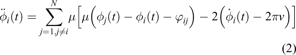
where r_i, φ_i and θ_i represent the amplitude, the phase and the outputs of i th oscillator, respectively. R_i denotes the amplitude setting of the i th oscillator determining the body wave of our robotic fish. Considering that the robot is controlled by the rotation of the severmotor, we scale the amplitude with the maximum rotation angle. ϕ_ij, calculated as φ_j − φ_i, is named the lag angle and represents a bias of phase between oscillators i and j when the oscillators reach stability. In physics, ϕ_ij equals −ϕ_ij, and ϕ_ij = ϕ_ik + ϕ_kj; thus, for three oscillators, two phase biases, such as ϕ₁₂ and ϕ₁₃, can describe all the phase relationships among them. v is the frequency of all the oscillators. Structural parameters α and μ respectively affect the convergence rate of r_i and φ_i. One can refer to Li et al. for a detailed introduction of this CPG controller, including its convergence analysis.³¹

As a basis for the online automatic optimization, the onboard CPG controller is significant. This CPG model is linear, so that it can be easily implemented in AVR controllers. Figure 2 shows a framework of the application of the above CPG controller in our robotic fish. Whenever the robotic fish receives a new group of control parameters from the upper computer, the CPG network first generates the corresponding turning angles for each servomotor. Then the AVR microcontroller transmits these angles as PWM signals, driving the three servomotors. One can refer to the details of the implementation of the CPG controller in the AVR controllers in Li et al.³²

Figure 2.

Framework of CPG controller embedded in the three-link robotic fish.

Fixed point hydrodynamic model

Due to the asymmetric structure of the carangiform robot, it is difficult for the robot to swim backward. The following work aims to determine whether carangiform robots can swim backward through only the undulation of the rear two-thirds of its body. We propose a hydrodynamic model termed the FP model,³³ which is an extension of the classical elongated body theory (EBT).³⁴ This model considers the head shaking and evaluates both forward and backward thrust and swimming speed. According to this model, the carangiform robot exhibits backward swimming abilities when the FP is located in the rear part of the robot.

Description of the body wave

Before we go through the detail of our FP model, we should first introduce the body wave, as it is the basis of EBT and the FP model. The body wave was first defined and systematically researched by Gray.³⁵ He observed that most fish in nature generate thrust through body undulation to overcome the drag of water. Consequently, defining an appropriate body wave function is the first step in the further study of fish swimming for both experimental and theoretical researchers.

Figure 3 gives a top-down view of a carangiform fish body in the earth-fixed inertial reference frame (x, z). The fish swims along the direction of −x, and its perpendicular displacement is described as z(x, t). Further, the body wave function was used to mathematically describe how the fish’s body undulates periodically. Lighthill proposed one of the expressions of the body wave as

Figure 3.

Overhead view of fish body wave defined in the earth-fixed inertial reference frame. There is a discrepancy between the body waves of the fish (dotted line) and robotic fish (solid line).

z (x, t) = (c_{1} x + c_{2} x^{2}) sin (k x + ω t)

where z(x, t) denotes the transverse displacement of fish body, x is the displacement along the main axis, k is expressed as 2π/λ where λ is the body wave length, c₁ and c₂ are linear and quadratic wave amplitude envelopes, respectively, and ω is regarded as the frequency of the body wave.³⁴

Because the oscillation of the man-made robot is achieved through discrete rotating hinge joints, a discrete planar spline curve is taken into account,

z (x_{i}, t) = (c_{1} x_{i} + c_{2} x_{i}^{2}) sin (k x_{i} + ω t)

where i denotes i th joint of robot. Here i equals 1, 2, 3 for our three-joint robotic fish. The robotic fish’s body wave is approximated by the linkages that are driven by the CPG controller, and an explanation of the body wave parameters in view of CPG parameters is given as follows: c₁ and c₂ determine the amplitudes of the three joints in the CPG controller; kx_i denotes the lag angle in the CPG controller; and ω equals the frequency in the CPG controller. The transformation from CPG parameters to body wave parameters is simply deduced through the least squares method (LSM).³³

The fixed point model

The FP model is an extension of EBT which was first proposed by Lighthill in 1960.³⁴ EBT has been widely applied in the bio-fluid-dynamic analysis of the locomotion of elongated fish.³⁶

The model assumes that when thrust equals drag force, fish reach a steady state with a mean speed of U, where the word ‘mean’ refers to the average over one period of fish body undulation. According to EBT, the mean thrust is described as

\bar{T} = {[\frac{m}{2} (\bar{{(\frac{\partial z (x, t)}{\partial t})}^{2}} - U^{2} \bar{{(\frac{\partial z (x, t)}{\partial x})}^{2}})]}_{x = l}

where $\bar{(\cdot)}$ denotes the mean value, l denotes the body length and m is defined as the virtual mass at x = l, calculated as

m = \frac{1}{4} π S_{c}^{2} ρ_{ω} β

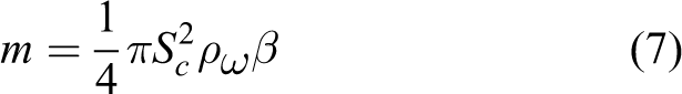
where S_c is the chord length of the tail fin, ρ_ω is the density of the fluid, and β is a nondimensional parameter close to 1. Under inviscid flow conditions, the drag force of a fish is experimentally expressed as

D = \frac{C_{D} ρ_{ω} U^{2} S}{2}

where C_D is a coefficient determined by experiments, and S is the wetted surface area of the undulating part.

When the thrust balances drag, the speed of fish is estimated by

U = {[\sqrt{\frac{m \bar{{(\frac{\partial z (x, t)}{\partial t})}^{2}}}{C_{D} ρ_{ω} S + m \bar{{(\frac{\partial z (x, t)}{\partial x})}^{2}}}}]}_{x = l}

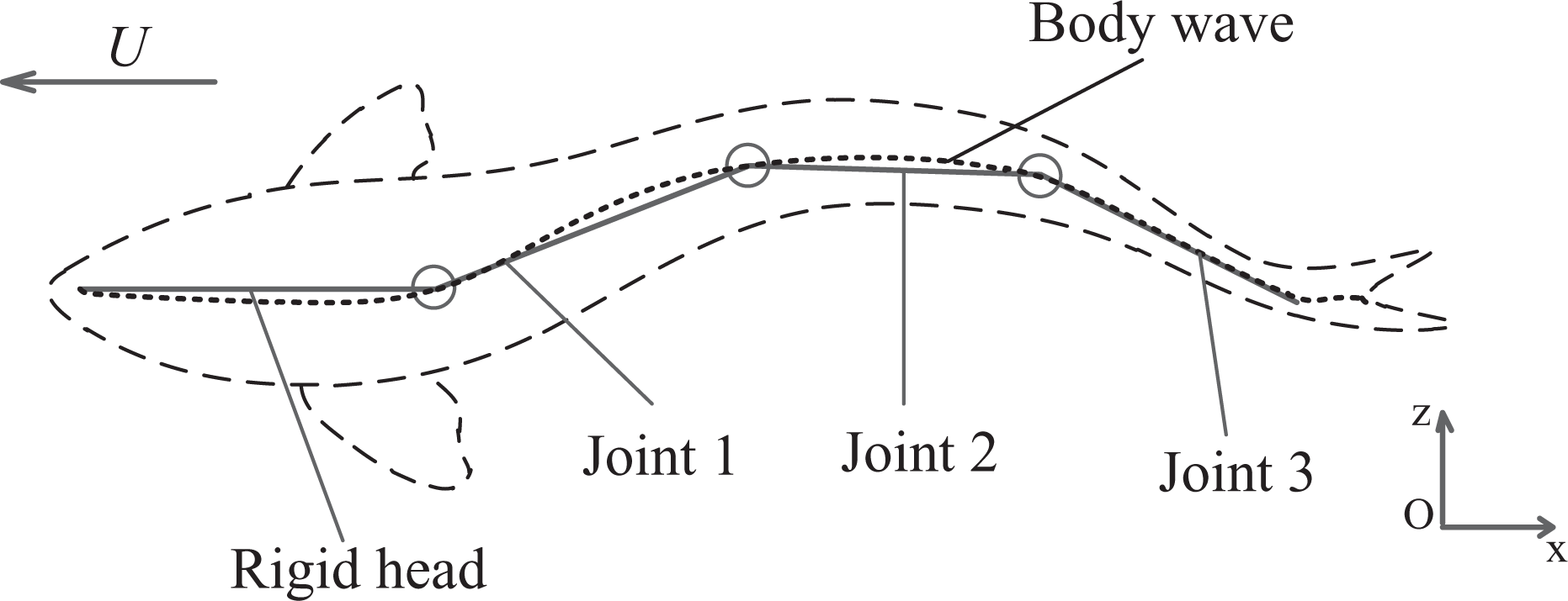
In EBT, a basic assumption is that the rigid head has no displacement in the z axial. However, natural carangiform fish usually swim with body undulation along with head shaking.³⁷ And, according to our previous studies on hydrodynamic modelling,³³ as well as the analysis of the locomotion of fish swimming (see Figure 4), we find that a point in the body of robotic fish instead of its head has no oscillation in z. The position of the point is determined by both the mechanical properties of the fish and its specific body wave. Here, we define these points as fixed-points (FPs) and naturally modify the traditional body wave function as

z' (x, t) = (c_{1} (x - x_{0}) + c_{2} (x^{2} - x_{0}^{2})) sin (k (x - x_{0}) + ω t)

Figure 4.

(a) Successive dorsal profiles of robotic fish swimming at 0.0336 m/s (0.084 BL/s, where BL stands for body length), determined at 1.25s intervals. (b) Images from (a) overlain. A fixed-point is located in the body of robotic fish, and, according to the FP, the fish body is divided into two parts: front and rear.

where x₀ represents the position of the FP. The body undulation of robotic fish can be divided into two parts, separated by FP: front and rear (see Figure 4). The virtual masses of the front and rear parts are recorded as m₁ and m₂, and the thrusts generated by these two parts are calculated as

\bar{T_{1}} = {[\frac{m_{1}}{2} (\bar{{(\frac{\partial z' (x, t)}{\partial t})}^{2}} - U^{2} \bar{{(\frac{\partial z' (x, t)}{\partial x})}^{2}})]}_{x = 0}

\bar{T_{2}} = {[\frac{m_{2}}{2} (\bar{{(\frac{\partial z' (x, t)}{\partial t})}^{2}} - U^{2} \bar{{(\frac{\partial z' (x, t)}{\partial x})}^{2}})]}_{x = l}

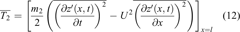
If the thrust of the undulation of the rear part is larger than that of the front, the robotic fish swims forward and its speed is calculated as

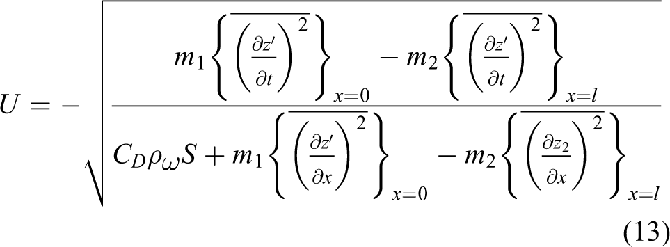
U = - \sqrt{\frac{m_{1} {\bar{{(\frac{\partial z'}{\partial t})}^{2}}}_{x = 0} - m_{2} {\bar{{(\frac{\partial z'}{\partial t})}^{2}}}_{x = l}}{C_{D} ρ_{ω} S + m_{1} {\bar{{(\frac{\partial z'}{\partial x})}^{2}}}_{x = 0} - m_{2} {\bar{{(\frac{\partial z_{2}}{\partial x})}^{2}}}_{x = l}}}

On the contrary, if the thrust generated by the undulation of the front part is larger, the robotic fish swims backward and the speed is derived as

U = \sqrt{\frac{m_{1} {\bar{{(\frac{\partial z'}{\partial t})}^{2}}}_{x = 0} - m_{2} {\bar{{(\frac{\partial z'}{\partial t})}^{2}}}_{x = l}}{- C_{D} ρ_{ω} S + m_{1} {\bar{{(\frac{\partial z'}{\partial x})}^{2}}}_{x = 0} - m_{2} {\bar{{(\frac{\partial z'}{\partial x})}^{2}}}_{x = l}}}

Whenever (13) and (14) have no solution, the thrust generated by the fish’s undulation is smaller than its drag; that is to say, a robotic fish needs an external thrust to counteract its drag.³⁴

Swimming performance evaluation

Here, an evaluation of whether a carangiform robot can swim backward via two-thirds of body undulation is carried out under the assumption that body undulation remains constant while the position of the FP varies. This analysis reveals the main determinant for when the fish swims backward with respect to the position of the FP. The structure parameters in the simulation are chosen according to the physical robotic fish, and are shown in Table 1.

Table 1.

Parameters setting in simulation.

Variable	Value
c ₁	0.2489
c ₂	0.5173 (m ⁻¹)
k	2.938 (rad/m)
ω	1.4 (rad/s)
l	0.4 (m)
S	0.28 (m)
S_c	0.032 (m)
ρ	1000 (kg/m³)
m1	61.575 (g)
m2	12.315 (g)
C_D	0.1309

Thrust and speed of the fish are calculated via (13) or (14) with the position of the FP varying from the head to the tail of the fish. When the FP is located at the head of robot, the robotic fish swims forward with a maximum speed of 0.429 m/s (1.073 BL/s, where BL stands for body length). On the contrary, when the FP goes to the tail tip of the robot, it swims backward with a maximum speed of 0.357 m/s (0.893 BL/s). When the FP equals x_t (see Figure 5), the fish will swim neither forward nor backward. The fish is likely to struggle in the water. The region of the backward swimming gaits is much smaller than that of the forward swimming gaits. This is due to the fact that the virtual masses near the head are much smaller than those near the undulating body for most carangiform robots. Thereby, FPs mostly stay in the forward section of the body, and the robotic fish swims forward more easily than it swims backward.

Figure 5.

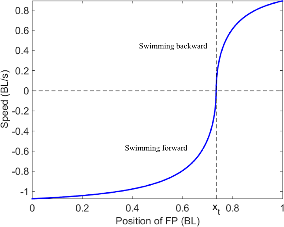
Simulation of speed with the position of the FP ranging from the head to the tail.

Actually, the FP model proves the feasibility of backward swimming for a carangiform robot, and shows that, if we can find gaits that move the FP near the tail, the robot may swim backward. However, it is quite difficult to determine the position of the FP with accuracy using only the model. Therefore, to find a suitable body wave or CPG controller for our robotic fish to swim backward, we found it necessary to carry out some experiments with the real robot. In the following section, we first develop an automated optimization platform for the speed optimization, and, guided by the theoretical analysis, we optimize the control parameters for our robot to swim backward based on PSO.

Experimental platform

According to the above theoretical analysis, backward swimming for a robotic fish is feasible. Thus, in this section, we develop an experimental platform that uses the PSO algorithm to find the control parameters that make the fish swim backward. First, we build a basic experimental platform, including the hardware and software system. We further introduce how to apply the PSO algorithm to find CPG parameters that enable our robotic fish to swim backward as fast as it can.

Test platform

We set up a test platform to find the backward swimming gaits for our robotic fish. The testbed for the experiments consisted of four parts: an upper computer, a wireless transmitter, a global view camera and a swimming tank (see Figure 6). The swimming tank was 300 × 200 cm, with a water height of around 20 cm. A global view camera was equipped above the swimming tank to record videos with a resolution of 800 × 600 pixels and a depth of 8 bit per pixel in real-time.

In the experiments, the upper computer acquires the video data from the camera at 25 fps and calculates the robotic locomotion. After acquiring the information, the upper computer updates the CPG parameters and sends these parameters to the robotic fish via the wireless transmitter. In order to optimize automatically, a software platform wass also developed to provide a user-friendly interface to deal with all the processes of backward swimming optimization, including sending control parameters, handling pattern recognition and updating algorithm optimization. Pattern recognition is vital for our parameter search, since it is used to acquire both the speed and position of robotic fish. In order to do the online tracking, we simply tracked the rigid head instead of the whole deformable robotic fish. A detailed introduction to the test platform we adopted here can be found in Shao and Xie.³⁸

Figure 6.

Experimental Platform.

The particle swarm optimization algorithm

To find the suitable parameters that enable the robotic fish to swim backward, we applied an evolutionary computation algorithm, PSO, to update the CPG control parameters. PSO was first presented by Kennedy and Eberhart in 1995.³⁹ In 1998, in order to overcome local convergence in PSO, Shi et al. proposed a modified PSO algorithm with an inertia weight that plays the role of balancing the global and the local search ability.⁴⁰ Until now, because PSO is simple and powerful, it has been researched and used in many fields, for example in the analysis of human optimization, in examining the metal removal operation in manufacturing environments and in multi-dimensional optimization.

In this article, PSO with inertia weight is applied for the optimization of the backward swimming speed of a a carangiform fish, and this algorithm is described as

V_{i}^{k + 1} = ω_{p} V_{i}^{k} + a_{1} {rand}_{1 i}^{k} ({pbest}_{i}^{k} - P_{i}^{k}) + a_{2} {rand}_{2 i}^{k} ({gbest}^{k} - P_{i}^{k})

P_{i}^{k + 1} = P_{i}^{k} + V_{i}^{k}

where a₁ and a₂ are two positive constants, and rand_1i and rand_2i are two random coefficients in the range of [0, 1]. The subscript i denotes the i th particle. $V_{i}^{k}$ illustrates the velocity of the i th particle in the k th generation. $P_{i}^{k}$ implies the position of the i th particle in the k th generation. ω_p, called inertia weight, represents the influence of the velocity achieved by the last generation. ${pbest}_{i}^{k}$ is the best position of the i th particle during all k generations, and gbest_k denotes the best position of all particles during k generations.

The PSO algorithm is simple but powerful, and it can be easily applied to and implemented in engineering. Before optimization, we only need to initialize ω_p, a₁ and a₂. Moreover, the fitness, as the optimal object, can correlate with whichever variable in the physical system requires optimization. During the optimization, fitness determines which position of the particle is the personal best ( ${pbest}_{i}^{k}$ ) and which one is the global best (gbest_k). Here, we define the fitness in this algorithm as the speed of our robotic fish acquired through the testbed and software system. Therefore, ${pbest}_{i}^{k}$ represents the control parameters that enable fish to swim backward fastest during the k th generation for each particle. And gbest^k represents the control parameters that make the fish swim backward fastest during k th generation for all the particles.

Experimental system

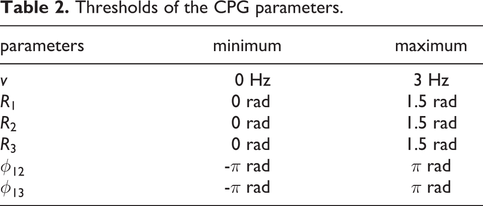
Since the locomotion of robotic fish is controlled by the CPG, we define the position of particle in the PSO algorithm as CPG control parameters [R₁, R₂, R₃, ϕ₁₂, ϕ₁₃, v]. The velocity of each particle represents the variation of each group of CPG parameters. Considering both the guidance of theoretical analysis and the physical limitations for each particle, the parameter spaces for all the particles are bounded. Table 2 presents the thresholds of the PSO parameters. Moreover, similarly to the limited movement abilities of animals in nature, there are maximum and minimum velocities for these particles. Thresholds of particle velocities in this algorithm are also given in Table 3.

Table 2.

Thresholds of the CPG parameters.

parameters	minimum	maximum
v	0 Hz	3 Hz
R ₁	0 rad	1.5 rad
R ₂	0 rad	1.5 rad
R ₃	0 rad	1.5 rad
φ ₁₂	-π rad	π rad
φ ₁₃	-π rad	π rad

Table 3.

Maximum and minimum speed of particles

parameters	minimum velocity	maximum velocity
$\dot{v}$	−0.5 Hz/s	0.5 Hz/s
${\dot{R}}_{1}$	−0.1 rad/s	0.1 rad/s
${\dot{R}}_{2}$	−0.1 rad/s	0.1 rad/s
${\dot{R}}_{3}$	−0.1 rad/s	0.1 rad/s
${\dot{φ}}_{12}$	−0.1π rad/s	0.1π rad/s
${\dot{φ}}_{13}$	−0.1π rad/s	0.1π rad/s

Figure 7 shows a flowchart illustrating how PSO is applied in our experimental platform to find the backward swimming gaits for the robotic fish. Two loops are included in this optimization. One is the inner loop for each particle during one generation, and the other is the outer loop for a swarm of particles in one generation. After each outer loop we will get the real swimming speed for each particle, and ${pbest}_{i}^{k}$ will update based on the comparison between the latest swimming speed and ${pbest}_{i}^{k - 1}$ after each inner loop. In a similar way, gbest^k will update based on the comparison of the latest swimming speed and gbest^k−1 after each outer loop. The programme will stop whenever the iteration reaches the defined maximum value or the deviation between the latest two gbest values is smaller than the setting error.

Figure 7.

Flowchart of the PSO algorithm used in the experiments.

Results

A PSO algorithm with 10 particles was applied to find the CPG parameters for the maximum backward speed. The initialization of the positions was random. The optimization stopped when the number of iterations reached the maximum, or the FP was close enough to the fish tail tip that the fish swam fastest according to the FP model. Here, in order to fully optimize the gaits, we neglect this stop condition.

According to (15) and (16), besides the random initialization of particle positions and speeds, parameters ω_p, a₁ and a₂ also play important roles during the optimization. Since we prefer that particles have more ability of exploration when started, and converge quickly when close to the goal, ω_p is chosen as a simple function of iteration

ω_{p} (i) = ω_{p_{max}} - (ω_{p_{max}} - ω_{p_{min}}) \times \frac{i}{{Iter}_{max}}

where ω_p(i) represents the particles’ inertial value in the i th iteration, and Iter_max is the maximum number of iterations, set as 25 in this experiment. To ensure the algorithm converges quickly, parameters ω_{p
_max}, ω_{p
_min}, a₁ and a₂ are initialized at 0.8, 0.1, 1.5 and 2.0, according to the analysis of Shi et al. and Clerc.^40,41

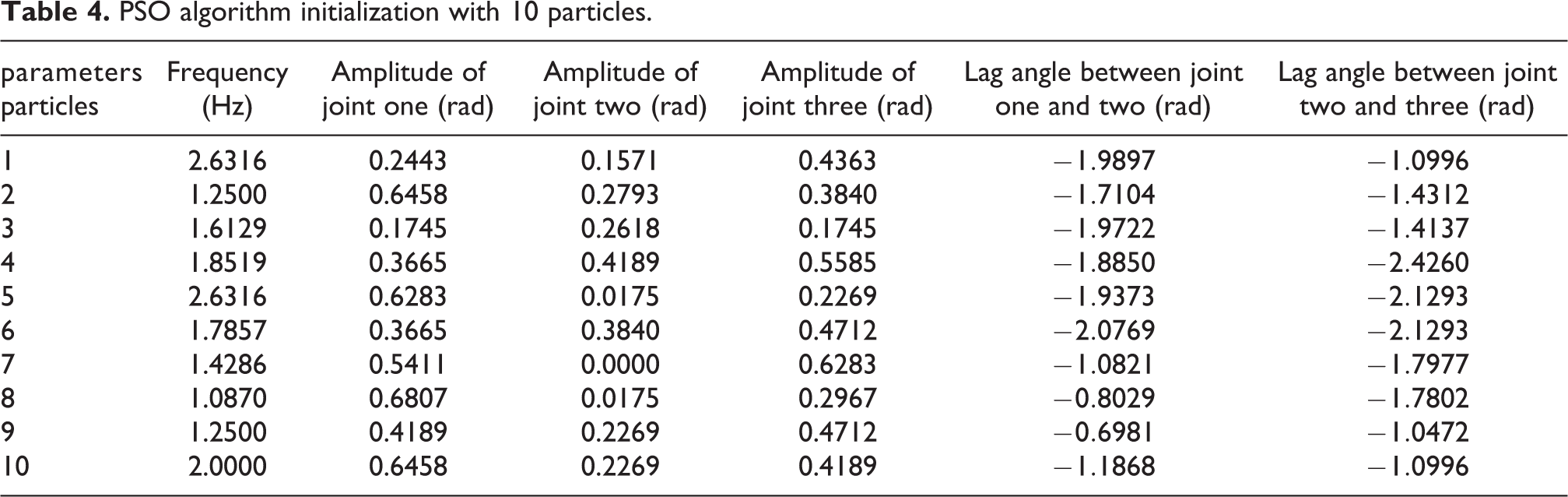
In order to improve the performance of the PSO algorithm, an experiment with 10 particles was designed to find the CPG parameters for backward swimming. The random initialization and experiment results are shown in Table 4 and Figure 8, respectively. Several backward swimming gaits are found as the global best fitness, shown by the red solid line in Figure 8. The maximum backward speed achieved was 0.124 m/s (about 0.31 BL/s). Figure 9 shows comparisons between the experiments and modelling for several backward swimming gaits. Although there are some differences between the experiments and modelling, the trend that the fish swims backward faster when the FP is larger agrees with the prediction of the model. Therefore, the experiments verify the effectiveness of the modelling. A group of snapshots of the robotic fish swimming backward at these parameters is shown in Figure 10. Results prove that there are less CPG parameters that make the robot swim backward, which explains why this mode cannot be found through ‘cut and try’ methods. The corresponding CPG parameters are [R₁, R₂, R₃, ϕ₁₂, ϕ₁₃, v] = [ 0.79, 0.23, 0.44, −0.93, −1.9, 1.6]. All these parameters show that backward swimming needs a large FP. And the larger the FP, the faster the backward swimming. Moreover, as the optimal CPG lag angles are negative, the body envelope of the robotic fish’s backward swimming is essentially the opposite of that of forward swimming. All these experimental results correspond with the conclusion of the FP model that the fish reaches maximum backward swimming speed when the FP is located near the tail.

Table 4.

PSO algorithm initialization with 10 particles.

parameters particles	Frequency (Hz)	Amplitude of joint one (rad)	Amplitude of joint two (rad)	Amplitude of joint three (rad)	Lag angle between joint one and two (rad)	Lag angle between joint two and three (rad)
1	2.6316	0.2443	0.1571	0.4363	−1.9897	−1.0996
2	1.2500	0.6458	0.2793	0.3840	−1.7104	−1.4312
3	1.6129	0.1745	0.2618	0.1745	−1.9722	−1.4137
4	1.8519	0.3665	0.4189	0.5585	−1.8850	−2.4260
5	2.6316	0.6283	0.0175	0.2269	−1.9373	−2.1293
6	1.7857	0.3665	0.3840	0.4712	−2.0769	−2.1293
7	1.4286	0.5411	0.0000	0.6283	−1.0821	−1.7977
8	1.0870	0.6807	0.0175	0.2967	−0.8029	−1.7802
9	1.2500	0.4189	0.2269	0.4712	−0.6981	−1.0472
10	2.0000	0.6458	0.2269	0.4189	−1.1868	−1.0996

Figure 8.

PSO algorithm with 10 particles and a limit of 25 iterations. Each ∗, in varying colours, represents a different particle in the PSO. The fitness value of each iteration is connected with the red line. The blue dash line is the 1 st particle over 25 th iterations. The ∗ s in iteration 0 represent the actual swimming speeds of the particles given the initial CPG parameters described in Table 4.

Figure 9.

Comparisons between experiments and simulations for different FPs.

Figure 10.

Snapshots of robotic fish swimming backward at maximal speed. The time step between the snapshots is 0.5 s.

There are several notes concerning this experimental optimization.

With each initialization of PSO parameters, five repeat experiments were performed in order to reduce accidental errors. The maximum backward swimming speed was defined as the average value of these five experiments.

In order to decrease the mechanical and battery induced discrepancy, all the experiments were performed on the same robotic fish with at least 80 percent of battery power.

Considering the processes of acceleration and deceleration, the speeds of the robotic fish (the fitness in the PSO) are calculated 10 s after (before) the robotic fish started (stopped).

Due to the limitations of actual robotic fish, such as mechanical wear and battery aging, optimizations of the 10 particles were performed in the real robot within 25 iterations. One may find faster backward speeds using the experimental platform with more particles and iterations.

Discussion and conclusion

Through theoretical analysis and experimental optimization, we proved and verified the possibility of backward swimming for a carangiform robot. The theoretical analysis was based on the novel hydrodynamic FP model. In order to find the backward swimming gaits for the physical robot and verify the hypothesis of the model, we carried out a series of experiments on our robot and found a backward swimming gait with a maximum velocity of 0.31 BL/s. The corresponding Reynolds number based on the body length (BL) and the dynamic viscosity ν of water at 30 C is Re = UL/ν = 78, 700, which is the same number as when the robot swims forward with the same speed.⁴² The corresponding Strouhal number is St = fA/U = 1.6 · 0.02/0.31 = 0.1032. The Strouhal number of robot swimming forward at the same speed is evaluated at around St = 0.08. This deviation may be due to the differences of the drag coefficients between forward and backward swimming. When the fish swims forward, the wider rigid head determines the drag coefficient, which is larger than the coefficient when the fish swims backward. Additionally, the head shaking during the fish swimming forward may also cause a higher coefficient for robot swimming forward.

In this article, to find suitable backward swimming gaits, we carried out a feasibility analysis by both modelling and experimental optimization. These two methods supplement each other. The FP-based model proves the feasibility of backward swimming gaits for our robotic fish, and concludes that the FP determines backward swimming performance. Nevertheless, because this model needs FP locomotion before evaluating the swimming speed of robotic fish, we can hardly acquire the backward swimming gaits through this model. While, for the experiments, a stop condition for PSO usually results in a small deviation between the last two steps, this is invalid for the optimization of backward swimming gaits. The control parameter space is so small that the backward swimming speed cannot be improved after several steps (as shown in Figure 8). However, through the relationship between the FP and backward swimming, we find that whenever the FP moves to the end of the tail, the maximum backward swimming speed is achieved. Therefore, the parameter optimization experiments are guided by the theoretical analysis.

Although the backward swimming speed evaluated through the FP model is slightly different from the experimental one, the key feature of backward swimming, that the FP is located in the tail tip when fish swims backward, is definitely the same. The deviations between the experiments and modelling (as shown in Figure 9) may be due to the parameter evaluation in the modelling. For example, the virtual masses for the flapping caudal fin and fish head are time-varying, because of the undulating body. Moreover, the FP model is based on EBT, which ignores the viscosity force, thus resulting in possible deviations. Nonetheless, the trends for both experiments and modelling are the same, thus verifying the effectiveness of the proposal that the larger the FP, the faster the backward swimming speed.

In contrast, natural carangiform fish swim backward mostly by pectoral fin flapping. The reason why natural carangiform fish do not swim backward through body undulation may lie in the high energy cost of that swimming gait. In addition, some natural fish, such as the eel, can also undulate their body to swim backward. The two main features of backward swimming in anguilliform fish are that these fish endowed with large amplitude and high frequency undulations.²⁷ However, our robotic fish only needs small amplitude and moderate frequency. This may result from the different structures between anguilliform and carangiform fish.

Our research will be extended in several directions in the future. First, in order to further improve the maneuverability of the robot, turning will be integrated into the backward swimming of the robotic fish. Second, the proposed architecture will be applied in developing other swimming patterns, such as C-start and minor-radius turning. Finally, we will add some onboard sensors to our robotic fish; thus the robot will accomplish special tasks in some narrow spaces autonomously. For instance, this robotic fish could be applied to the crack detection in under-sea oil pipelines after being equipped with a crack detection device.

Footnotes

Acknowledgement

We would like to acknowledge Stephen Lang for polishing the article.

Declaration of conflicting interests

The author(s) declared no potential conflicts of interest with respect to the research, authorship, and/or publication of this article.

Funding

The author(s) disclosed receipt of the following financial support for the research, authorship and/or publication of this article: This work was supported by the National Natural Science Foundation of China (NSFC, grant numbers 51575005, 61503008, 61633002) and the China Postdoctoral Science Foundation (grant numbers 2015M570013, 2016T90016).

References

Bandyopadhyay

. Trends in biorobotic autonomous undersea vehicles. IEEE J Oceanic Eng 2005; 30(1): 109–139.

Low

. Modelling and parametric study of modular undulating fin rays for fish robots. Mech Mach Theory 2009; 44(3): 615–632.

Tan

. Autonomous robotic fish as mobile sensor platforms: Challenges and potential solutions. Mar Technol Soc J 2011; 45(4): 31–40.

Zhang

Thon

. Miniature underwater glider: Design and experimental results. IEEE/ASME Trans Mechatron 2014; 19(1): 394–399.

Wang

. Control of yaw and pitch maneuvers of a multilink dolphin robot. IEEE Trans Robot 2012; 28(2): 318–329.

Sfakiotakis

Lane

Davies

JBC

. Review of fish swimming modes for aquatic locomotion. IEEE J Oceanic Eng 1999; 24(2): 237–252.

Lauder

Drucker

. Morphology and experimental hydrodynamics of fish fin control surfaces. IEEE J Oceanic Eng 2004; 29(3): 556–571.

Liu

. Biologically inspired behaviour design for autonomous robotic fish. Int J Automat Comput 2006; 3(4): 336–347.

Wen

Wang

. Novel method for the modeling and control investigation of efficient swimming for robotic fish. IEEE Trans Ind Electron 2012; 59(8): 3176–88.

10.

Youcef-Toumi

. Robot fish: Bio-inspired fishlike underwater robots. Berlin Heidelberg: Springer, 2015.

11.

Zhao

Wang

. Vision-based target tracking and collision avoidance for two autonomous robotic fish. IEEE Trans Ind Electron 2009; 56(5): 1401–1410.

12.

Low

Zhou

Zhong

. Gait planning for steady swimming control of biomimetic fish robots. Adv Robot 2009; 23(7–8): 805–829.

13.

Rus

Tolley

. Design, fabrication and control of soft robots. Nature 2015; 521(7553): 467–475.

14.

Triantafyllou

. An efficient swimming machine. Sci Am 1995; 272(3): 64–70.

15.

Wang

Min

. A framework for biomimetic robot fish’s design and its realization. In: Proc Amer control conf, Portland, OR, 8–10 June 2005, pp. 1593–1598. Portland, OR: IEEE.

16.

Liu

Dukes

. Design of swim patterns for autonomous robotic fish. In: Proc IEEE/RSJ int conf intell robots syst, Beijing, China, 9–15 October 2006, pp.2406–2411. Beijing, China: IEEE.

17.

Wen

Liang

Shen

. Hydrodynamic performance of an undulatory robot: Functional roles of the body and caudal fin locomotion. Int J Adv Rob Sys 2013; 10: 10.

18.

Ding

Yang

. Dynamic modelling of a cpg-controlled amphibious biomimetic swimming robot. Int J Adv Rob Sys 2013; 10(199): 1–11.

19.

Wang

Xie

. Online high-precision probabilistic localization of robotic fish using visual and inertial cues. IEEE Trans Ind Electron 2014; 62(2): 1113–1124.

20.

Liu

. Biological inspiration: From carangiform fish to multi-joint robotic fish. J Bionic Eng 2010; 7(1): 35–48.

21.

Tan

. Kinematic comparison of forward and backward swimming and maneuvering in a self-propelled sub-carangiform robotic fish. J Bionic Eng 2014; 11(2): 199–212.

22.

Ren

Yang

Wang

. Hydrodynamics of a robotic fish tail: effects of the caudal peduncle, fin ray motions and the flow speed. Bioinspir & Biomimet 2016; 11(1): 016008.

23.

McIsaac

Ostrowski

. Motion planning for anguilliform locomotion. IEEE Trans Robot Autom 2003; 19(4): 637–652.

24.

Anton

Zheng

Kruusmaa

. Analytical and computational modeling of robotic fish propelled by soft actuation material-based active joints. In: Proc int conf intell robots syst, St. Louis, USA 11–15 October 2009, pp. 2126–2131. New York: IEEE.

25.

Zhou

Cao

Shuo

. The dynamic analysis of the backward swimming mode for biomimetic carangiform robotic fish. In: Proc int conf intell robots syst, Nice, France, 22–26 September 2008, pp. 3072–3076. New York: IEEE.

26.

Zhou

Cao

Hou

. Indeterminate backward swimming gaits for a carangiform robotic fish. Neural Comput & Applic 2012; 23(7): 2015–2021.

27.

D’Aout

Aerts

. A kinematic comparison of forward and backward swimming in the eel Anguilla anguilla . J Exp Biol 1999; 202(11): 1511–1521.

28.

Islam

Zelenin

Orlovsky

Grillner

. Pattern of motor coordination underlying backward swimming in the lamprey. J Neurophysiol 2006; 96(1): 451–460.

29.

Wang

. CPG network optimization for a biomimetic robotic fish via PSO. IEEE T Neural Networ 2015; 27(9): 1962–1968.

30.

Wang

Xie

, Wang L, et al. -based locomotion control of a robotic fish: linear oscillators and reducing control parameters via . Int J Innov Comput I 2011; 7(7B): 4237–4249.

31.

Wang

Xie

. A general network and its implementation on the microcontroller. Neurocomput 2015; 167(2015): 299–305.

32.

Wang

Xie

. Digital implementation of controller in AVR system. In: Proc 33rd Chin control conf, Nanjing, China, 28–30 July 2014, pp. 8293–8298. New York: IEEE.

33.

Wang

Xie

. Modeling of a carangiform-like robotic fish for both forward and backward swimming: Based on the fixed point. In: Proc IEEE int conf robot autom, Hongkong, China, May 31–June 7 2014, pp. 800–805. New York: IEEE.

34.

Lighthill

. Note on the swimming of slender fish. J Fluid Mech 1960; 9(02): 305–317.

35.

Gray

. Studies in animal locomotion. The movement of fish with special reference to the eel. J Exp Biol 1933; 10(1): 88–104.

36.

Sparenberg

. Survey of the mathematical theory of fish locomotion. J Eng Math 2002; 44(4): 395–448.

37.

Dewar

Graham

. Studies of tropical tuna swimming performance in a large water tunnel Kinematics. J Exp Biol 1994; 192: 45–59.

38.

Shao

Xie

. Real-time tracking of moving objects on a water surface. In: Proc IEEE int conf mech autom, Chengdu, China, 5–8 August 2012, pp. 2114–2119. New York: IEEE.

39.

Kennedy

Eberhart

. Particle swarm optimization. In: Proc IEEE int conf neural netw, volume 4, Perth, WA, Australia, 27 November–1 December 1995, pp. 1942–1948. New York: IEEE.

40.

Shi

Eberhart

. A modified particle swarm optimizer. In: Proc IEEE world congr comput intell, Anchorage, AK, USA, 4–9 May 1998, pp. 69–73. New York: IEEE.

41.

Clerc

Kennedy

. The particle swarm—Explosion, stability, and convergence in a multidimensional complex space. IEEE Trans Evol Comput 2002; 6(1): 58–73.

42.

Barrett

Triantafyllou

Yue

DKP

. Drag reduction in fish-like locomotion. J Fluid Mech 1999; 392: 183–212.

Exploring the backward swimming ability of a robotic fish

Abstract

Keywords

Introduction

A carangiform robot

Robotic prototype

CPG-based locomotion controller

Fixed point hydrodynamic model

Description of the body wave

The fixed point model

Swimming performance evaluation

Experimental platform

Test platform

The particle swarm optimization algorithm

Experimental system

Results

Discussion and conclusion

Footnotes

Acknowledgement

Declaration of conflicting interests

Funding

References