Sage Journals: Discover world-class research

Abstract

This article presents the results of the 2-year iroboapp research project that aims at devising path planning algorithms for large grid maps with much faster execution times while tolerating very small slacks with respect to the optimal path. We investigated both exact and heuristic methods. We contributed with the design, analysis, evaluation, implementation and experimentation of several algorithms for grid map path planning for both exact and heuristic methods. We also designed an innovative algorithm called relaxed A-star that has linear complexity with relaxed constraints, which provides near-optimal solutions with an extremely reduced execution time as compared to A-star. We evaluated the performance of the different algorithms and concluded that relaxed A-star is the best path planner as it provides a good trade-off among all the metrics, but we noticed that heuristic methods have good features that can be exploited to improve the solution of the relaxed exact method. This led us to design new hybrid algorithms that combine our relaxed A-star with heuristic methods which improve the solution quality of relaxed A-star at the cost of slightly higher execution time, while remaining much faster than A* for large-scale problems. Finally, we demonstrate how to integrate the relaxed A-star algorithm in the robot operating system as a global path planner and show that it outperforms its default path planner with an execution time 38% faster on average.

Keywords

Robot path planning exact methods heuristic methods large grid environments

Introduction

Motivation

Global path planning is a major component in the navigation process of any mobile robot. It consists of finding a global plan of the path that will be followed by the robot from an initial location to a target location. In the iroboapp project,¹ we addressed the design of intelligent algorithms for mobile robots applications, in particular path planning and multi-robot task allocation problems. In this article, we present the main results of the project in what concerns mobile robot path planning in grid maps. Roughly, the project aims at responding to this general question: Among all existing search techniques and optimization approaches proposed in the literature, what is the best approach to solve the path planning problem? This represents the primary motivation behind this project.

For path planning, our objectives were to (1) investigate existing approaches for solving the path planning problem, (2) evaluate their performance, (3) design new and more efficient approaches, (4) validate through extensive simulations, (5) integrate them into real-world robots and demonstrate their effectiveness. Firstly, we started by analysing the path planning problem and focused on grid map path planning (eight neighbours). In the project, we had particularly addressed large-scale problems with large map sizes, reaching up to 2000 × 2000 grid maps. In fact, although this problem has a polynomial complexity in theory, when the problem size is huge, the execution time of existing fast algorithms (e.g. like A-star (A*)) might be very high. For example, we found out that the average A* execution time on a 2000 × 2000 random obstacle map may reach 296 s on a laptop equipped with an Intel Core i7 processor and an 8 GB RAM.

Problem and solution outline

Analysis of existing literature shows two major approaches commonly used to address the path planning problem: (1) exact methods such as A* and Dijkstra’s algorithms, (2) heuristic methods such as genetic algorithm (GA), tabu search (TS), and ant colony optimization (ACO). Typically, heuristic methods are used in the more general problem, that is, motion planning. It generally pertains to non-deterministic polynomial time hard problems, in particular for robotics arm navigation. However, there has been several attempts to adapt these techniques to grid path planning as well. In fact, Miao et al.² used GA to solve the global path planning in combination with the potential field method. Shu and Fang³ used ACO to solve global and local path planning in U and V-shaped obstacles. These works only addressed small-scale scenarios with map sizes not exceeding 100 × 100, and for most of these cases, it was demonstrated that exact methods perform better.

In this article, we propose a comprehensive comparative study between a large variety of algorithms, both exact and heuristic as well as a relaxed version of A*, used to solve the global path problem. In this work, our concern is not only optimality but also the real-time execution for large problems as this is an important requirement in mobile robots navigation. In fact, we can tolerate some deviation with respect to optimality for the sake of reducing the execution time of the path planning algorithm, since in real robotics applications, it does not harm to generate paths with slightly higher lengths, if they can be generated much faster.

In a first step, we conclude that both exact and heuristic methods are not appropriate for grid path planning and show that relaxed A-star (RA*) is the best path planner as it provides a good trade-off for all metrics. However, heuristic methods have some good features that could be exploited to improve the solution quality of near-optimal relaxed version without inducing extra execution time. Our contribution in this article consists of the design of hybrid algorithms that combine both the RA* algorithm and a selected heuristic method, and we demonstrate their effectiveness through simulation.

Contributions of the article

This article has three major contributions:

We perform a comparative study between exact and heuristic methods and a relaxed version of A*. We conclude that heuristic and exact methods are not appropriate for path planning in large grid maps. We also show that RA* outperforms the other algorithms;

We propose a new hybrid path planners that combine RA* and a heuristic method (GA/TS/ACO);

We integrate RA* planner in the robot operating system (ROS) and show that it outperforms navfn, the default path planner used in ROS.

Related works

Comparative studies of heuristic and exact approaches

To the best of our knowledge, the only previous comparative study of exact and heuristic approaches is the study by Randria et al.⁴ In this article, six different approaches for the global path planning problem were evaluated: breadth-first search, depth-first search, A*, Moore–Dijkstra, neural approach and GA. Three parameters were evaluated: the distance travelled by the robot, the number of visited waypoints and the computational time (with and without initialization). Simulation was conducted in four environments, and it was demonstrated that GA outperforms the other approaches in terms of distance and execution time. Although the presented work evaluates the performance of some exact and heuristics techniques for path planning, there is still a need to evaluate them in large-scale environments as the authors limited their study to small-size environments (up to 40 × 40 grid maps). In this article, we improve on this by considering a vast array of maps of different natures (rooms, random, mazes, video games) with a much larger scale up to 2000 × 2000 cells. Cabreira et al.⁵ presented a GA-based approach for multi-agents in dynamic environments. Variable length chromosomes using binary encoding were adopted to represent the solutions where each gene is composed of three bits to represent a motion direction, that is, up, left, down and so on. The GA performance was compared to that of A* algorithm using simulations with NetLogo platform.⁶ The results show that the A* algorithm highly outperforms the GA, but the GA shows some improvements in the performance when the environment complexity grows. An extension for this work was presented in the work by Cabreira et al.,⁷ where the authors extended their simulations to complex and larger environments (up to 50 × 25) and proposed new operator to improve the GA.

Comparative studies of heuristic approaches

In the literature, some research efforts have proposed and compared solutions for path planning based on heuristic approaches. For instance, a comparative study⁸ between trajectory-based metaheuristic and population-based metaheuristic has been conducted. TS, simulated annealing (SA) and GA were evaluated in a well-known static environment. The experiment was performed in the German University in Cairo campus map. Four evaluation metrics were considered in the experimental study: the time required to reach the optimal path, the number of iterations required to reach the shortest path, the time per each iteration and the best path length found after five iterations. It has been argued that SA outperforms the other planners in terms of execution time, while TS was shown to provide the best solution in terms of path length. Sariff and Buniyamin⁹ used two metaheuristics ACO and GA for solving the global path planning problem in static environments. The algorithms have been tested in three workspaces that have different complexities. Performances between both algorithms were evaluated and compared in terms of speed and number of iterations that each algorithm makes to find an optimal path. It was demonstrated that the ACO method was more effective than the GA method in terms of execution time and number of iterations. Grima et al.¹⁰ proposed two algorithms for path planning, where the first is based on ACO and the second is based on GA. The authors compared between both techniques on a real-world deployment of multiple robotic manipulators with specific spraying tools in an industrial environment. In this study, the authors claimed that both solutions provide very comparable results for small problem sizes, but when increasing the size and the complexity of the problem, the ACO-based algorithm produces a shorter path at the cost of a higher execution time, as compared to the GA-based algorithm. Four heuristic methods were compared in the study by Koceski et al.¹¹: ACO, particle swarm optimization (PSO), GA and a new technique called quad harmony search (QHS) that is a combination between the quad tree algorithm and the harmony search method. The quad tree method is used to decompose the grid map in order to accelerate the search process, and the harmony method is used to find the optimal path. The authors demonstrated through simulation and experiments that QHS gives the best planning times in grid map with a lower percentage of obstacles. The work by Gomez et al.¹² presents a comparison between two modified algebraic methods for path planning in static environments, the artificial potential field method enhanced with dummy loads and Voronoi diagrams method enhanced with the Delaunay triangulation. The proposed algorithms were tested on 25 different cases (start/goal). For all test cases, the system was able to quickly determine the navigation path without falling into local minima. In the case of the artificial potential field method enhanced with dummy loads, the paths defined by the algorithm always avoided obstacles (the obstacles that cause local minima) by passing them in the most efficient way. The algorithm creates quite short navigation paths. Compared with Voronoi, this algorithm is computationally more expensive, but it finds optimal routes in 100% of the cases.

Comparative studies of exact methods

Other works compared solutions based on exact methods. Cikes et al.¹³ presented a comparative study of three A* variants: D*, two-way D* (TWD*) and E*. The algorithms have been evaluated in terms of path characteristics (path cost, the number of points at which path changes directions and the sum of all angles accumulated at the points of path direction changes), the execution time and the number of iterations of the algorithm. They tested the planners on three different environments. The first is a grid map randomly generated of size 500 × 500, the second is a 165 × 540 free map and the third is a 165 × 540 realistic map. The authors concluded that E* and TWD* produce shorter and more natural paths than D*. However, D* exhibits shorter runtime to find the best path. The interesting point of this article is the test of the different algorithms on a real-world application using Pioneer 3DX mobile robot. The authors claimed that the three algorithms have a good real-time performance. Haro and Torres¹⁴ tackled the path planning problem in static and dynamic environments. They compared three different methods: a modified bug algorithm, the potential field method and the A* method. The authors concluded that the modified bug algorithm is an effective technique for robot path planning for both static and dynamic maps. A* is the worst technique as it requires a large computational effort. Eraghi et al.¹⁵ compared A*, Dijkstra and HCTLab research group’s navigation algorithm (HCTNav) that have been proposed in the study by Pala et al.¹⁶ HCTNav algorithm is designed for low resources robots navigating in binary maps. HCTNav’s concept is to combine the shortest-path search principles of the deterministic approaches with the obstacle detection and avoidance techniques of the reactive approaches. They evaluated the performance of the three algorithms in terms of path length, execution time and memory usage. The authors argued that the results in terms of path length of the three algorithms are very similar. However, HCTNav needs less computational resources, especially less memory. Thus, HCTNav can be a good alternative for navigation in low-cost robots. In the work by Duchon et al.,¹⁷ both global and local path planning problems are tackled. The authors compared five different methods: A*, focused D*, incremental Phi*, Basic Theta* and jump point search (JPS). They concluded that the JPS algorithm achieves near-optimal paths very quickly as compared to the other algorithms. Thus, if the real-time character is imperative in the robot application, JPS is the best choice. If there is no requirement of a real time and the length of path plays a big role, then Basic Theta* algorithm is recommended. Focused D* and incremental Phi* are not appropriate for static environments. They can be used in dynamic environments with a small amount of obstacles. Chiang et al.¹⁸ compared two path planning algorithms that have the same computational complexity O(nlog(n)) (where n is the number of grid point): the fast marching method (FMM) and A*. They tested the two algorithms on grid maps of sizes 40 × 40 up to 150 × 150. The authors claimed that A* is faster than the other planners and generates continuous but not smooth path, while FMM generates the best path (smoothest and shortest) as the resolution of the map gets finer and finer. Other research works addressed the path planning problem in unknown environments. Zaheer et al.¹⁹ made a comparison study of five path planning algorithms in unstructured environments (A*, RRT, PRM, artificial potential field (APF) and the proposed free configuration eigenspaces (FCE) path planning method). They analysed the performance of the algorithms in terms of computation time needed to find a solution, the distance travelled and the amount of turning by the autonomous mobile robot and showed that the PRM technique provides a shorter path than RRT but RRT is faster and produces a smooth path with minimum direction changes. A* generates an optimal path but its computational time is high and the clearance space from the obstacle is low. The APF algorithm suffers from local minima problem. In case of FCE, the path length and turning value are comparatively larger than all other methods. The authors considered that in case of planning in unknown environments, a good path is relatively short, keeps some clearance distance from the obstacles and is smooth. They concluded that APF and the proposed FCE techniques are better with respect to this attributes. Al-Arif et al.²⁰ evaluated the performance of A*, Dijkstra and breadth-first search to find out the most suitable path planning algorithm for rescue operation. The three methods are compared for two cases: for one starting one-goal cells and for one starting multi-goal cells in 256 × 256 grid in terms of path length, number of explored nodes and CPU time. A* was found to be the best choice in case of maps containing obstacles. However, for free maps, breadth-first search is the best algorithm for both cases (one starting one-goal cell and one starting multi-goal cells) if the execution time is the selection criteria. A* can be a better alternative if the memory consumption is the selection criteria.

Path planners under study

We have proposed and designed carefully the iPath library²¹ that provides the implementation of several path planners according to the following two classes of methods:

Heuristic methods

Exact methods

The iPath library is available as open source on GitHub under the GNU GPL v3 license. The documentation of Application Programming Interface (API) is available in http://www.iroboapp.org/ipath/api/docs/annotated.html.²²

Heuristic methods

The TS algorithm

In the study by Chaari et al.,²³ we proposed a TS-based path planner (TS-PATH). We adapted and applied the different theoretical concepts of the TS approach to solve the path planning problem in grid map environments. The TS-PATH algorithm starts with an initial path generated randomly using the greedy approach. Then, it attempts iteratively to improve the current path around an appropriately defined neighbourhood until a predefined termination criterion is satisfied. Each neighbour path is reached from the current path by applying a small transformation called move, and we consider three different moves in TS-PATH: insert move, remove move and swap move. Before accepting a new move, we must verify that it improves the current solution and also that the move is not tabu. To avoid being trapped at a local optimum and backtracking to already visited paths, the TS approach keeps track of the recent moves in a temporary buffer referred to as tabu list. Two tabu lists are considered in TS-PATH: TabuListIn and TabuListOut. TabuListIn contains the edges that are added to a path after carrying out a move and TabuListOut contains the edges that are removed from the path after performing a move. A move that exists in a tabu list is considered a tabu move. To avoid the search stagnation during a certain number of consecutive iterations, we designed a new method of diversification to guide the search towards new paths that are not explored. The diversification begins with drawing a straight line between the start and the goal positions. At the radius of N cells (N is a random parameter), the algorithm chooses a random intermediate cell, which will be used to generate a new feasible path from the start to the goal cells across it. The new generated path will be used as an initial solution to restart the TS.

The GA

The second proposed path planner is GA.²⁴ The first step of GA consists of generating an initial population of chromosomes. Each chromosome represents a path. The robot path is encoded as a sequence of free cells. It begins at a start cell and finishes with the goal cell joined by a set of intermediate cells. To generate the initial population, we start with generating an initial path using a greedy approach based on Euclidean distance heuristic. To generate the remaining paths in the initial population, the algorithm will choose a random intermediate cell, not in the initial path, which will be used to generate a new path from start to goal cells across the selected intermediate cell. After the generation of the initial population, each path is evaluated and ranked. The fittest paths are selected to form the current generation. Two selection strategies were used in the GA: elitist selection and rank selection. In each iteration, the paths selected undergo two genetic operators called crossover and mutation. We implemented three different crossover operators: one point, two points and a modified crossover presented in the work by Chaari et al.,²⁵ in order to compare between them and choose the best operator. These steps are repeated until achieving the termination condition.

The ACO algorithm

The third proposed algorithm is the ACO algorithm.²⁶ In nature, ants wander randomly, and upon finding food return to their colony while laying down a chemical substance called pheromone. If other ants find such a path, they are likely not to keep travelling at random but instead to follow the trail, returning and reinforcing it. Over time, the quantity of pheromone is intensified on shorter paths as they become more traversed than longer ones. Within a fixed period, the pheromone trail evaporates. Pheromone evaporation also has the advantage of avoiding the convergence to a local optimal solutions.

In the solution construction phase, each ant is firstly positioned on the start position and then it moves from one cell to another to construct its own path. Before moving to the next cell, the probabilities of candidate neighbour cells are calculated using the pheromone rule probability that takes into consideration two values: the pheromone trail amount τ and the heuristic information η. When the ants finish constructing their paths, the pheromone trails are updated by the ants that have constructed paths. So, the edges belonging to constructed paths will gain more pheromone than others. Additionally, evaporation mechanism causes pheromone decrease at some edges which are not in the paths.

The neural network algorithm

The Hopfield-type neural network (NN) presented in the study by Glasius et al.²⁷ consists of a large collection of identical processing units (neurons), arranged in a d-dimensional cubic lattice, where d is the number of degrees of freedom of the robot. This lattice coincides with the grid representation of the state space such that each state (including obstacles) is represented by a neuron. The neurons are connected only to their z nearest neighbours (where z = 4 or 8, for a 2-dimensional workspace) by excitatory and symmetric connections T_ij. The initial state q_init and the target state q_targ are represented by one node each. The obstacles are represented by neurons whose activity is clamped to 0, while q_targ is clamped to 1. All other neurons have variable activity i between 0 and 1 that changes due to inputs from other neurons in the network and due to external sensory input. The total input u_i to the neuron i is a weighted sum of activities from other neurons and of an external sensory input I_i

u_{i} = \sum_{j}^{N} T_{j i} σ_{j} (t) + I_{i}

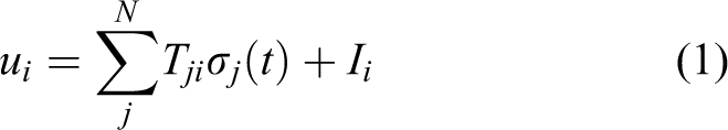
where T_ij is the connection between neuron i and neuron j and N is the total number of neurons. These connections are excitatory (T_ij > 0), symmetric (T_ij = T_ji) and short range

T_{i, j} = {\begin{array}{r} 0 & if & ρ (i, j) < r \\ 1 & otherwise \end{array}}

where ρ(i,j) is the Euclidean distance between neurons i and j. In the case of time-discrete evolution, the activity of a neuron i (excluding the target and obstacles) is updated according to the following equation

σ_{i} (t + 1) = g (\sum_{j}^{N} T_{j i} σ_{j} (t) + I_{i})

where g is a transition function that can be a sigmoid or simply a linear function:

β being the maximum number of neighbours. It is rigorously proven in the study by Glasius et al.²⁷ that, with the above conditions, the network dynamics converges to an equilibrium. The obtained path leads from one node of the lattice to the neighbouring node with the largest activity and ends at the node with activity 1 (q_target). The number of steps and the length of the path obtained are proven to be minimal.

Exact methods

The A* algorithm

The A* algorithm is a path finding algorithm introduced in the study by Hart et al.²⁸ It is an extension of Dijkstra’s algorithm. A* achieves better performance (with respect to time), as compared to Dijkstra, by using heuristics. In the process of searching the shortest path, each cell in the grid is evaluated according to an evaluation function given by

f (n) = h (n) + g (n)

where g(n) is the accumulated cost of reaching the current cell N from the start position S

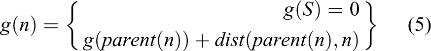
g (n) = {\begin{array}{r} g (S) = 0 \\ g (p a r e n t (n)) + d i s t (p a r e n t (n), n) \end{array}}

h(n) is an estimate of the cost of the least path to reach the goal position G from the current cell N. The estimated cost is also called heuristic. h(n) can be defined as the Euclidian distance from N to G. f(n) is the estimation of the minimum cost among all paths from the start cell S to the goal cell G. The tie-breaking technique is used in our implementation. The tie-breaking factor tBreak multiplies the heuristic value (tBreak*h(n)), when it is used the algorithm favours a certain direction in case of ties. If we do not use tie-breaking, the algorithm would explore all equally likely paths at the same time, which can be very costly, especially when dealing with a grid environment. The tie-breaking coefficient is equal to

t B r e a k = 1 + 1 / (l e n g t h (G r i d) + w i d t h (G r i d))

The algorithm relies on two lists: The open list is a kind of a shopping list. It contains cells that might fall along the best path but may be not. Basically, this is a list of cells that need to be checked out.

The closed list contains the cells already explored.

Each cell saved in the list is characterized by five attributes: ID, parentCell, g_cost, h_cost and f_cost.

The search begins by expanding the neighbour cells of the start position S. The neighbour cell with the lowest f_cost is selected from the open list, expanded and added to the closed list. In each iteration, this process is repeated. Some conditions should be verified while exploring the neighbour cells of the current cell, a neighbour cell is

Ignored if it already exists in the closed list.

If it already exists in the open list, we should compare the g_cost of this path to the neighbour cell and the g_cost of the old path to the neighbour cell. If the g_cost of using the current cell to get to the neighbour cell is the lower cost, we change the parent cell of the neighbour cell to the current cell and recalculate g, h and f costs of the neighbour cell.

This process is repeated until the goal position is reached. Working backwards from the goal cell, we go from each cell to its parent cell until we reach the starting cell (the shortest path in the grid map is found).

The RA* algorithm

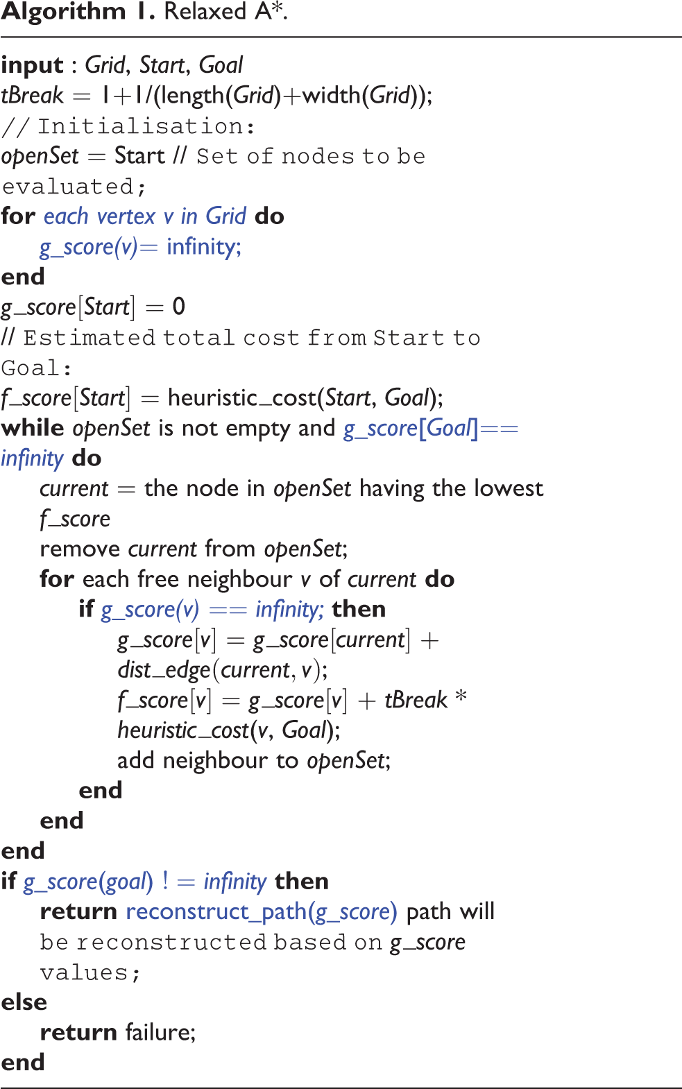
RA* is a new linear time relaxed version of A*. It is presented in the study by Ammar et al.²⁹ It is proposed to solve the path planning problem for large-scale grid maps. The objective of RA* consists of finding optimal or near-optimal solutions with small deviation from optimal solutions, but at much smaller execution times than traditional A*. The core idea consists of exploiting the grid map structure to establish an accurate approximation of the optimal path, without visiting any cell more than once.

In fact, in A*, the exact cost g(n) of a node N may be computed many times; namely, it is computed for each path reaching node N from the start position. However, in the RA* algorithm, g(n) is approximated by the cost of the minimum move path from the start cell to the cell associated with node N.

In order to obtain the relaxed version RA*, some instructions of A* that are time consuming, with relatively low gain in terms of solution quality, are removed. In fact, a node is processed only once in RA*, thus avoiding to use the closed set of the A* algorithm. Moreover, in order to save time and memory, we do not keep track of the previous node at each expanded node. Instead, after reaching the goal, the path can be reconstructed, from goal to start by selecting, at each step, the neighbour having the minimum g(n) value. Also, it is useless to compare the g(n) of each neighbour to the g(n) of the current node N as the first calculated g(n) is considered definite. Finally, it is not needed to check whether the neighbour of the current node is in the open list. In fact, if its g(n) value is infinite, it means that it has not been processed yet and hence is not in the open list. The RA* algorithm is presented in algorithm 1. Both terms g(n) and h(n) of the evaluation function of the RA algorithm are not exact, thus there is no guarantee to find an optimal solution.

Algorithm 1.

Relaxed A*.

input : Grid, Start, Goal

tBreak = 1+1/(length(Grid)+width(Grid));

// Initialisation:

openSet = Start // Set of nodes to be

evaluated;

for each vertex v in Grid do

g_score(v)= infinity;

end

$g_s c o r e [S t a r t]$ = 0

// Estimated total cost from Start to

Goal:

$f_s c o r e [S t a r t]$ = heuristi_cost(Start, Goal);

while openSet is not empty and g_score[Goal]==

infinity do

current = the node in openSet having the lowest

$f_score$

remove current from openSet;

for each free neighbour v of current do

if g_score(v) == infinity; then

$g_s c o r e [v]$ = $g_s c o r e [c u r r e n t]$ +

$d i s t_e d g e (c u r r e n t, v)$ ;

$f_s c o r e [v]$ = $g_s c o r e [v]$ + $t B r e a k$ *

$h e u r i s t i c_c o s t$ (v, Goal);

add neighbour to $o p e n S e t$ ;

end

if g_score(goal) $! =$ infinity then

return reconstruct_path(g_score) path will

be reconstructed based on $g_s c o r e$

values;

else

return failure;

end

Comparative study

Simulation environments

To perform the simulations, we implemented the iPath C++ library²¹ that provides the implementation of several path planners including A*, GA, TS, ACP and RA*. The iPath library is implemented using C++ under Linux OS. It is available as open source on GitHub under the GNU GPL v3 license. The documentation of API is available in http://www.iroboapp.org/ipath/api/docs/annotated.html.²² A tutorial on how to use iPath simulator is available in http://www.iroboapp.org/index.php?title=IPath.³⁰

The library was extensively tested under different maps including those provided in the benchmark³¹ and other randomly generated maps.³² The benchmark used for testing the algorithms consists of four categories of maps:

Maps with randomly generated rectangular shape obstacles: This category contains two (100 × 100) maps, one (500 × 500) map, one (1000 × 1000) map and one (2000 × 2000) map with different obstacle ratios (from 0.1 to 0.4) and obstacle sizes (ranging from 2 to 50 grid cells).

Mazes: All maps in this set are of size 512 × 512. We used two maps that differ by the corridor size in the passages (1 and 32).

Random: We used two maps of size 512 × 512.

Rooms: We used two maps in this category with different room sizes (8 × 8 and 64 × 64). All maps in this set are of size 512 × 512.

Video games: We used one map of size 512 × 512.

The simulation was conducted on a laptop equipped with an Intel Core i7 processor and an 8 GB RAM. For each map, we conducted 5 runs with 10 different start and goal cells randomly fixed. This makes 600 (12 × 5 × 10 maps) total runs for each algorithm.

Simulation results

In this section, we present the simulation results relative to the evaluation of the efficiency of the five different planners. Figures 1 and 2 depict the box plot of the average path costs and average execution times for the randomly generated maps and the benchmarking maps, respectively, with different start and goal cells. Figure 3 shows the average path cost and the average execution time of all the maps. On each box, the central mark is the median, the edges of the box are the 25th and 75th percentiles. Tables 1 and 2 present the average path costs and average execution times for the different maps. Table 3 presents the percentage of extra lengths of the different algorithms in different types of maps, and Table 4 presents the percentage of optimal paths found by the algorithms.

Figure 1.

Box plot of the average path costs and the average execution times (log scale) in 100 × 100, 500 × 500 and 1000 × 1000 random maps of heuristic approaches, tabu search, genetic algorithms and neural network as compared to A* and RA*. A*: A-star; RA*: relaxed A-star.

Figure 2.

Box plot of the average path costs and the average execution times (log scale) in 512 × 512 random, 512 × 512 rooms, 512 × 512 video games and 512 × 512 mazes maps of heuristic approaches tabu search, genetic algorithms and neural network as compared to A* and RA*. A*: A-star; RA*: relaxed A-star.

Figure 3.

Box plot of the average path costs and the average execution times (log scale) in the different maps (randomly generated and those of benchmark) of heuristic approaches tabu search, genetic algorithms and neural network as compared to A* and RA*. A*: A-star; RA*: relaxed A-star.

Table 1.

Average path cost (grid units) for the different algorithms per environments size.

Algorithm	100 × 100	500 × 500	1000 × 1000	2000 × 2000	Random (512 × 512	Rooms (512 × 512)	Video games (512 × 512)	Mazes (512 × 512)
A*	66.2	273.8	473.4	1366.4	303.4	310.6	243.6	1661.9
RA*	70.5	277.0	477.7	1443.3	319.5	341.8	257.8	1687.1
GA	75.3	293.3	476.8	–	360.8	408.7	269.9	–
TS	69.6	335.9	541.1	–	322.9	322.9	531.7	–
NN	82.3	282.8	487.2	–	485.4	322.9	253.1	–

A*: A-star; RA*: relaxed A-star; GA: genetic algorithm; TS: tabu search; NN: neural network.

Table 2.

Average execution times (microseconds) for the different algorithms per environment size.

Algorithm	100 × 100	500 × 500	1000 × 1000	2000 × 2000	Random (512 × 512	Rooms (512 × 512)	Video games (512 × 512)	Mazes (512 × 512)
A*	114	9196	102,647	296,058,499	17,626	62,753	11,761	3,161,774
RA*	17	67	271	15,414	299	834	78	2435
GA	9687	34,405	20,329	–	2,587,005	849,645	39,462	–
TS	544	23,270	39,130	–	58,605	144,768	110,478	–
NN	688	27,713	321,630	–	26,211	62,599	13,802	–

A*: A-star; RA*: relaxed A-star; GA: genetic algorithm; TS: tabu search; NN: neural network.

Table 3.

Percentage of extra length compared to optimal paths calculated for non-optimal paths.

Algorithm	100 × 100 (%)	500 × 500 (%)	1000 × 1000 (%)	2000 × 2000 (%)	Random (512 × 512; %)	Rooms (512 × 512; %)	Video games (512 × 512; %)	Mazes (512 × 512; %)
A*	0.0	0.0	0.0	0.0	0.0	0.0	0.0	0.0
RA*	6.99	0.4	1.97	6.81	5.48	10.13	5.95	2.356
GA	13.68	10.42	1.55	–	16.1	40.48	12.9	–
TS	35.74	17.7	13.06	–	47.31	51.75	26.82	–
NN	5.06	3.2	3.44	–	7.32	3.75	4.3	–

A*: A-star; RA*: relaxed A-star; GA: genetic algorithm; TS: tabu search; NN: neural network.

Table 4.

Percentage of optimal paths per environment size.

Algorithm	100 × 100 (%)	500 × 500 (%)	1000 × 1000 (%)	2000 × 2000 (%)	Random (512 × 512; %)	Rooms (512 × 512; %)	Video games (512 × 512; %)	Mazes (512 × 512; %)
A*	100	100	100	100	100	100	100	100
RA*	5	40	60	10	5	0	20	55
GA	10	50	60	–	10	0	30	–
TS	5	0	0	–	5	0	0	–
NN	5	10	20	–	5	0	0	–

A*: A-star; RA*: relaxed A-star; GA: genetic algorithm; TS: tabu search; NN: neural network.

We can conclude from these figures that the algorithms based on heuristic methods are in general not appropriate for the grid path planning problem. In fact, we observe that these methods are not as effective as RA* and A* for solving the path planning problem, since the latter always exhibit the best solution qualities and the shortest execution times.

Although GA can find optimal paths in some cases as shown in Table 4, it exhibits higher runtime as compared to A* to find its best solution. Moreover, non-optimal solutions have large gap 15.86% of extra length on average as depicted in Figure 4. This can be explained by two reasons: The first reason is that GA needs to generate several initial paths with the greedy approach, and this operation itself takes time which is comparable to the execution of the whole A* algorithm. The second reason is that GA needs several iterations to converge, and the number of iterations depends on the complexity of the map and the positions of the start and goal cells.

Figure 4.

Average percentage of extra length compared to optimal path, calculated for non-optimal paths.

The TS approach was found to be the least effective. It finds non-optimal solutions in most cases with large gaps (32.06% as depicted in Figure 4). This is explained by the fact that the exploration space is huge for large instances, and the TS algorithm only explores the neighbourhood of the initial solution initially generated. On the contrary, the NN path planner could find better solution qualities as compared to GA and TS path planners. We can see from Figure 4 that the average percentage of extra length of non-optimal paths found by this planner does not exceed 4.51%. For very large (2000 × 2000) and complex grid maps (maze maps), heuristic algorithms fail to find a path as shown in Tables 1 and 2. This is due to the greedy approach that is used to generate the initial solutions, and this method is very time-consuming in such large and complex grid maps.

On the contrary, we demonstrated that the relaxed version of A* exhibits a substantial gain in terms of computational time but at the risk of missing optimal paths and obtaining longer paths. However, simulation results demonstrated that for most of the tested problems, optimal or near-optimal path is reached (at most 10.1% of extra length and less than 0.4% on average).

We can conclude that RA* algorithm is the best path planner as it provides a good trade-off of all metrics. Heuristic methods are not appropriate for grid path planning. Exact methods such as A* cannot be used in large grid maps as they are time-consuming, and they can be used for small-size problems or for short paths (near start and goal cells). However, heuristic methods have good features that can be used to improve the solution quality of near-optimal relaxed version of A* without inducing extra execution time.

RA* + x hybrid path planners

As mentioned in the previous section, RA* was found to be the most appropriate algorithm in this study among the different studied algorithms. Heuristic and exact methods are not suitable to solve global path planning problem for large grid maps. However, heuristic methods have good features that can be used to improve the near-optimal solutions of RA* without inducing too much extra execution time. This observation led us to design new hybrid approaches by using RA* to generate an initial path, which is further optimized by using a heuristic method, namely, GA, TS and ACO. In this section, we will demonstrate through simulations the validity of our intuition about the effectiveness of the hybrid techniques to simultaneously improve the solution quality and reduce the execution time.

Design of hybrid path planners

The key idea of the hybrid approach consists of combining the RA* and one heuristic method together. The hybrid algorithm comprises two phases: (i) the initialization of the algorithm using RA* and (ii) a post-optimization phase (or local search) using one heuristic method that improves the quality of solution found in the previous phase. We designed three different hybrid methods: RA* + TS, RA* + ACO and RA* + GA aiming at comparing their performances and choose the appropriate one.

(1) Initialization using RA*. As it is described in the previous section, the use of the greedy approach to generate the initial path(s) in the case of GA and TS increases the execution time of the whole algorithm especially in large grid maps. This, led us to use RA* instead of the greedy approach in the quest of ensuring a fast convergence towards the best solution.

The hybrid RA* + TS algorithm will consider the RA* path as an initial solution.

In the original ACO algorithm, an initial pheromone value is affected to the transition between the cells of the grid map. After each iteration of the algorithm, the quantities of pheromone are updated by all the ants that have built paths. The pheromone values increase on the best paths during the search process. The core idea of RA* + ACO is to increase the quantities of pheromone around the RA* path from the beginning of the algorithm in order to guide the ants towards the best path and to accelerate the search process. Thus, we consider different values of pheromones; the quantities of pheromone between the cells of the RA* path and on their neighbourhood at radius N (N is randomly generated) will be higher than the remaining cells in the maps.

In RA* + GA, RA* algorithm will be used to generate the initial population of the GA. The generation of the initial population starts with generating an initial path from the start cell to the goal cell using the RA* algorithm. To generate the subsequent paths in the initial population, the algorithm will choose a random intermediate cell, not in the RA* path, which will be used to generate a new path from start to goal positions across the selected intermediate cell.

(2) Post-optimization using heuristic methods: This phase is a kind of post-optimization or local search. It consists of improving the quality of solution found in the first phase using one heuristic method among GA, TS and ACO. We used different heuristic methods in order to compare their performances. Because of the limited space for this article, we are not able to present all the hybrid algorithms, and only the RA* + GA algorithm is presented in algorithm 2. The flow chart is depicted in Figure 5.

Figure 5.

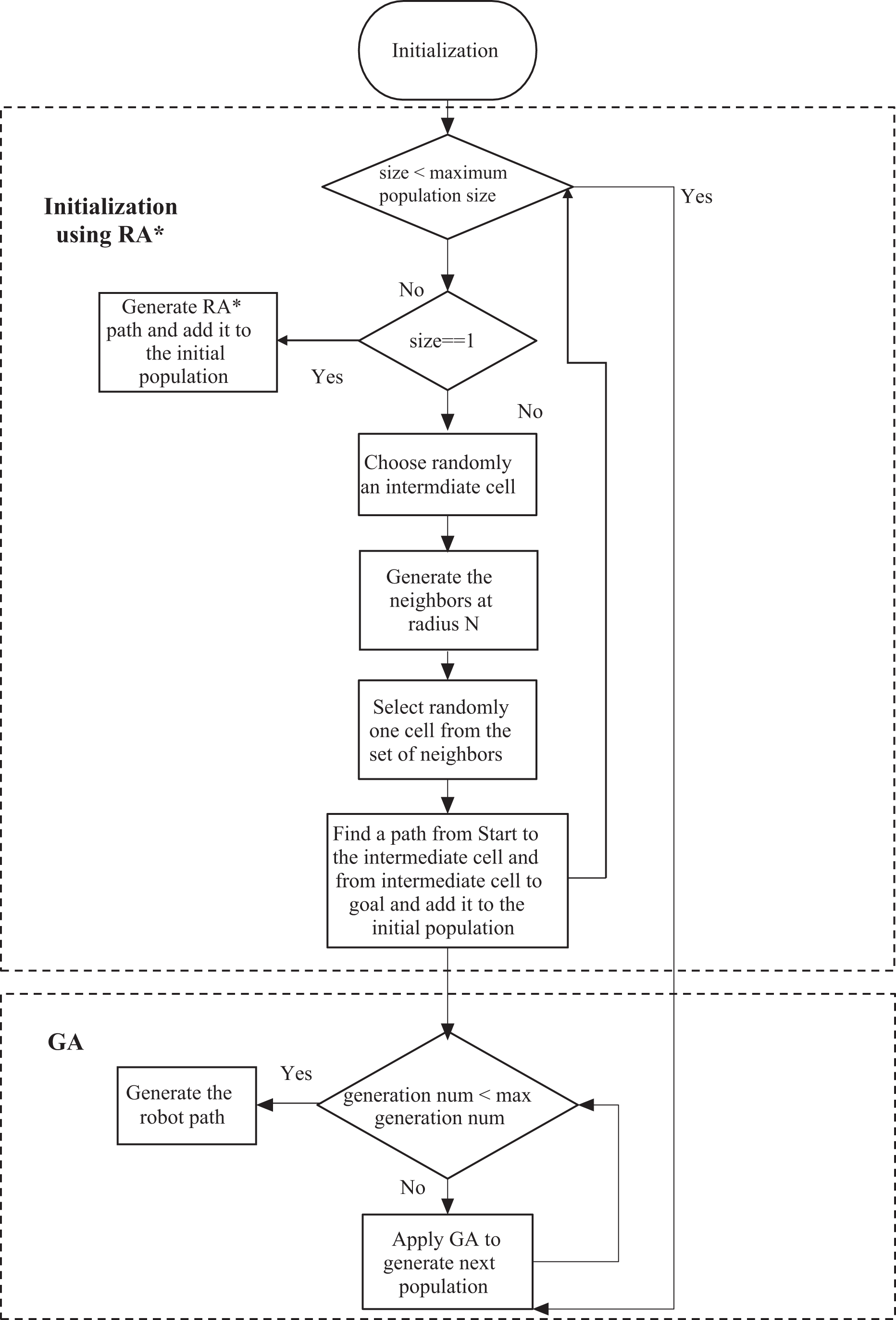
The flow chart of the RA* + GA hybrid algorithm. RA*: relaxed A-star; GA: genetic algorithm.

Algorithm 2.

The Hybrid Algorithm RA* + GA.

input : $G r i d$ , $S t a r t$ , $G o a l$

repeat

if size == 1 then

Generate the RA* path (described in Algorithm. 1)

Add the RA* to the current population.

else

Choose Randomly an intermediate cell not in

RA*.

$N e i g h b o r s_{R a d i u s N}$ : set of neighbours at Radius

N, N is a parameter.

$C r o s s_{P o i n t}$ : Select randomly one cell from

$N_{R a d i u s N}$

$P a t h_{S, C P}$ : find the path using RA* between

start cell and $C r o s s_{P o i n t}$ .

$P a t h_{C P, G}$ : find the path using RA* between

$C r o s s_{P o i n t}$ and the goal cell.

Add $P a t h_{S, C P}$ ∪ $P a t h_{C P, G}$ to the i population.

end

until (size ≥ max population size);

while (generation number < max generation number)

Use GA to generate the next population.

end

Generate the best path.

Performance evaluation

In this section, we present the simulation results of the hybrid algorithms. To evaluate the performance of the hybrid algorithms, we compared them against A* and RA*. Two performance metrics were assessed: the path length and the execution time of each algorithm. Figure 6 and Tables 5 and 6 present the average path costs and the average execution times of A*, RA*, RA*+GA and RA*+TS algorithms in different kinds of maps. Looking at these figures, we note that A* always exhibits the shortest path cost and the longest execution time. Moreover, we clearly observe that RA*+GA hybridization provides a good trade-off between the execution time and the path quality. In fact, the RA*+GA hybrid approach provides better results than RA* and reduces the execution time as compared to A* for the different types of maps. This confirms the benefits of using hybrid approaches for post-optimization purposes for large-scale environments. However, the hybrid approach using RA* and TS provides some improvements but less significant than the RA*+GA approach. In some cases, RA*+TS could not improve the RA* path cost (in video games maps and 2000 × 2000 grid maps). This can be explained by the fact that TS approach only explores the neighbourhood of the RA* solution initially generated by applying simple moves (remove, exchange, insert) which cannot significantly improve it. We can see also that all the non-optimal solutions have a small gap. Finally, the hybrid approach RA*+ACO was not successful as it does not converge easily to a better solution that the initial RA* algorithm because of the randomness nature of the ant motions and its execution time remains not interesting.

Figure 6.

Average path lengths and average execution times (log scale) of hybrid approach RA* + GA and RA* + TS as compared to A* and RA*. RA*: relaxed A-star; A*: A-star; GA: genetic algorithm; TS: tabu search.

Table 5.

Average path costs (grid units) for A*, RA*, RA* + GA and RA* + TS algorithms per environment size.

Algorithm	100 × 100	2000 × 2000	Random (512 × 512)	Rooms (512 × 512)	Video games (512 × 512)	Mazes (512 × 512)
A*	66.2	1366.4	303.4	319.1	479.5	1661.9
RA*	70.5	1443.3	319.5	350.9	493.8	1687.1
RA* + GA	68.2	1423.4	315.3	335.0	486.1	1679.2
RA* + TS	69.3	1443.3	319.5	348.2	493.8	1687.1

A*: A-star; RA*: relaxed A-star; GA: genetic algorithm; TS: tabu search.

Table 6.

Average execution times (microseconds) for A*, RA*, RA* + GA and RA* + TS per environment size.

Algorithm	100 × 100	2000 × 2000	Random (512 × 512)	Rooms (512 × 512)	Video games (512 × 512)	Mazes (512 × 512)
A*	114	296,058,499	17,626	73,438	38,649	3,161,774
RA*	17	15,414	299	724	436	5220
RA* + GA	69	59,149	1295	1813	7160	116,807
RA* + TS	110	22,258	4298	8900	16,174	51,375

A*: A-star; RA*: relaxed A-star; GA: genetic algorithm; TS: tabu search.

Integration with ROS

To demonstrate the feasibility and effectiveness of our proposed path planners in real-world scenarios, we have integrated the RA* algorithm as global path planner in the ROS³³ as possible replacement of the default navfn path planner (based on a variant of Dijkstra’s algorithm). In what follows, we present an overview of ROS, describe the integration process of RA* as global path planner and evaluate its performance against the default global path planner.

An ROS is a free and open-source robotic middleware for the large-scale development of complex robotic systems. It acts as a meta-operating system for robots as it provides hardware abstraction, low-level device control, inter-processes message-passing and package management. The main advantage of ROS is that it allows manipulating sensor data of the robot as a labelled abstract data stream, called topic, without having to deal with hardware drivers. This makes the programming of robots much easier for software developers as they do not have to deal with hardware drivers and interfaces.

Simulation model

(1) ROS navigation stack: The navigation stack³⁴ is responsible of integrating together all the autonomous navigation functions, that is, mapping, localization and path planning. To reduce the complexity of the path planning problem, the path planning task is divided into global and local planning. The move_base package is used to link the global and local planners together.

The global path planner is called before the robot starts moving to find a long-term collision free path between the start and the goal locations. The default grid-based global planner in ROS is implemented in the navfn package, and it is based on Dijkstra’s algorithm. Currently, the ROS global planner does not take into consideration the robot footprint and ignores kinematic and acceleration constraints of the robot, thus the path generated by the global planner could be dynamically infeasible.

After finishing the execution of the global planner, the local path planner (also called the controller) will be called and seeded with the global planner path to attempt following that path while considering the kinematics and dynamics of the robot besides the moving obstacle information. An ROS provides an implementation of two local planner approaches (the trajectory rollout³⁵ and the dynamic window approach³⁶) in the base_local_planner package.

(2) Integration of a new global planner to ROS navigation stack: In what follows, we present the main guidelines for integrating a new global path planner to ROS navigation stack. For more detailed step-by-step instructions, the reader is referred to our ROS tutorial available on the links in the literature.^37,38 For any global or local planner to be used with the move_base, it must first adhere to some interfaces defined in nav_core package, which contains key interfaces for the navigation stack, and then it must be added as a plugin to ROS.

All the methods defined in nav_core::BaseGlobalPlanner class must be overridden by the new global path planner. The main methods in the nav_core::BaseGlobalPlanner class are initialize and makePlan. The initialize is an initialization function that initializes the cost map for the planner. We use this function to get the cost map. The makePlan function is responsible for computing the global path. It takes the start and goal positions as an input. In this function, we first convert the start and goal coordinates into cells ID. Then, we pass those IDs with the map array to the RA* planner. To implement RA* planner, we used the sorted multiset data structure to maintain the open set, which sorted the cells based on their f_score values. This allows a significant decrease of the execution time as we only need to pick up the first element in the sorted set (having the lowest f_score) instead of searching for it in each iteration. When the planner completes its execution, it returns the computed path to the makePlan. Finally, the path will be converted to x and y coordinates and sent back to the move_base, which will publish it as a new path to ROS ecosystem.

Performance evaluation

For the experimental evaluation study using an ROS, we have used the real-world Willow Garage map, with dimensions 584 × 526 cells and a resolution 0.1 m/cell.

We considered 40 different scenarios, where each scenario is specified by the coordinates of randomly chosen start and goal cells. Each scenario, with specified start/goal cells, is repeated 30 times (i.e. 30 runs for each scenario). In total, 1200 runs for the Willow Garage map are performed in the performance evaluation study for each planner.

Two performance metrics are considered to evaluate the global planners: (1) the path length, it represents the length of the shortest global path found by the planner, (2) the execution time, it is the time spent by an algorithm to find its best (or optimal) solution.

Figure 7 shows that the RA* is faster than navfn in 82.5% of the cases. Table 7 shows that, in average, the RA* is much faster than navfn, with execution time less than 38% of that of navfn. RA* provides near-optimal paths, which are in average only 5% longer than navfn paths.

Figure 7.

Average execution time (microseconds) of RA* and navfn. RA*: relaxed A-star.

Table 7.

Execution time in (microseconds) and path length in (metres) of RA* and navfn.

Planner	Execution time		Path length
Planner	Total	Average	Total	Average
RA*	398.05	9.95 ± 0.56	941.58	23.53
navfn	643.33	16.08 ± 1.10	896.69	22.41

RA*: relaxed A-star.

Lessons learned

We have thoroughly analysed and compared five path planners for mobile robot path planning namely: A*, a relaxed version of A*, the GA, the TS algorithm and the NN algorithm. These algorithms pertain to two categories of path planning approaches: heuristic and exact methods. We also designed new hybrid algorithms and we evaluated their performance. To demonstrate the feasibility of RA* in real-world scenarios, we integrated it in the ROS and we compared it against navfn in terms of path quality and execution time. We retain the following general lessons from the performance evaluation presented in the previous sections:

Lesson 1: The study shows that heuristic algorithms are in general not appropriate for solving the path planning problem in grid environments. They are not as effective as A* since the latter always exhibits the shortest execution times and the best solution qualities. GA was found to be less effective for large problem instances. It is able to find optimal solutions like A* in some cases, but it always exhibits a greater execution time. TS was also found to be the least effective as the exploration space is very huge in large problems, and it only explores the neighbourhood of the initial solution. On the contrary, NN provides better solutions than the two aforementioned techniques.

This can be explained by two reasons: The first reason is that heuristic approaches need to generate one or several initial paths with the greedy approach (in the case of GA and TS), and this operation itself takes time which is comparable to the execution of the whole A* algorithm. The second reason is that heuristic approaches need several iterations to converge, and this number of iteration depends on the complexity of the map and the positions of the start and goal cells.

Lesson 2: The simulation study proved that exact methods in particular A* have been found not appropriate for large grid maps. A* requires a large computation time for searching path in such maps, for instance, in 2000 × 2000 grid map, the execution time of A* is around 3 h, if we fix the start cell in the leftmost and topmost cell in the grid and the goal in the bottommost and rightmost cell in the grid. Thus, we can conclude that this type of path planning approaches can be used in real time only for small problem sizes (small grid maps) or for close start and goal cells.

Lesson 3: Overall, RA* algorithm is found to be the best path planner as it provides a good trade-off of all metrics. In fact, RA* is reinforced by several mechanisms to quickly find good (optimal) solutions. For instance, RA* exploits the grid structure and approximates the g(n) function by the minimum move path. Moreover, RA* removes some unnecessary instructions used in A* which contributes in radically reducing the execution time as compared to A* without losing much in terms of path quality. It has been proved that RA* can deal with large-scale path planning problems in grid environments in reasonable time and good results are obtained for each category of maps and for different couples of start and goal positions tested; in each case, a very near-optimal solution is reached (at most 10.1% of extra length and less than 0.4% in average) which makes it overall better than A* and than heuristic methods.

The previous conclusions respond to the research question that we addressed in the iroboapp project about which method is more appropriate for solving the path planning problem. It seems from the results that heuristics methods including evolutionary computation techniques such as GA, local search techniques, namely, the TS and NNs cannot beat the A* algorithm. A* also is not appropriate to solve robot path planning problems in large grid maps as it is time consuming, which is not convenient for robotic applications in which real-time aspect is needed. RA* is the best algorithm in this study, and it outperforms A* in terms of execution time at the cost of losing optimal solution. Thus, we designed new hybrid approaches that take the benefits of both RA* and heuristic approaches in order to ameliorate the path cost without inducing extra execution time.

Lesson 4: We designed a new hybrid algorithm that combines both RA* and GA. The first phase of the RA*+GA uses RA* to generate the initial population of GA instead of the greedy approach in order to reduce the execution time, and then GA is used to improve the path quality found in the previous phase. We demonstrated through simulation that the hybridization between RA* and GA brings a lot of benefits as it gathers the best features of both approaches, which contributes in improving the solution quality as compared to RA* and reducing the search time for large-scale graph environments as compared to A*.

Footnotes

Acknowledgements

The authors would like to thank the Robotics and Internet of Things (RIoT) Unit at Prince Sultan University’s Innovation Center for their support to this work.

Declaration of conflicting interests

The author(s) declared no potential conflicts of interest with respect to the research, authorship, and/or publication of this article.

Funding

The author(s) disclosed receipt of the following financial support for the research, authorship, and/or publication of this article: This work is supported by the iroboapp project “Design and Analysis of Intelligent Algorithms for Robotic Problems and Applications” under the Grant of the National Plan for Sciences, Technology and Innovation (NPSTI), managed by the Science and Technology Unit of Al-Imam Mohammad Ibn Saud Islamic University and by King AbdulAziz Center for Science and Technology (KACST). This work is partially supported by Prince Sultan University.

References

Iroboapp: Design and analysis of intelligent algorithms for robotic problems and applications. http://www.iroboapp.org (2014, accessed 2016).

Miao

Khamis

Karray

. A novel approach to path planning for autonomous mobile robots. Int J Control Intell Syst 2011; 39(4): 1–27.

Shu

Fang

. Path planning of mobile robot in dynamic environments. In: 2011 2nd international conference on intelligent control and information processing (ICICIP), China, 25–28 July 2011, pp. 691–696. IEEE.

Randria

Khelifa

Bouchouicha

. A comparative study of six basic approaches for path planning towards an autonomous navigation. In: 33rd annual conference of the IEEE industrial electronics society (IECON), Taiwan, 5–8 November 2007, pp. 2730–2735. IEEE.

Cabreira

Dimuro

de Aguiar

. An evolutionary learning approach for robot path planning with fuzzy obstacle detection and avoidance in a multi-agent environment. In: social simulation (BWSS), 2012 third Brazilian Workshop on, Brazil, 20–23 October 2012, pp. 60–67. IEEE.

Wilensky

Evanston

. NetLogo: center for connected learning and computer based modeling. Technical Report, Northwestern University, Evanston, 1999.

Cabreira

de Aguiar

Dimuro

. An extended evolutionary learning approach for multiple robot path planning in a multi-agent environment. In: Evolutionary Computation (CEC), 2013 IEEE Congress on, Mexico, 20–23 June 2013, pp. 3363–3370. IEEE.

Hussein

Mostafa

Badrel-din

. Metaheuristic optimization approach to mobile robot path planning. In: International Conference on Engineering and Technology (ICET), Pakistan, 10–11 October 2012, pp. 1–6. IEEE.

Sariff

Buniyamin

. Comparative study of genetic algorithm and ant colony optimization algorithm performances for robot path planning in global static environments of different complexities. In: IEEE International Symposium on Computational Intelligence in Robotics and Automation (CIRA), korea, 15–18 December 2009, pp. 132–137. IEEE.

10.

Tewolde

Sheng

. Robot path integration in manufacturing processes: genetic algorithm versus ant colony optimization. In: IEEE Transactions on Systems, Man and Cybernetics, Part A: Systems and Humans, Vol. 38, 2008, pp. 278–287. IEEE.

11.

Koceski

Panov

Koceska

. A novel quad harmony search algorithm for grid-based path finding. Int J Adv Robot Syst 2014; 11(9): 144.

12.

Gomez

Santa

Sarmiento

FHM

. A comparative study of geometric path planning methods for a mobile robot: potential field and Voronoi diagrams. In: 2013 II international congress of engineering mechatronics and automation (CIIMA), Colombia, 23–25 October 2013.

13.

Cikes

Dakulovic

Petrovic

. The path planning algorithms for a mobile robot based on the occupancy grid map of the environment a comparative study. In: 2011 XXIII international symposium on information, communication and automation technologies (ICAT), Sarajevo, 27–29 October 2011.

14.

Haro

Torres

. A comparison of path planning algorithms for omni-directional robots in dynamic environments. In: IEEE 3rd Latin American robotics symposium, 2006. LARS ‘06, Santiago, 26–27 October 2006.

15.

Eraghi

Lpez-Colino

de Castro

. Path length comparison in grid maps of planning algorithms: HCTNav, a* and Dijkstra. In: 2014 IEEE conference on design of circuits and integrated circuits (DCIS), spain, 26–28 November 2014, pp. 1–6. IEEE.

16.

Pala

Eraghi

Lpez-Colino

. HCTNav: a path planning algorithm for low-cost autonomous robot navigation in indoor environments. Int J Geo-Inform 2013; 1: 729–748.

17.

Duchon

Hubinsky

Babinec

. Real-time path planning for the robot in known environment. In: 23rd international conference on robotics in Alpe-Adria-Danube region (RAAD 2014), Smolenice Castle, Slovakia, 3–5 September 2014.

18.

Chiang

Fei

JCC

. A comparative study of implementing fast marching method and A* search for mobile robot path planning in grid environment: effect of map resolution. In: IEEE workshop on advanced robotics and its social impacts, Taiwan, 9–11 December 2007, pp. 1–6. IEEE.

19.

Zaheer

Jayaraju

Gulrez

. Performance analysis of path planning techniques for autonomous mobile robots. In: IEEE international conference on electrical, computer and communication technologies (ICECCT), India, 5–7 March 2015.

20.

Al-Arif

Ferdous

Nijami

. Comparative study of different path planning algorithms: a water based rescue system. Int J Comput Appl 2012; 39: 25–29.

21.

The iPath library. 2014. https://github.com/coins-lab/ipath (accessed 2014).

22.

API documentation. http://www.iroboapp.org/ipath/api/docs/annotated.html (2014, accessed 2014).

23.

Chaari

Koubaa

Bennaceur

. On the adequacy of tabu search for global robot path planning problem in grid environments. In: 5th international conference on ambient systems, networks and technologies (ANT-2014), the 4th international conference on sustainable energy information technology (SEIT-2014), Vol. 32, Belgium, 2–5 June 2014, pp. 604–613. IEEE.

24.

Alajlan

Koubaa

Chaari

. Global path planning for mobile robots in large-scale grid environments using genetic algorithms. In: 2013 international conference on individual and collective behaviors in robotics ICBR’2013, Sousse, Tunisia, 15–17 December 2013.

25.

Chaari

Koubaa

Bennaceur

. SmartPATH: a hybrid ACO-GA algorithm for robot path planning. In: 2012 IEEE congress on evolutionary computation (CEC), Brisbane, Australia, 10–15 June 2012, pp. 1–8. IEEE.

26.

Châari

Koubâa

Trigui

. SmartPATH: an efficient hybrid ACO-GA algorithm for solving the global path planning problem of mobile robots. Int J Adv Robot Syst 2014; 11.

27.

Glasius

Komoda

Gielen

SCAM

. Neural network dynamics for path planning and obstacle avoidance. Neural Networks 1995; 8: 125–133.

28.

Hart

Nilsson

Raphael

. A formal basis for the heuristic determination of minimum cost paths. IEEE Trans Syst Sci Cybern 1968; 4: 100–107.

29.

Ammar

Bennaceur

Chaari

. Relaxed Dijkstra and A* with linear complexity for robot path planning problems in large-scale grid environments. Soft Comput J, 2015, pp. 1–23.

30.

IPath simulator. http://www.iroboapp.org/index.php?title=IPath (2014, accessed 2014).

31.

Benchmark. http://www.movingai.com/benchmarks/ (2012, accessed 2014).

32.

Grid-maps: 10 x 10 up to 2000 x 2000. http://www.iroboapp.org/index.php?title=Maps (2014, accessed 2014).

33.

Robot Operating System (ROS). http://www.ros.org (2007, accessed 2014).

34.

Marder-Eppstein

Berger

Foote

. The office marathon: robust navigation in an indoor office environment. In: Robotics and automation (ICRA), 2010 IEEE international conference, USA, 3–7 May 2010, pp. 300–307. IEEE.

35.

Gerkey

Konolige

. Planning and control in unstructured terrain. In: Workshop on path planning on costmaps, proceedings of the IEEE international conference on robotics and automation (ICRA), California, 19–23 May 2008.

36.

Fox

Burgard

Thrun

. The dynamic window approach to collision avoidance. IEEE Robot Autom Magazine 1997; 4(1): 23–33.

37.

Adding a global path planner as plugin in ROS. http://www.iroboapp.org/index.php?title=Adding_A_Global_Path_Planner_As_Plugin_in_ROS (2014, accessed 2014).

38.

Writing a global path planner as plugin in ROS. http://wiki.ros.org/navigation/Tutorials/Writing%20A%20Global%20Path%20Planner%20As%20Plugin%20in%20ROS (2014, accessed 2014).

Algorithm	100 × 100 (%)	500 × 500 (%)	1000 × 1000 (%)	2000 × 2000 (%)	Random (512 × 512; %)	Rooms (512 × 512; %)	Video games (512 × 512; %)	Mazes (512 × 512; %)
A*	100	100	100	100	100	100	100	100
RA*	5	40	60	10	5	0	20	55
GA	10	50	60	–	10	0	30	–
TS	5	0	0	–	5	0	0	–
NN	5	10	20	–	5	0	0	–

Algorithm	100 × 100 (%)	500 × 500 (%)	1000 × 1000 (%)	2000 × 2000 (%)	Random (512 × 512; %)	Rooms (512 × 512; %)	Video games (512 × 512; %)	Mazes (512 × 512; %)
A*	100	100	100	100	100	100	100	100
RA*	5	40	60	10	5	0	20	55
GA	10	50	60	–	10	0	30	–
TS	5	0	0	–	5	0	0	–
NN	5	10	20	–	5	0	0	–

Design and performance analysis of global path planning techniques for autonomous mobile robots in grid environments

Abstract

Keywords

Introduction

Motivation

Problem and solution outline

Contributions of the article

Related works

Comparative studies of heuristic and exact approaches

Comparative studies of heuristic approaches

Comparative studies of exact methods

Path planners under study

Heuristic methods

The TS algorithm

The GA

The ACO algorithm

The neural network algorithm

Exact methods

The A* algorithm

The RA* algorithm

Comparative study

Simulation environments

Simulation results

RA* + x hybrid path planners

Design of hybrid path planners

Performance evaluation

Integration with ROS

Simulation model

Performance evaluation

Lessons learned

Footnotes

Acknowledgements

Declaration of conflicting interests

Funding

References

Algorithm	100 × 100 (%)	500 × 500 (%)	1000 × 1000 (%)	2000 × 2000 (%)	Random (512 × 512; %)	Rooms (512 × 512; %)	Video games (512 × 512; %)	Mazes (512 × 512; %)
A*	100	100	100	100	100	100	100	100
RA*	5	40	60	10	5	0	20	55
GA	10	50	60	–	10	0	30	–
TS	5	0	0	–	5	0	0	–
NN	5	10	20	–	5	0	0	–