Sage Journals: Discover world-class research

Abstract

Generating smooth and continuous paths for robots with collision avoidance, which avoid sharp turns, is an important problem in the context of autonomous robot navigation. This paper presents novel smooth hypocycloidal paths (SHP) for robot motion. It is integrated with collision-free and decoupled multi-robot path planning. An SHP diffuses (i.e., moves points along segments) the points of sharp turns in the global path of the map into nodes, which are used to generate smooth hypocycloidal curves that maintain a safe clearance in relation to the obstacles. These nodes are also used as safe points of retreat to avoid collision with other robots. The novel contributions of this work are as follows: (1) The proposed work is the first use of hypocycloid geometry to produce smooth and continuous paths for robot motion. A mathematical analysis of SHP generation in various scenarios is discussed. (2) The proposed work is also the first to consider the case of smooth and collision-free path generation for a load carrying robot. (3) Traditionally, path smoothing and collision avoidance have been addressed as separate problems. This work proposes integrated and decoupled collision-free multi-robot path planning. ‵Node caching‵ is proposed to improve efficiency. A decoupled approach with local communication enables the paths of robots to be dynamically changed. (4) A novel ‵multi-robot map update‵ in case of dynamic obstacles in the map is proposed, such that robots update other robots about the positions of dynamic obstacles in the map. A timestamp feature ensures that all the robots have the most updated map. Comparison between SHP and other path smoothing techniques and experimental results in real environments confirm that SHP can generate smooth paths for robots and avoid collision with other robots through local communication.

Keywords

Path Smoothing Robot Path Planning Multi-robot Collision Avoidance

1. Introduction

Mobile robots with autonomous navigation capabilities have been used in various operations, such as industry automation, floor cleaning and managing warehouses. In these kinds of operations, multiple mobile robots are generally deployed in situations where they need to autonomously move between various locations. A smooth and continuous path is desired for robot motion that avoids abrupt and sharp turns. This problem is further complicated in the case of multiple robots as two or more robots may have intersecting and common paths, which increases the chances of a robot colliding with another robot during its operation. Hence, the path taken by each robot needs to be carefully planned. This is explained in Fig.1, where two problems need to be addressed: (1) The path of the robots must be smooth and sufficiently far from obstacles. Robot R3 in Fig.1 is dangerously close to obstacles, while the path of R4 indicates sharp turns by the robot. (2) Robots must avoid colliding with other robots that may have the same path. In Fig.1, R1 and R2 are in a deadlock position, while there is a collision possibility in relation to R4 and R5.

There is a large plethora of research literature on path planning for autonomous robots. Back in 1960, Pollock and Wiebenson [1] first reviewed various algorithms to find a minimum cost path from any given graph. Another influential prior work by Peter Hart et al.[2], from 1968, incorporated heuristic information into graph searching to find minimum cost paths. In 1979, Thomas et al. proposed an algorithm[3] for collision-free paths in an environment with polyhedral obstacles. Since then, a number of path planning algorithms has been proposed; a detailed summary of these algorithms can be found in [4, 5] and [6]. Among these, the $A *$ algorithm [2], the D* algorithm [7, 8], the probabilistic roadmap planner (PRM) [9], the rapidly-exploring random tree (RRT) [10, 11] and potential fields algorithms [12] are the most widely used techniques today.

In general, path planning is carried out in global and local planning. First, it is necessary to find the overall path from the start until the goal location that avoids the static obstacles in the map. This is undertaken during global planning. At this stage, it is neither necessary to consider the dynamic obstacles of the environment, nor worry about the fine control sequences that need to be sent to the robot to take the turns. Dijkstra‵s uniform-cost search algorithm[13] has widely been used for global planning. However, it is computationally expensive with a time complexity of $O (N^{2})$ , where N is the number of nodes. A number of ways to optimize the algorithm[14] and its variants[15] has been proposed. The A* algorithm [2] is an extension of Dijkstra‵s algorithm with better time performance including a good initial heuristic. The D* (or Dynamic A*), which finds an optimal path in real time by incrementally updating paths to the robot‵s state as new information is discovered, is more efficient than the A* algorithm. The RRT algorithm [10, 11] efficiently searches high-dimensional spaces by building space-filling trees randomly. The RRT algorithm plans a path with a biased growth towards the goal with high probability. A review of many variations and implementations of RRT planners has been undertaken by S. LaValle et al. in [16].

Figure 1.

Two problems faced by multi-robot path planning: (1) the paths should be short, smooth and safe (i.e., far from obstacles); (2) robots must avoid colliding with each other

The next step is that of local planning, which focuses on generating smooth curves along the global path. Where sharp and angular turns on the paths are sometimes infeasible and difficult for robot control, this situation needs to be smoothed out, such that the robot can move continuously and avoid abrupt motion. Path smoothing using parametric curves was proposed as early as 1957 by L. Dublin in [17, 18]. Generally known as Dublin curves, they employ lines and circles, but suffer from the problem of discontinuities. Since then, path smoothing using various types of curves has been proposed. Those worth mentioning are proposals that make use of clothoids [19, 20], quintic G² splines [21] and intrinsic splines [22]. Other approaches includes curves with closed-form expressions such as the B-spline [23], quintic polynomials [24] and the Bezier curve [25]. However, as these methods suffer from problems of complicated curvature functions with many parameters, improved methods have been proposed [26]. There is a different, but old, class of path smoothing algorithms that employ interpolation [27]. Interpolation techniques were proposed as early as 1779 by E. Warning in [28] (an English translation of the original German work is available at [29]). These techniques are generally plagued by computational costs and Runge‵s phenomenon [30], which is a classic illustration of polynomial interpolation non-convergence. Recently, a very inspiring work ([31] and [32]) by S. R. Chang and U. Y. Huh proposed a quadratic polynomial and membership interpolation (QPMI) algorithm, which avoids Runge‵s phenomenon [30] and the weakness of spline interpolation, by creating a G² continuous path using just the quadratic polynomials and membership functions. In [32], they propose a collision-free continuous G² path using interpolation. However, their methods require explicit collision detection checks, and reprogramming of smooth paths, which can be expensive in the case of crowded environments. [33] provides a useful resource that summarizes various path smoothing techniques.

The discussion of the aforementioned algorithms refers to the state of the art regarding path planning for a single robot. We now briefly discuss the previous situation regarding multi-robot collision-free path planning. In a broad sense, multi-robot planning algorithms may be either coupled, in which the paths of all the robots are calculated concurrently, as in [34], or decoupled [35], in which the path of each robot is individually calculated, while the velocities are later tuned to avoid collision, as in [36]. Many prior works address smooth path generation and multi-robot collision-free path planning as separate problems. For example, the work by Yang et al. [37] proposes to use polygons around the crossing points of skeleton maps. However, their method produces a path with many sharp turns, which is undesirable for robot motion. We believe that smooth path generation and multi-robot collision avoidance are integrated problems and must be addressed together. In other words, robots must traverse smooth paths while they are avoiding collision with other robots.

This paper proposes SHP to produce smooth paths for robot motion using the geometry of hypocycloids [38, 39]. SHP fall into the later category of local planning to generate smooth paths. Smooth paths avoid sharp and angular turns, as well as keep the robot at a safer distance from the environmental obstacles. We define diffusion as moving a point along the segment(s). An SHP works by diffusing the intersecting points of skeleton maps[40], which are generated by thinning [41] or Voronoi diagrams [42] into nodes, thereby generating continuous hypocycloidal curves using the diffused nodes. Well-known path planning techniques, such as the $A *$ algorithm [2] and the D* algorithm [7, 8], are used to generate the global motion policy, after which SHP smooths out the sharp turns. A decoupled multi-robot scheme involving SHP is also proposed, in which the diffused nodes are used as retreat points for the robot to avoid collision with other robots.

The novel contributions of the paper are:

The proposed SHP is the first use of hypocycloidal geometry to generate smooth continuous paths for robot motion. A mathematical derivation of SHP is presented in Section 3.

To the best of our knowledge, the proposed work is also the first to consider the case of a smooth path traversal that maintains a safe clearance distance from the obstacles involving a load carrying robot (where the load is both centred and uncentred). This is important because the collision-free smooth path traversed by a robot will be different, depending on whether it is carrying or not carrying a load. Section 4 explains the calculation of the clearance threshold distance in both cases in mathematical terms.

A decoupled collision-free multi-robot path planning integrated with SHP is proposed (Section 5). It is advantageous as the robot still traverses smooth paths, while also avoiding collision with other robots. Intelligent communication between robots is important in a decoupled multi-robot path planning scheme. This work proposes the novel and practical idea of ‵node caching‵ for better efficiency (Section 5.1).

An integrated dynamic obstacle avoidance involving SHP with a ‵map update‵ is proposed. The robot finds a new SHP path if a dynamic obstacle is encountered and shares the coordinates of the dynamic obstacle with other robots. Only the coordinates are transferred for efficiency. This is explained in Section 6.

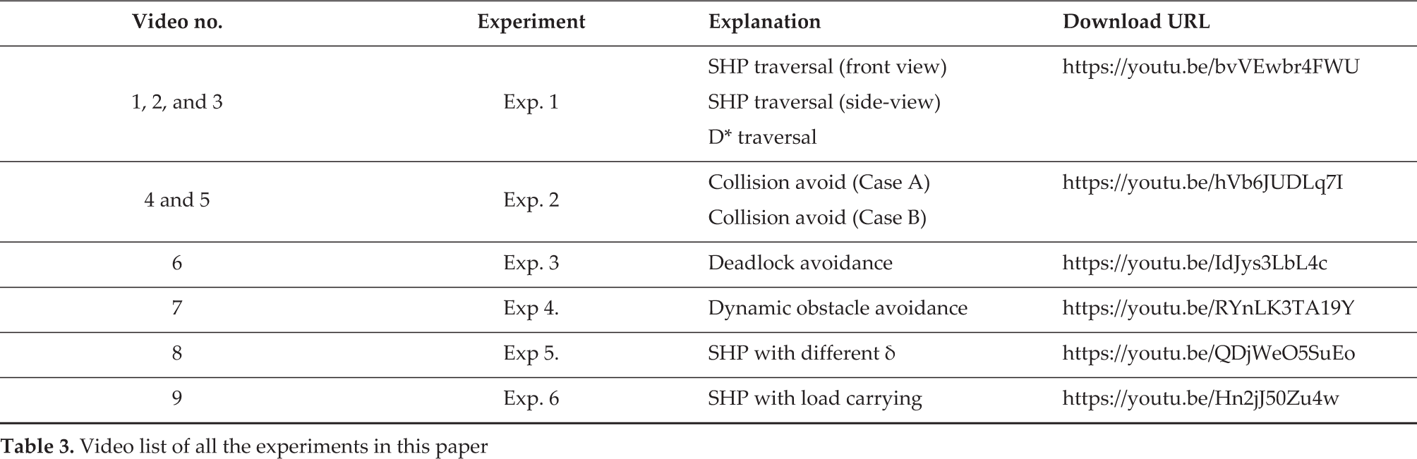
Experiments (Section 9) in real environments with robots were performed to test the proposed techniques. We have also compared (Section 11) the performance of the proposed SHP with standard path planning techniques, such as the D*[7, 8], the PRM[9] and the recently proposed QPMI[31] algorithm based on a G² collision-free smooth path[32]. In so doing, we found that SHP give a better performance without explicit collision detection, while maintaining safe clearance in relation to the obstacles, even when a load is carried. Furthermore, readers are strongly encouraged to refer to all the experimental videos that have been provided online, whose URLs are summarized in Table 3, in the course of reading this manuscript.

2. Skeleton Map and Node Generation

We first briefly discuss skeleton maps and nodes or points of intersection in these maps, which need to be generated from a map constructed by a robot using exteroceptive sensors. A grid map is generated using sensors, such as laser range or RGBD sensors, which are attached to the robot. For noisy environments, mapping techniques proposed in [43, 44] can be used. Later, we apply mathematical morphological operations [45, 46] to produce dilation, followed by erosion to remove noise, which may appear in the map as small dots from the laser range sensor. To remove larger blobs, dilation can be carried out multiple (three to four) times followed by a single erode. A Voronoi map generated from the binary map has the path [42], which keeps the robot at a safe distance from obstacles, but also has sharp turns, as shown in Fig.3(c), in which the robot encounters sharp turns at O from L_C or L_A to L_B. Similarly, a skeleton path[40] that is generated, for example, by the thinning technique [41], as in the case of Fig 4(a), will resemble the shape of the English alphabet T, whose cross-point is shown at O. However, most thinning algorithms do not generate a sharp point with perpendicular turns, such as point ‵o‵ shown in Fig 4(a); rather, they generate three points close to each other. To generate a single point, we use a modification of the thinning algorithm proposed by T. Zhang et al. [47]. After generating the skeleton map by thinning, turn points are detected on the path. Later, the points that are close to each other are clustered to generate a single point called a node. This is shown in Fig.2(b), which represents the skeleton map of Fig.2(a). The enlarged portion in Fig.2(b) shows the three points where turns occur on the pathway in red, while a single cluster is shown in blue. Thinning algorithms suffer from the problem of generating too many undesirable sub-branches, which can be removed by pruning algorithms[48].

These nodes along the Voronoi or skeleton paths will be used to generate the SHP discussed in the next section.

3. Generating SHP

A hypocycloid is a geometrical curve that is produced by a fixed point P, which lies on the circumference of a small circle of radius r_s rolling inside a larger circle of radius $R_{L} > r_{s}$ [38, 39]. As shown in Fig.3, the rolling circle has a radius of r_s and the large circle has a radius of R_L, while the curve is defined in general by the following:

\begin{array}{l} x (θ) = (R_{L} - r_{s}) \cos (θ) + r_{s} \cdot \cos (\frac{R_{L} - r_{s}}{r_{s}}) θ \\ y (θ) = (R_{L} - r_{s}) \sin (θ) + r_{s} \cdot \sin (\frac{R_{L} - r_{s}}{r_{s}}) θ \\ or, x (θ) = R_{L} \cdot ξ {(η - 1) \cos (θ) + \cos ((η - 1) θ)} \\ y (θ) = R_{L} \cdot ξ {(η - 1) \sin (θ) + \sin ((η - 1) θ)} \end{array}

(1)

where η is the number of cusps and ξ is the ratio of the radius of the rolling circle in relation to the radius of the large circle, i.e., $ξ = \frac{r_{s}}{R_{L}}$ . A cusp is defined as the sharp corner where the curve is not differentiable. Fig.3(a) shows a three-cusped hypocycloid, which is referred to as a deltoid or a tricuspoid. An astroid is a four-cusped hypocycloid, as shown in Fig.3(b).

Figure 2.

Node extraction from a skeleton map: (a) a map with obstacles and free space; (b) a corresponding skeleton map. Nearby nodes are clustered to form a single node.

Figure 3.

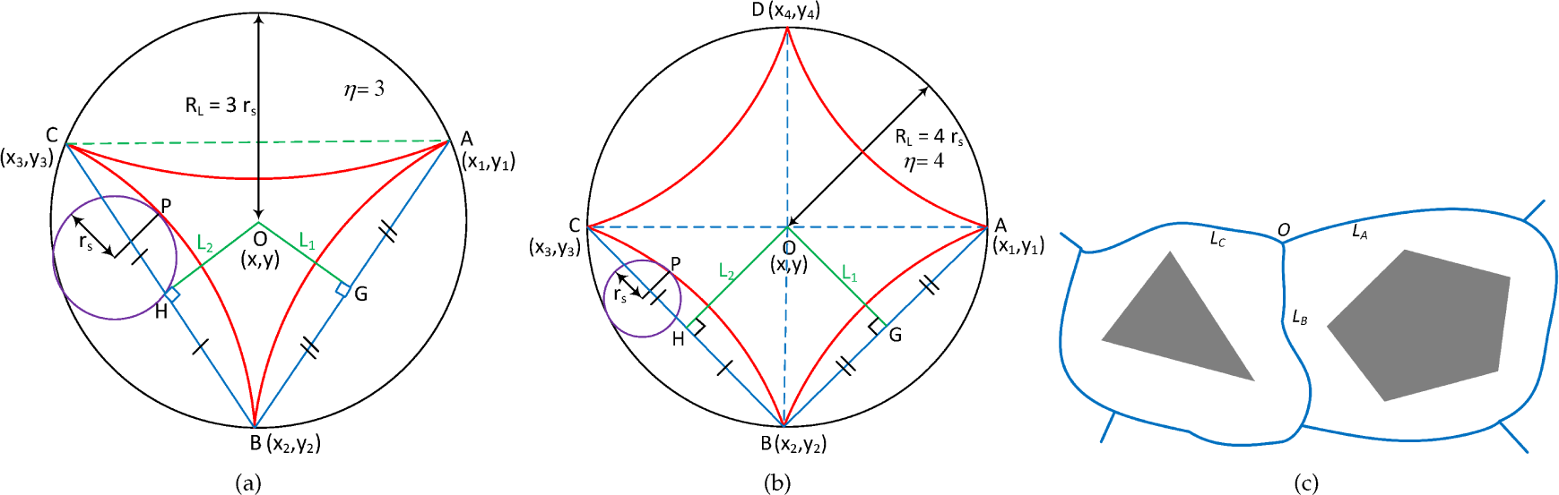
Geometry of hypocycloid curves, as shown in red: (a) deltoid curve - $R_{L} = 3 \times r_{s}, ξ = \frac{1}{3}$ ; (b) astroid curve - $R_{L} = 4 \times r_{s}, ξ = \frac{1}{4}$ ; and (c) Voronoi paths, which keep a safe distance from obstacles, although the robot encounters sharp turns at O from L_C or L_A to L_B

Figure 4.

Smooth path generation with: (a) a deltoid or the lower half of an astroid curve; (b) astroid curves in the crossroad map; (c) a portion of a hypocycloid to generate a curve at the corner

In general, to obtain n cusps in a hypocycloid, the radius of the smaller circle is set to $r_{s} = \frac{R_{L}}{n}$ , given that n rotations of the smaller circle bring it back to the original position, generating n cusps during the traversal [38]. For a deltoid, $R_{L} = 3 \times r_{s}, ξ = \frac{1}{3}$ , whereas, for an astroid, $R_{L} = 4 \times r_{s}$ and $ξ = \frac{1}{4}$ .

As shown in Fig 4(a), a robot moving from location L_C to location L_B will encounter a very sharp turn of nearly 90 degrees at point o along path $C o B$ . The same is true for path $A o B$ . To avoid sharp turns, we diffuse the node o along the open path directions of $\vec{o A}, \vec{o B}$ and $\vec{o C}$ . This diffusion is continued until the magnitude of the vectors (i.e., $| \vec{o A} |$ , $| \vec{o B} |$ and $| \vec{o C} |$ ) are such that the line segment $\bar{B C}$ and $\bar{A C}$ are far from the surrounding obstacle by obstacle clearance distance δ. The value of clearance distance δ is precalculated and will depend upon the geometry and dimension of the robot, as well as the obstacle. Now, a robot moving from location L_C to location L_B can avoid making a sharp turn at point o by taking a right turn at point C, traversing the path $C B$ , shown as a blue line in Fig 4(a), then taking a right turn again at point B and continuing straight to location L_B. However, we find that the robot still has to make a considerably sharp turn (shown by $∠ α_{i}$ ) at points A, B and C, which is not desirable.

We further improve the smoothness of the path by applying hypocycloidal geometry and generating curves $\overset{⌢}{A B}$ and $\overset{⌢}{B C}$ , which are shown in red in Fig.4(a). The mathematical derivation of generating hypocycloidal curves is also presented.

An explanation using the previous case shown in Fig.4(a) is provided. Let $(x_{1}, y_{1})$ , $(x_{2}, y_{2})$ and $(x_{3}, y_{3})$ be the coordinates of points A, B and C, respectively. If d_c represents the distance between the left obstacle and line segment $\bar{B C}$ and the right obstacle and $\bar{A B}$ , then diffusion is performed incrementally in very small steps of d_c. The coordinates of points $A, B,$ and C will be known once the diffusion of point o stops at the stage when condition $d_{c} = δ$ is satisfied. Although the value of δ may be different for different obstacles ( $δ_{i} \neq δ_{j}, i \neq j$ ), we assume, for the sake of simplicity, that the clearance distance is the same. The case of different clearance distances is discussed later.

We generate a hypocycloid (astroid) curve with points A, B and C. Points A, B and C in Fig.4(a) correspond to respective points in Fig.3(b). In Fig.3(b), the midpoints of line segments $A B$ and $B C$ are $G (\frac{x 1 + x 2}{2}, \frac{y 1 + y 2}{2})$ and $H (\frac{x 2 + x 3}{2}, \frac{y 2 + y 3}{2})$ , respectively. The slope of line $\bar{A B} (m_{1})$ is $\frac{y 2 - y 1}{x 2 - x 1}$ and the slope of line $\bar{B C} (m_{2})$ is $\frac{y 3 - y 2}{x 3 - x 2}$ . Hence, the slope of lines L₁ and L₂, which are perpendicular to $\bar{A B}$ and $\bar{B C}$ , are $\frac{- 1}{m 1}$ and $\frac{- 1}{m 2}$ , respectively. Hence, the equation of line L₁ is:

\begin{array}{l} y - \frac{y 1 + y 2}{2} = - \frac{1}{m_{1}} (x - \frac{x 1 + x 2}{2}) \\ or, y_{1 p} = - \frac{1}{m_{1}} (x - \frac{x 1 + x 2}{2}) + \frac{y 1 + y 2}{2} \end{array}

(2)

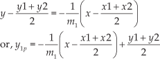
For L₂, it is:

\begin{array}{l} y - \frac{y 2 + y 3}{2} = - \frac{1}{m_{2}} (x - \frac{x 2 + x 3}{2}) \\ or, y_{2 p} = - \frac{1}{m_{2}} (x - \frac{x 2 + x 3}{2}) + \frac{y 2 + y 3}{2} . \end{array}

(3)

Lines L₁ and L₂ intersect at the centre of the circle O ( $∴ y_{1 p} = y_{2 p}$ ). From Eq.2 and Eq.3:

\begin{array}{l} - \frac{1}{m_{1}} (x - \frac{x 1 + x 2}{2}) + \frac{y 1 + y 2}{2} = \\ - \frac{1}{m_{2}} (x - \frac{x 2 + x 3}{2}) + \frac{y 2 + y 3}{2} \\ or, - \frac{x}{m_{1}} + \frac{x 1 + x 2}{2 m_{1}} + \frac{y 1 + y 2}{2} = \\ - \frac{x}{m_{2}} + \frac{x 2 + x 3}{2 m_{2}} + \frac{y 2 + y 3}{2} . \end{array}

(4)

After solving Eq. 4, we get the centre of the circle O ( $O_{x}, O_{y}$ ) and radius R_L as follows:

\begin{array}{l} O_{x} & = - \frac{m_{1} m_{2} (y 3 - y 1) + m_{1} (x 2 + x 3) - m 2 (x 1 + x 2)}{2 (m_{1} - m_{2})} \\ O_{y} & = \\ = - \frac{1}{m_{1}} (- \frac{m_{1} m_{2} (y 3 - y 1) + m_{1} (x 2 + x 3) - m 2 (x 1 + x 2)}{2 (m_{1} - m_{2})} \\ - \frac{x 1 + x 2}{2}) + \frac{y 1 + y 2}{2} \\ R_{L} = \sqrt{{(x_{i} - O_{x})}^{2} + {(y_{i} - O_{y})}^{2}}, i \in 1,2 or 3. \end{array}

(5)

Figure 5.

Smooth path generation when clearance thresholds are not same: (a) & (b) a lower astroid with $δ_{1} \neq δ_{2}$ ; the dotted lines and points $A^{'}$ and $B^{'}$ are auxiliary

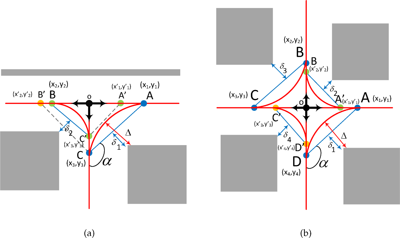
Once the radius of the larger circle R_L is found, the value of the radius of smaller rolling circle r_s can also be found. In the case of an astroid, $r_{s} = \frac{R_{L}}{4}$ . Curves $\overset{⌢}{A B}$ and $\overset{⌢}{B C}$ , which are shown in red in Fig.4(a), can now be found easily from Eq. 1.

In the case of Fig.4(b) as well, a smooth path can be obtained from the geometry of an astroid. The steps for curve generation are similar to those described above. As shown in Fig.4(b), any traversal with a turn across the point o would encounter a sharp turn. Even in the case where the paths cross the blue lines, which represent line segments $\bar{A B}$ , $\bar{B C}$ , $\bar{C D}$ or $\bar{D A}$ , the robot has to attempt sharp turns. However, a smooth path is generated along the astroid curves $\overset{⌢}{A B}$ , $\overset{⌢}{B C}$ , $\overset{⌢}{C D}$ and $\overset{⌢}{D A}$ , as shown in red.

For the corner section of the map, a section of an astroid or a deltoid can be used for smooth path generation. For example, in the case of Fig.4(c), which represents a corner section, only a section of an astroid across curve $\overset{⌢}{A B}$ is used (other curves are omitted). Notice that, in the case of Fig.4(a), the curves $\overset{⌢}{A B}$ and $\overset{⌢}{B C}$ were also generated from an astroid by using the two lower curves, while omitting the upper curves.

We now consider the case in which the clearance thresholds for different obstacles are not equal, i.e., $δ_{i} \neq δ_{j}, i \neq j$ . Although a maximum unique value of clearance threshold $δ_{m a x}$ is desired, the value may vary in situations where parts of the map are too narrow and $δ_{m a x}$ clearance is not possible, such that the actual clearance value is smaller than $δ_{m a x}$ . This kind of situation is described in Fig.5(a) and Fig.5(b). A simple and straightforward solution could be to obtain the minimum of $δ_{i}, i \in {1,2, \dots, n}$ and generate curves using the $δ_{m i n}$ . However, this would be inefficient, as some paths would have lesser clearance in situations where more clearance was possible. In Fig.5(a), the clearance equates to $δ_{1} \neq δ_{2}$ , while the obstacle on the left side is slightly higher up compared with the one on the right side. In this case, each curve is individually formed when taking individual clearance threshold into consideration. For the curve $\overset{⌢}{B C'}$ , point $A^{'}$ is assumed and curve $\overset{⌢}{B C'}$ is generated using only δ₂ clearance as well as points $A^{'}$ , B and $C^{'}$ . Similarly, point $B^{'}$ is assumed and curve $\overset{⌢}{A C}$ is generated with δ₁ clearance along with points A, $B^{'}$ and C. Even though the line $\bar{B^{'} C}$ is closer to the obstacle, while clearance δ₂ is not obeyed, this is permitted given that the curve $\overset{⌢}{B' C}$ is auxiliary and will not be a part of the actual path. The final and actual paths generated have curves $\overset{⌢}{A C}$ and $\overset{⌢}{B C'}$ , along with line $\bar{A B}$ . Similarly, in Fig.5(b), curves are individually generated for each clearance δ_i.

In all cases, it can geometrically be shown that the new obstacle clearance is defined by $Δ_{i} > δ_{i}$ , as shown in Fig.4(a), 4(b), 4(c), 5(a) and 5(b). Hence, the path is not only smooth, but also safe and avoids collision with environmental obstacles. Each of the points ( $A, B, C, D$ ) formed after diffusion is referred to as a node.

Figure 6.

SHP generation with different angles. The first segment of the curve in blue is taken to generate SHP, whereas other curve segments in black and red are ignored. The red curve segment shows the portion of the hypocycloid that fails to close on the start point because the angle does not perfectly divide into 360 degrees. (a) $θ = 15.3$ ; (b) $θ = 31.4$ ; (c) $θ = 64$ ; (d) $θ = 78$ ; (e) $θ = 111.9$ ; (f) $θ = 150$ .

Figure 7.

Applying transition curves for smoothing joints between straight segments and curves: (a) a transition curve (blue) gradually decreasing curvature from infinity (online) to that of an SHP (red); (b) employing transition curves with SHP in an environment in which a smooth path is obtained, as shown in red

3.1. SHP for different angles

Skeleton maps can generate paths in which segments make different angles that are not necessarily 90 degrees. SHP can generate smooth paths for all angles. For any angle θ, the total number of cusps is given by $\frac{360}{θ}$ (θ in degrees). If $\frac{360}{θ}$ is a whole number, then the hypocycloid curve closes in on itself, as in the case of an astroid ( $θ = 90$ degrees). If $\frac{360}{θ}$ is a fraction, then the curve does not closes in on itself. However, irrespective of whether the hypocycloid closes in on itself or not, we simply take the first hypocycloid curve segment generated and discard the rest of the curve segments. SHP curves for different angles are shown in Fig.6. In all cases relating to Fig.6, the first blue curve segment is taken to generate SHP, whereas other segments are ignored. In all cases, the red curve is the last curve segment that fails to close at the starting point of the hypocycloid. It is also discarded.

First, the angle between the two line segments ( $θ_{m a x}$ ) is calculated from any two points, i.e., ( $x_{1}, y_{1}$ ) and ( $x_{3}, y_{3}$ ), on respective line segments and the intersection point or the node ( $x_{2}, y_{2}$ ). These three points form a triangle. According to the cosine rule, we find the angle $θ_{m a x}$ as follows:

\begin{array}{l} θ_{m a x} = {cos}^{- 1} (\frac{a^{2} + c^{2} - b^{2}}{2 a c}), \\ where, \\ a = \sqrt{{(x_{3} - x_{2})}^{2} + {(y_{3} - y_{2})}^{2}}, \\ b = \sqrt{{(x_{3} - x_{1})}^{2} + {(y_{3} - y_{1})}^{2}}, \\ c = \sqrt{{(x_{1} - x_{2})}^{2} + {(y_{1} - y_{2})}^{2}} . \end{array}

(6)

The first segment of the SHP curve is generated using the parametric equation given by Eq.1, which sets the parameter η (number of cusps) to $\frac{360}{θ_{m a x}}$ (e.g., for an astroid, $θ_{m a x} = 90$ , hence $η = 4$ ; for $θ_{m a x} = 131.94$ , $η = 2.728$ ). The value of θ is then varied from 0 to $\frac{θ_{m a x} π}{180}$ in small increments of θ (e.g., 0.01, depending upon the density of the points desired in relation to an SHP with smaller increments producing denser points). Since we started the value of the angle θ from zero, the coordinate system employed in turn needs to be transformed to the local coordinates.

3.2. SHP curvature and continuity

SHP curvature is generated using parametric equations described in Eq. 1 for a given clearance distance. If φ is the angle from the centre of the larger circle to that of the smaller circle, then curvature $c (φ)$ is defined as [39],

\begin{array}{l} c (ϕ) = \frac{2 R_{L} - r_{s}}{4 r_{s} (R_{L} - r_{s})} cosec (\frac{a ϕ}{2 r_{s}}) . \end{array}

(7)

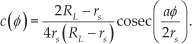
Arc length ( $s (φ)$ ) can then be found by integrating the differential displacement $d l$ over the curve γ as follows:

\begin{array}{l} s (ϕ) & =_{\int}^{γ} | d l | \\ = \frac{8 (R_{L} - r s) r_{s}}{R_{L}} {sin}^{2} (\frac{R_{L} ϕ}{4 r_{s}}), \end{array}

(8)

Meanwhile, the tangential angle is as follows:

\begin{array}{l} ϕ_{θ} (ϕ) = (1 - \frac{R_{L}}{2 r_{s}}) ϕ . \end{array}

(9)

From Eq.(7), the curvature of a hypocycloid gradually decreases to a minimum value, then gradually increases again to meet a point on the straight segment, which makes SHP ideal for curve generation between two points on the segments of skeleton paths. Compare this to a clothoid [49], whose curvature is equal to its arc length which, in turn, is equal to the parameter θ. This property makes clothoids a good choice for global smoothing of curves [19, 20]. However, as θ increases, clothoids degenerate quickly and are difficult to fit between points on the skeleton paths. Moreover, unlike hypocycloids, clothoids are generally defined by Fresnel integrals[50], which are transcendental functions and, unlike algebraic functions, do not satisfy a polynomial equation. In the case of robots with an on-board computer, these are expensive to compute compared to hypocycloids, which can be computed fast. This could also be a critical factor in the real-time manoeuvre of a robot in avoiding obstacles while traversing a newly computed smooth path.

The continuity of the curves is often discussed geometrically. A $G 0$ continuous path connects all the points between the start and the goal location, such that there is no gap. A $G 1$ continuous path also preserves the tangency between the points. In other words, the path first matches differential values at each point in the path. A $G 2$ continuous path preserves the second differential values at each point in the path. In general, a curve has $C^{n}$ continuity if its $n^{t h}$ derivative $\frac{d^{n} s}{d t^{n}}$ is also continuous. In terms of robot motion, the $G 1$ continuous motion preserves velocity, whereas the $G 2$ continuous path preserves acceleration.

Many previously proposed path smoothing techniques [32, 31, 51, 52] attempt to smooth out the global path, for example, by interpolating global points (calculated by PRM or other techniques) from start to goal. This approach preserves the geometric continuities. However, most of these points also lie on straight passages, while the path unnecessarily ends up in a wavy form and comes close to one of the walls of the corridors. The global path smoothing techniques proposed in these works are quite interesting. However, most of these works assume the robot to be a point entity, while issues such as topological admissibility are completely ignored. Particularly in the case of narrow passages, they generate paths that are dangerously close to walls and undesired for robot motion. This is discussed in detail in Section 11.

In this paper, SHP are introduced as local path smoothers, not global ones. In other words, in all the aforementioned examples, only the turns in the skeleton path were smoothed out, whereas the already existing straight line segments of the skeleton map were untouched. This is desirable because, if we consider a straight corridor, a robot is expected to move on a straight path, keeping equal distance from the walls on both sides.

SHP preserve $G 1$ continuity, while SHP segments are tangential to the straight segments. However, $G 2$ continuity is not guaranteed. This is not a problem within the bounds of the robot travelling at low speed (as also experimentally verified by the results in Section 9). In the case of robots travelling with high speed, in which there is acceleration relating to SHP, $G 2$ continuity is desired, whereas the transition between the straight line and the curved section can be further smoothed out, even though it is sufficient for most practical cases involving indoor robots moving at low speeds. This is a well- studied problem and various solutions are available. In fact, smoothing out a straight section of track to a curved section, while maintaining curvature continuity using transition curves [53], has extensively been studied for building railway tracks and road highways. We briefly discuss transition curves, as their solutions in parametric forms can easily be obtained and computed.

Transition curves [53] connect a straight segment of the path at one end with the curve at the other end. Hence, the radius of curvature changes from zero on the straight segment to a finite value of the curve, at a uniform rate. It eliminates the kink generated by directly connecting the straight and the curved section. Transition curves have the following important properties desirable for robot motion: (a) they are tangential to the straight line of the path, i.e., the curvature at the start is zero; (b) they join the circular curve tangentially; and (c) their curvature increases at the same rate. Transition curves have rigorously been studied for G2 continuity in many works [54, 55, 56], and can also provide smooth G2 transition between two straight lines.

Fig. 7(a) shows a curved path in red, which meets the straight segment at point A. To generate the transition curve, point A is shifted back to A′, which is the starting point of the transition curve shown in blue. Although different types of curves can be used to generate transition curves, Euler‵s curves are the most common[53]. Taking into account the linear increase of the curvature from zero on the straight segment to the curvature of the hypocycloid, the rate of change of the angle at any point (P) on the transition curve of length L (shown in blue in Fig.7(a)) is given by:

\begin{array}{l} \frac{d θ}{d s} = \frac{s}{R_{L} \cdot L}, \end{array}

(10)

where s is the length of the transition curve from point A′ to P in Fig.7(a). Integrating Eq.10, we obtain:

\begin{array}{l} θ = \frac{s^{2}}{2 R_{L} \cdot L} . \end{array}

(11)

During the initial condition (on the straight segment) when $s = 0$ , θ is also 0. Apart from polar coordinates, the equation of the transition curve in parametric form is given as[53, 57]:

\begin{array}{l} x & = s - \frac{s^{5}}{40 R_{L}^{2} L^{2}}, \\ y & = \frac{s^{3}}{6 R_{L}} - \frac{s^{7}}{336 R_{L}^{3} L^{3}} . \end{array}

(12)

Fig.7(b) shows SHP results with transition curves from point P to Q. In Fig.7(b), $∠ A O B = 120$ , such that a deltoid curve is used. Similarly, $∠ C O^{'} D = 64$ and a six-cusped hypocycloid is used. Initial points of contact A, B, C and D have been shifted to A′, B′, C′ and O′, respectively. The amount of shift is determined experimentally and larger for smaller values of $θ_{m a x}$ , and vice versa. In order to minimize this shifting, the SHP curve itself gets slightly shifted downwards[53], although it is a good approximation of the original curve. Moreover, it is not computationally expensive to generate transition curves, which can easily be computed from the parametric equation (Eq.12).

Figure 8.

Determining clearance threshold δ in the case of a load carrying robot: (a) no load; (b) centred load; (c) uncentred load (robot turning right); (d) uncentred load (robot turning left)

4. Determining Clearance Distance (δ)

Many path planning techniques ignore the practical case of a mobile robot carrying load. However, this is important and we discuss both the cases to calculate the value of the threshold clearance distance δ when the robot is not carrying any load, as well as when the robot is carrying some load. Since the sensors mounted on the robot are prone to errors, the robot motion is uncertain, such that the clearance threshold is increased by an additional distance $δ_{b u f}$ . Clearance threshold $δ_{N L}$ in the case of no load is given as:

\begin{array}{l} δ_{N L} = \frac{W}{2} + δ_{b u f}, \end{array}

(13)

where W is the width of the robot. Fig.8(a) shows the case of a robot that carries no load. The clearance threshold (δ_L) in the case of a load carrying robot is given as:

\begin{array}{l} δ_{L} = \frac{W_{e f f}}{2} + δ_{b u f}, \end{array}

(14)

where the effective width ( $W_{e f f}$ ) of the robot needs to be calculated for the following three cases:

Small load: This implies the case when the load (of length L) is small enough to be within the frame of the robot, i.e., $L < W$ . This case is considered to be similar to a robot not carrying any load and $δ_{L} = δ_{N L}$ .

Centred load: This implies the case when the load is centred on the robot. In other words, a load of length L has dimensions $\frac{L}{2}$ on either side of the centre point of the robot. Fig.8(b) depicts such a situation. The effective width of the robot is equal to half of the load length (i.e., $W_{e f f} = \frac{L}{2}$ ).

Uncentred load: This implies the case when the load is not centred on the robot. In other words, a load of length L has dimensions greater than $\frac{L}{2}$ on any of the sides from the centre point of the robot. This situation is depicted in Fig.8(c) and Fig.8(d). Notice that the effective width of the robot ought to change according to the direction of motion of the robot and the position of the obstacle, which is the total load length hanging out from the centre of the robot frame. In the case of Fig.8(c), load length is more on the right side of the robot, as is the obstacle. Hence, the effective robot width $W_{e f f} = | \vec{L_{d i r}} | + \frac{W}{2}$ , where $| \vec{L_{d i r}} | = | \vec{L_{R}} |$ represents the load length on the right side of robot frame. In the case of Fig.8(d), the robot obstacle is on the left hand side of the robot, while the load length on the left side is smaller than the right side (i.e., $| \vec{L_{L}} | < | \vec{L_{R}} |$ ). The effective width of the robot is also smaller from the point of view of the obstacle in this case.

Simply put, the effective width is given by:

W_{e f f} = (\begin{matrix} \frac{W}{2} & W \geq L Centred Load \\ \frac{L}{2} & L > W Centred Load \\ \frac{W}{2} + | \vec{L_{d i r}} | & L > W Uncentred Load \end{matrix}

(15)

The difference of δ_L and $δ_{N L}$ is given as:

\begin{array}{l} δ_{L} - δ_{N L} & = \frac{W_{e f f}}{2} + δ_{b u f} - (\frac{W}{2} + δ_{b u f}) \\ = \frac{W_{e f f}}{2} - \frac{W}{2} \\ = | \vec{L_{d i r}} | + \frac{W}{2} - \frac{W}{2} = | \vec{L_{d i r}} | . \end{array}

(16)

In order to create SHP with a load carrying robot, first δ_L is calculated, after which the nodes are diffused until the perpendicular distance between the line joining the diffused nodes and the obstacle is less than δ_L. Once the diffusion stops, hypocycloidal paths are calculated, as explained in Section 3. Notice that, in the case of Fig.8(c), the robot turns at a point y′, generating a smaller curve, in order to maintain $δ_{N L}$ clearance. Whereas, in the case of Fig.8(d), the same robot takes a turn at z′, as the load length is smaller on the left side. In both cases, it can be seen that $δ_{N L}$ clearance is observed. In all cases, centrifugal forces are ignored in relation to the small velocity of robots.

5. Multi-robot Path Planning on SHP

A decentralized multi-robot path planning is proposed. Each robot $R_{i}, i \in {1,2, \dots, n}$ has a communication unit and is able to send and receive messages from other robots encountered along the way. Since the hypocycloidal paths need to be computed only once for the entire environment, it is assumed that the entire map of the surroundings is known to the robots beforehand, along with the smoothed hypocycloidal paths and nodes. Each robot R_i only knows about its own start S_i and goal G_i configuration, such that it has no knowledge about the configuration of other robots. Moreover, each robot has a computational unit to calculate paths and sensors to localize itself in the map,a as well as detect the presence of other robots in the vicinity. Task priority ( $Φ_{i}$ ) may be assigned to robot R_i. If not, then priorities are assumed to be equal.

Listing 1. A sample motion policy

1 {“policy”: { // policy file 2 “robot-id”: “03”, // id of robot 3 “start”: “<10,30>”, // start coordinates 4 “goal”: “<90,82>”, // goal coordinates 5 “dim”: “<R:30,H:10>”, // robot dimensions 6 “actions”: [ // actions 7 {“GS”: “s”:“<10,30>”, “g”:“<10,50>,“node”:“Q5”}, 8 {“TR”: “s”:“<10,50>”, “g”:“<15,55>,“node”:“Q7”}, 9 {“GS”: “s”:“<15,55>”, “g”:“<70,55>,“node”:“Q8”}, 10 …, 11 …, 12 {“GS”: “s”:“<80,82>”, “g”:“<90,82>,“node”:“Q9”} 13 {“ST”: “CC” } ] // stop, communicate 14 } 15 “cache”: “Q6,Q7,Q8”} // recently cached nodes

The entire scheme is decentralized and, once the start and goal configurations of robots have been set, each robot R_i calculates the path from S_i to G_i. Given a map with obstacles and a free path, there are various algorithms to calculate the global path from S_i to G_i, such as the $A *$ algorithm [2], the D* algorithm [7, 8], the shortest path algorithm, the PRM [9] or the RRT [10, 11]. Each algorithm has its own merits in terms of computational/space/time complexity, accuracy etc.; a complete description of these algorithms can be found in various literature sources [4, 5]. Any of these path planning algorithms can be employed by robot R_i. It is also possible for different robots to use different algorithms for path planning. Each path planning algorithm generates a path from S_i and G_i; this path is used to generate a motion policy of the robot R_i. A policy is defined as the set of actions that a robot must take sequentially from S_i in order to reach the goal G_i. For example, actions of a policy may comprise: go straight ( $G S$ ), turn left ( $T L$ ), turn right ( $T R$ ), go back ( $G B$ ), retreat ( $R T$ ), stop ( $S T$ ) and communicate ( $C C$ ). Complicated actions may also be carried out based on the robot‵s dynamics and programming. A minimal JSON listing of the policy (P_i) of a robot (R_i) is given as an example in Listing 1.

Many algorithms, such as the $A *$ or D* algorithms, mainly optimize in terms of the cost it takes to go from start to goal. They generate paths that are sometimes impractically close to the obstacles in the environment. Hence, the paths generated by these algorithms are only used to generate the motion policy of the robot. The actual path traversed by the robot is the smooth curved path, which comprises nodes.

Once the shortest path (or safest path, depending upon the algorithm) has been computed and motion policy determined, a robot can start its motion. Other robots may or may not start motion simultaneously. Two robots with different start and goal configurations may have intersecting paths. In such a case, the nodes, which are formed during the generation of hypocycloidal curves following the diffusion step, are used by the robot as points where the robot can rest momentarily in the map to avoid collision with other robots on an intersecting path. When a robot R_i with motion policy encounters another robot R_j with policy P_j on the path, they exchange a dictionary, which comprises: (1) start location, (2) goal location (G), (3) task priority (Φ), and (4) dimensions of robot(D) as key-value pairs.

P_{i} = {{S : v a l}, {G : v a l}, {Φ : v a l}, {D : v a l}}

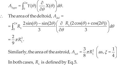
With this minimum amount of information, the two robots can calculate the path policies of each other, as well as the common intersecting path ( $P_{i} \cap P_{j}$ ) and common nodes, with respect to the current position. The robot with a lower priority will retreat to one of the nearby nodes, which does not lie in the path of the robot with a higher task priority.

Once the robot with a lower priority has moved out of the intersecting path, the other robot will resume its motion. If the priorities are equal, or if there is no priority assigned, other schemes can be employed to prioritize a robot. For example, the ratio of the length of the path already traversed by the robot and the length of the path still to be traversed can be calculated, while the robot with a higher ratio can be prioritized, or vice versa. The centres of a deltoid or an astroid can also be used as retreat points for the robots provided that their area ( $A_{h y p o}$ ) is safely lesser than the area of the robot.

The area of the hypocycloid is given by:

\begin{array}{l} A_{h y p o} = \int_{0}^{2 π} Y (θ) (\frac{\partial}{\partial θ} X (θ)) d θ . \\ ∴ & The area of the deltoid, A_{d e l} = \\ = \int_{0}^{2 π} R_{L} \frac{2 \sin (θ) - \sin (2 θ)}{3} (\frac{\partial}{\partial θ} \frac{R_{L} (2 \cos (θ) + \cos (2 θ))}{3}) d θ \\ = \frac{2}{9} π R_{L}^{2} . \\ Similarly, the area of the astroid, A_{a s t} = \frac{3}{8} π R_{L}^{2} (as, ξ = \frac{1}{4}) \\ In both cases, R_{L} is  defined by Eq.5 . \end{array}

It may happen that the lower priority robot has no nearby node to retreat to. This leads to a deadlock situation, in which both robots are stuck, with neither able to retreat. In this case, the robot with the higher priority retreats to the nearest non-colliding safe node to avoid the deadlock condition.

5.1. Node caching and policy exchange

Calculation of the nearest safe node is avoided by ‵caching‵ the nodes. Each robot caches the nearest unoccupied node location as it traverses the path. Hence, when the robot encounters a collision situation with another robot, the cached safe node location is immediately available, meaning that a lot of computation is saved. Moreover, instead of calculating the overlapping paths ( $P_{i} \cap P_{j}$ ) between the two robots, the entire motion policies of the two robots themselves may be exchanged instead, which should save computation, but at the cost of more data communication.

6. Dynamic Obstacles and Map Update

Path planning is generally undertaken by taking the static obstacles of the map into consideration. However, there can also be dynamic obstacles in the map, which must be avoided by the robot. Avoidance by a mobile robot and humans has been proposed in various works, such as [58, 59]. In this paper, however, dynamic obstacles refer to obstacles that are not the part of static obstacles, but are instead placed later or displaced in the environment, for example, a chair or a box. Unlike moving people and pet animals, whose positions keep on changing in the environment, there is a high probability of other robots encountering the same dynamic obstacle in the same position. A robot can detect a dynamic obstacle in the map and calculate its coordinates in the global map with the sensors mounted on it. We use the JSON format to save the dynamic obstacle‵s coordinates with a Unix timestamp as follows:

Listing 2. Dynamic Obstacle Map Update

1 {“dynamic—obstacle”: { // Obstacle meta—data 2 “robot—id”: “01”, // Id of robot 3 “time—stamp”: “1440233037” // Unix time—stamp 4 “obstacles”: [ // Coordinates 5 {“obj1”: “x”: “786”, “y”: “99”, “1”:“20”, “w”:“73”}, 6 {“obj2”: “x”: “529”, “y”: “23”, “1”:“32”, “w”:“52”}] 7 } }

This JSON file is transferred to another robot, which parses the file using a JSON parser, and updates the coordinates of the obstacles in its map. This scheme is advantageous for two main reasons:

As other robots are only informed about the new obstacles‵ coordinates, they can update their maps instead of having to build the map by themselves. Only the bare minimum of information is communicated, as opposed to the entire map. The other robot can plan its path by taking into account the position of the new obstacles. This is efficient, not only in terms of the time saved to reach the destination, but also in terms of computation and battery power.

The timestamp ensures that the latest information about the obstacles is used to update the map, as timestamps can be compared easily.

Notice that the presented JSON file for updating the dynamic obstacle map only has geometric coordinates for the two dynamic obstacles, as we only use a laser range sensor. In the case of other sensors, such as visual sensors, other attributes of the dynamic obstacle, e.g., colour, could also be easily saved and communicated to other robots. Using timestamps requires that the clocks of the different robots are synchronized beforehand.

Figure 9.

Robots used in the experiments: (a) Pioneer P3DX; (b) Kobuki TurtleBot; (c) motion model of two-wheel differential drive robots

Figure 10.

Test environment with dimensions, grid map, SHP nodes and PRM paths: (a) environment (front view); (b) environment (side view); (c) dimensions of the map; (d) corresponding grid map; (e) SHP path with nodes; (f) the PRM result on the grid map

7. System Specifications

Two types of robots were used in the experiments: (1) a Pioneer P3DX [60] equipped with a UHG08LX laser range sensor [61] and (2) a Kobuki TurtleBot [62], which is equipped with a Microsoft Kinect sensor. Both are differential drive robots. The scanning area of the UHG08LX sensor is 270 degrees with 0.36 degrees/pitch. The detectable range varies from 0.02 to 8 m. The Kinect sensor consists of an RGB camera, a 3D depth sensor, a multi-array microphone and a motorized tilt. In this work, only the depth sensors are used to provide the input data for the TurtleBot. Its range is specified to be between 0.7 and 5 m. The field of view is 57 degrees horizontal and 43 degrees vertical, with a tilt range of ±27 degrees. Both sensors are known for their good performance and are well suited to indoor environments.

Each robot was equipped with a system running on a 64-bit Ubuntu Linux 14.04 operating system. Both robots were run on a Robot Operating System (ROS)[63], which has the capability to perform inter-node communication between the robots. The grid map of the environment was also created from depth data using the ROS. To parse the JSON files, we used the open source JSMN parser [64] due to its small code footprint and not having any dependencies.

8. Motion Model

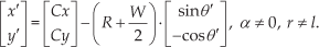
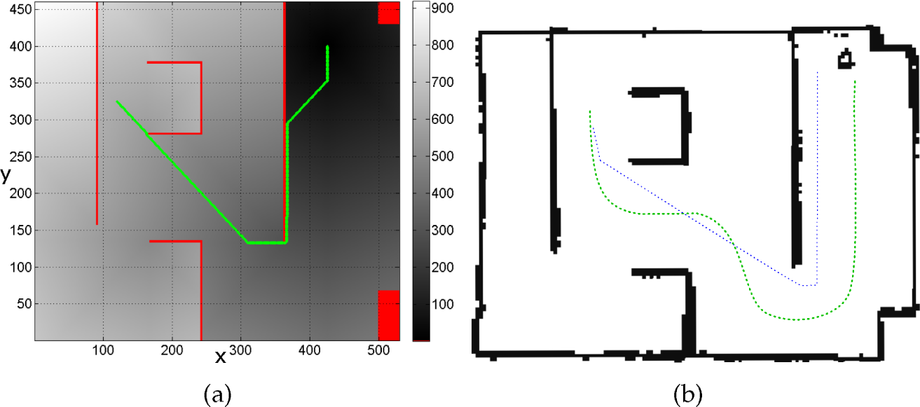
Both the P3DX and the TurtleBot used in the experiments are two-wheeled differential drive robots. Hence, we model the motion for a two-wheeled differential drive robot without slippage on surfaces with good traction. The distance between the left and the right wheel is W, while the robot state at position P is given as [ $x, y, θ$ ]. From Fig.9(c), turning angle α is calculated as:

\begin{array}{l} r = α \cdot (R + W), \\ l = α \cdot R \\ ∴ α = \frac{r - l}{W} \end{array}

(17)

and the radius of turn R as:

\begin{array}{l} R = \frac{l}{α}, α \neq 0. \end{array}

(18)

The coordinates of the centre of rotation (C, in Fig.9(c)), are calculated as:

[\begin{matrix} C x \\ C y \end{matrix}] = [\begin{matrix} x \\ y \end{matrix}] - (R + \frac{W}{2}) \cdot [\begin{matrix} sin θ \\ - cos θ \end{matrix}]

(19)

The new heading $θ^{'}$ is:

θ^{'} = (θ + α) mod 2 π,

(20)

from which the coordinates of the new position $P^{'}$ are calculated as:

[\begin{matrix} x^{'} \\ y^{'} \end{matrix}] = [\begin{matrix} C x \\ C y \end{matrix}] - (R + \frac{W}{2}) \cdot [\begin{matrix} sin θ^{'} \\ - cos θ^{'} \end{matrix}], α \neq 0, r \neq l .

(21)

If $r = l$ , i.e., if the robot motion is straight, the state parameters are given as:

θ^{'} = θ,

(22)

and:

\begin{array}{l} [\begin{matrix} x^{'} \\ y^{'} \end{matrix}] = [\begin{matrix} x \\ y \end{matrix}] + l \cdot [\begin{matrix} cos θ \\ sin θ \end{matrix}], (l = r) . \end{array}

(23)

9. Results

This section presents the results of smooth path generation, collision avoidance, deadlock avoidance, smooth path traversal in the case of a load carrying robot, dynamic obstacle avoidance with map update, and SHP with different δ.

For the sake of conciseness and readability, we represent the type of robot, its priority, and start and goal nodes as: C_tur^H::S⇝G, where S and G are the start and goal node locations, respectively. Subscript ‘tur’ denotes the TurtleBot, while ‘pio’ denotes the P3DX. H and L represent high and low priority, respectively.

Fig. 10(a) shows the environment used for the experiments. Fig. 10(b) shows the side view of the structured indoor environment with a regular non-slippery surface. The dimensions of the map are shown in Fig.10(c). The robot was moved in the environment, while the grid map shown in Fig.10(d) was constructed beforehand. A skeleton map is constructed from the grid map and the nodes are diffused as explained in Section 3 to generate hypocycloidal paths with the nodes (marked a,b,c,…) are shown in Fig.10(e). The probabilistic roadmap of the environment is shown in Fig.10(f). Both robots possessed the map and node information beforehand.

9.1. Experiment 1. SHP traversal and comparison with D* path traversal

The P3DX is initialized with configuration $C_{pio}^{H} : : c ⇝ s$ . The nodes ‵c‵ and ‵s‵ are shown in Fig.10(e). The D* algorithm calculates a path from start to goal, which is very close to the walls of the environment with sharp turns, as shown in Fig.11(a). Fig.11 shows the smooth hypocycloidal path traversed by the robot in green. For comparison, it also shows the D* path traversed by the robot. It can be seen that SHP path is not only smooth, but also maintains a safe distance from the obstacles.

9.2. Experiment 2: Collision avoidance on SHP nodes

9.2.1. Case A

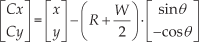
In Case A, the start and goal locations of each robot are different. The P3DX is initialized with configuration $C_{pio}^{H} : : s ⇝ w$ , whereas the TurtleBot is initialized with configuration $C_{tur}^{L} : : k ⇝ s$ (Fig.12(a)). The TurtleBot and the P3DX stop after sensing each other (Fig.12(b)) along the common path, and the low-priority TurtleBot retreats to the nearest cached node ‵l‵ (Fig.12(c)). Once the P3DX crosses over, it instructs the TurtleBot from node ‵m‵ to go ahead along the cleared path (Fig.12(e)). Finally, both robots stop at their respective goal locations (Fig.12(g)).

Figure 11.

Experiment 1. SHP vs. D* path traversal: (a) the D* path from start node ‵c‵ to goal node ‵s‵, with the intensity of the colour representing the proximity to the goal; (b) the dotted green line shows the traversed SHP path, while the dotted blue shows the traversed D* path. The D* path is very close to the obstacles, whereas the SHP path is not. Please refer to Video no. 1, 2 and 3 inTable 3.

Figure 12.

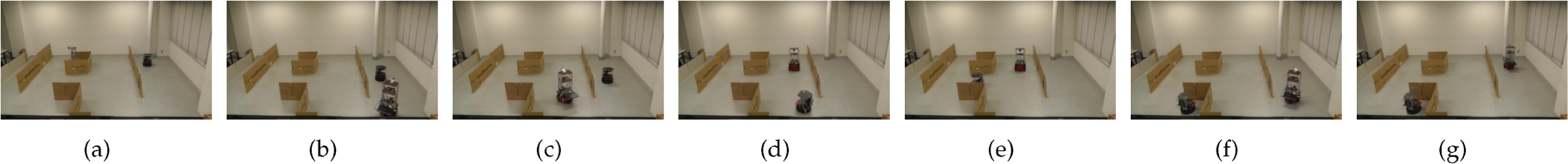
Experiment 2. (Case A) Collision avoidance on SHP nodes: (a) initial configuration of robots; (b) collision detection; (c) the low-priority TurtleBot retreats to cached safe node ‵l‵ (Fig.10(e)); (d,e) the P3DX continues towards its goal; (f,g) the TurtleBot moves towards its goal when the path is clear. Please refer to Video no. 4 inTable 3.

Figure 13.

Experiment 2. (Case B) Collision avoidance on SHP nodes: (a) initial configuration of robots; (b) collision detection; (c) the high-priority TurtleBot retreats to cached safe node ‵m‵ (Fig.10(e)), as P3DX has no non-overlapping safe node to retreat to; (d,e) P3DX continues towards its goal; (f,g) the TurtleBot moves towards its goal when the path is clear. Please refer to Video no. 5 inTable 3.

Figure 14.

Experiment 3. Avoiding Deadlock on SHP: (a) initial configuration of robots, with the P3DX starting early; (b) collision detection; (c) the high-priority P3DX retreats to cached safe node ‵l‵ (Fig.10(e)), as the low-priority TurtleBot has no non-overlapping safe node to retreat to; (d,e) the TurtleBot continues towards its goal; (f,g) the P3DX moves towards its goal when the path is clear. Please refer to Video no. 6 inTable 3.

9.2.2. Case B

In Case B, the start location of each robot is set as the goal location of the other robot, i.e., $C_{tur}^{H} : : k ⇝ s$ and $C_{pio}^{L} : : s ⇝ k$ (Fig.13(a)). Similar to Case A, both robots stop after sensing the presence of the other robot in the way (Fig.13(b)). Although the TurtleBot has higher priority, it still retreats to node ‵m‵ to avoid deadlock (Fig.13(c)), as there is no safe node for the P3DX to retreat to, which is not in the way of the TurtleBot. Once the P3DX crosses over, it instructs the TurtleBot from node ‵l‵ to go ahead along the cleared path (Fig.13(d)). Finally, both robots stop at their respective goal locations (Fig.13(g)).

9.3. Experiment 3. Avoiding deadlock on SHP

A deadlock situation can occur when a robot with low priority has no place to retreat to in order to clear the path for a robot with high priority. The initial configurations were set as follows: $C_{pio}^{H} : : a ⇝ s$ , and $C_{tur}^{L} : : s ⇝ w$ . In order to create a deadlock situation, the TurtleBot was programmed to start five seconds after the other robot had started. In the deadlock situation, as shown in Fig.14(b), there is no safe node for the TurtleBot to retreat to. Hence, the P3DX retreats to TurtleBot‵s non-colliding node ‘l’, then proceeds to its goal once the path has been cleared. The robots at the goals are shown in Fig.14(g). Notice that a similar deadlock situation was reached in Case B of Experiment 2, in which the robot with high priority retreated to avoid a deadlock.

9.4. Experiment 4. Dynamic obstacle avoidance on SHP

Robot paths can easily be planned with static obstacles in the map. However, obstacles can also be dynamic, while path planning may have to be done in real time. To test dynamic obstacle avoidance, the P3DX was initialized with $C_{pio}^{H} : : w ⇝ s$ and the return to the original position, i.e., $C_{pio}^{H} : : s ⇝ w$ (Fig.16(a)), while there were no dynamic obstacles in the environment. The motion policy generated by the robot at this point is shown in the PRM map of Fig.15(b) in green, such that the SHP path‵s goal nodes are: v,u,t,g,l,m,n,o,p,q,r and s, as shown in Fig.10(e). As soon as the robot starts its motion, two obstacles, X1 and X2, are manually placed in the environment shown in Fig.15(a). The robot stops after sensing the obstacle (Fig.16(c)) and a new motion policy is computed from the PRM map, which is shown in Fig.15(c), and the corresponding SHP, presented in Fig.10(e). The robot takes a detour via the new path (Fig.16(d) - 16(h)).

The position of the obstacles in the map is shown in Fig.15(a). The dimensions of the two obstacles ( $w i d t h \times b r e a d t h \times h e i g h t$ ) were:

$ObstacleX 1 : 32 \times 21 \times 73$ cm and

$ObstacleX 2 : 69 \times 27 \times 34$ cm.

Figure 15.

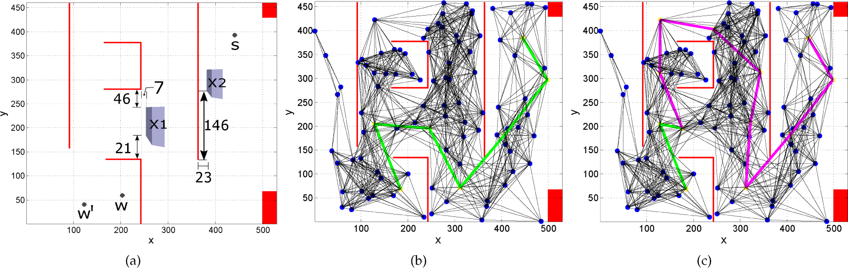
Experiment 4: Dynamic obstacle avoidance on SHP: (a) position of the two obstacles placed dynamically in the map; (b) initial path calculated by the PRM before dynamic obstacles were placed; (c) a new path calculated after sensing the dynamic obstacles

Figure 16.

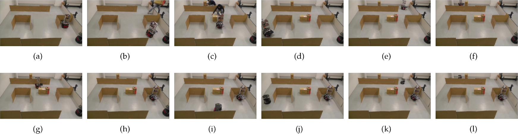
Experiment 4. Dynamic obstacle avoidance on SHP: (a) initial configuration; (b) the P3DX moves on the initially calculated short path; (c) the P3DX stops sensing the dynamic obstacles; (d) the P3DX calculates a new path and moves; (e,f,g) positions of the new obstacles are updated in the map; (h) the P3DX transfers the coordinates of the new obstacles to the TurtleBot; (i,j,k) the TurtleBot calculates the path with the updated map and moves. Please refer to Video no. 7 inTable 3.

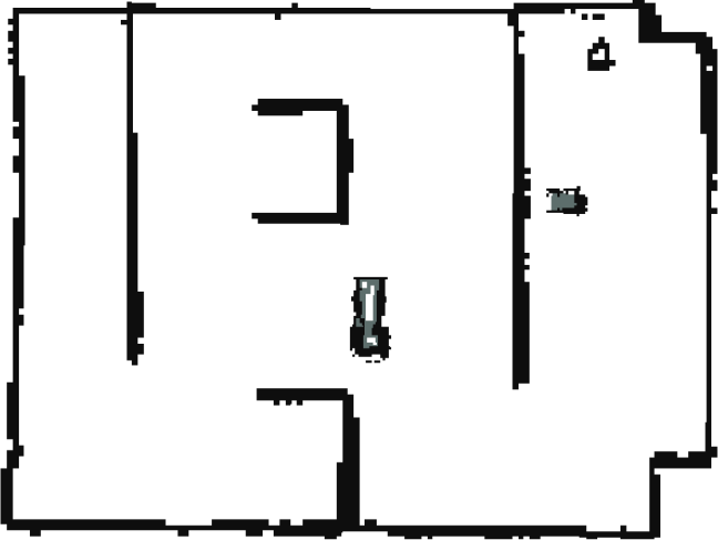
The P3DX updates the map with the new obstacle locations; once it returns to its start node w, it updates the TurtleBot stationed at node $w'$ (Fig.15(a)) about the positions of the obstacles in the map. Later, when the TurtleBot is initialized with $C_{tur}^{H} : : w' ⇝ s$ , it calculates the obstacle-free path towards the goal s, as shown in Fig.16(i)–16(l), using the updated map with new obstacles.

Figure 17.

Experiment 4. New grid map with dynamic obstacles.

9.5. Experiment 5. SHP with different clearance thresholds (δ)

SHP generation with different thresholds ( $δ_{i} \neq δ_{j}, i \neq j$ ) was shown earlier in Fig.5(a) and explained in Section 3. A different and modified environment, shown in Fig.18(a), was used to test SHP with different clearance thresholds. The dimensions of the new environment are shown in Fig.18(b), while the corresponding grid map is shown in Fig.18(c), which was also prepared beforehand. The same robot was first initialized with configuration $C_{pio}^{H} : : a ⇝ b$ and then with $C_{pio}^{H} : : a ⇝ c$ . In both cases, as the corner points P and Q are not collinear, while δ are different, the robot makes turns at different points of the SHP and maintains a clearance distance.

Figure 18.

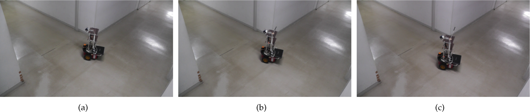
Experiment 5. SHP with different clearance thresholds (δ): (a) test environment; (b) dimensions of the environment (obstacle points P and Q are not collinear; for configuration $C_{pio}^{H} : : a ⇝ b$ , the P3DX takes a turn at node n₁, maintaining $δ = 60$ cm; for configuration $C_{pio}^{H} : : a ⇝ c$ , the P3DX takes a turn at node n₂, maintaining $δ = 70$ cm); (c) the grid map of the environment. Please refer to Video no. 8 inTable 3.

Figure 19.

Experiment 6. Obstacle avoidance on SHP with load carrying robots: (a) no load; (b) load length (centred) = 75 cm; (c) load length (centred) = 115 cm. Please refer to Video no. 9 inTable 3.

Figure 20.

Experiment 6. Obstacle avoidance on SHP with load carrying robots: (a) the grid map of the test environment, shown in Fig.19; (b) map dimensions with different SHP curves for different values of δ.

Figure 21.

SHP result comparison with QPMI [32], PRM and D*: (a) simulated environment; (b) skeleton map; (c) paths generated by QPMI, D*, PRM and SHP

9.6. Experiment 6. Obstacle avoidance on SHP with load carrying robots

The practical case of a robot carrying a load was also considered. A stick was fixed on the robot to simulate a load. Three experiments were performed with varying stick lengths, as follows: (a) 0 cm (i.e., no stick), (b) 75 cm (medium load) and (c) 115 cm (longest load). The clearance distance δ was set to 60 cm. Fig.19 shows the passage environment used for the experiment. Fig.20(a) shows the grid map of the environment. In the first experiment with no load (stick), the robot followed an SHP across the curve $\overset{⌢}{B B}$ '. When the load is medium-sized, the robot follows an SHP curve $\overset{⌢}{C C}$ ', while it follows the curve $\overset{⌢}{D D}$ ' for the longest load. The positions of the nodes are shown in Fig.20(b). The top view of the robot in the three scenarios is shown in Fig.19(a),Fig.19(b) and Fig.19(c). In all the three cases, the clearance of the robot was greater than clearance distance $δ = 60 cms$ , as summarized in Table 1. In all the experiments, we manually set the size of the load (stick) mounted on the robot.

10. Videos of the Results

The videos relating to all the experimental results presented in this paper can be downloaded from the Internet. The details of the videos are summarized in Table 3.

Table 1.

Load carrying robot on SHP with load width and actual clearance. For turn nodes, refer to Fig.20(b).

S. no.	Load width	Turn node	Clearance
1	No load	’A’	’67 cm’
2	75 cm	’C’	’61 cm’
3	115 cm	’D’	’65 cm’

11. SHP Comparison with Other Path Planning and Smoothing Techniques

We compared SHP with collision-free QPMI [32], along with D* [7] path planning and the PRM [9]. A smooth and collision-free path is proposed by S. R. Chang and U. Y. Huh in [32], which uses interpolation [27]. They first use a PRM algorithm to obtain linear waypoints on which the QPMI[31] algorithm is applied. However, the smooth path obtained from the QPMI algorithm may have points that collide with the obstacles; hence, they require a further collision check. If collisions are detected, they create a collision-free smooth path by realising a perpendicular line between the colliding point and the linear piecewise path joining the two PRM waypoints. The details of the algorithm can be found in [32, 31].

In order to compare the proposed SHP with collision-free QPMI, we replicated the simulation environment (shown in Fig.21(a)) presented by S. R. Chang and U. Y. Huh[32], using the same toolkit [65] used in their work. The intermediate skeleton map to create SHP is shown in Fig.21(b) for comparison and explanation purposes. Similar to the work in [32], the start location was fixed at the coordinates (5,5) and the goal location (95,95). Fig.21(c) respectively shows the results of paths generated by the D*, the PRM and QPMI[32] in dotted green, red and black, while the SHP are shown in blue.

The path generated by the D* algorithm is too close to the obstacles. Even if we shift the path by a distance equal to the width of the robot and some buffer, the path will still be angular. In the case of the PRM path, there are points ( $P_{1}, P_{2}$ and P₃) that are close to the obstacles. Moreover, the direct PRM path is not smooth. QPMI generates a smooth path. The circles on the QPMI path are the waypoints generated by the PRM algorithm, which are used to generate a smooth path using interpolation. There are points ( $Q_{1}, Q_{2}$ , and Q₃) in the QPMI path where free space is available, but the robot still comes close to the obstacles. On the other hand, the SHP path is not only smooth and continuous, it also maintains a better clearance from the obstacles. Originally, the point Q₃ is shifted right in the QPMI algorithm after collision detection (for details, refer to [32], page 9). However, considering the dimensions of the robot itself, it is still close. If we consider the straight passage between points A and B of the map, the robot should maintain an equal distance between the two walls in order to avoid coming close to either side of the walls. A wavy motion in the straight passage will obviously bring the robot close to one side of the wall at some points, which is not desired. The QPMI algorithm ends up generating undesired wavy paths in straight passages as it uses all the waypoints generated by the PRM algorithm, which are further smoothed using interpolation. On the other hand, SHP use skeleton maps (as shown in Fig.21(b)), which already generate straight pathways (passage AB is shown in Fig.21(b)) in corridors, and optimizes the paths at corners for the purpose of smoothing with the use of node diffusion.

Table 2.

Execution time for SHP generation (for a 100 × 100 pixels map of Fig.21); implementation in C++ on a 1.80GHz Intel Core-i7-4500CPU

Function	Time
Gridmap Binarize	3.0 msec
Gridmap Erode	3.2 msec
Gridmap Dilate	3.2 msec
Skeletonization (Algorithm of [47])	15.4 msec
Node clustering	13.6 msec
SHP curve generation on nodes	9.5 msec
Total	47.9 msec

The QPMI algorithm requires an explicit and computationally expensive collision detection, as well as trajectory changing steps, which are not required in SHP. Moreover, SHP are very fast: the SHP generation for the map shown in Fig.21 was completed in 48 msec without using any parallel programming. The time required for various sub-modules is summarized in Table 3. A parallel implementation would further reduce the computation time.

The diffused nodes in SHP can also act as points where a robot must retreat to in order to avoid collision with other robots in the case of multi-robot collision-free path planning, which is not considered in QPMI, the D* or the PRM. Moreover, neither the D*, the PRM nor QPMI algorithms consider the practical case of obstacle avoidance with load carrying robots, which is addressed in SHP. The major advantage of the proposed scheme is that it eliminates the need for a centralized controller for multiple robots. However, it is expensive in terms of waiting time as the robot has to wait on the safe nodes upon retreat. The overall time required to complete the tasks using multiple robots may also be larger than the centralized methods. However, since the decision to retreat and detour is taken in real time by local communication, it eliminates the need to recalculate the path of all the robots in case of dynamically changing the goal location (or tasks) of multiple robots.

A limitation of the proposed SHP in their purest form is that, for robots with high velocities, further smoothing in the transition from the straight line segment to the SHP curve for $G 2$ continuity may be required to be computed; to this end, we have proposed the use of transition curves.

Table 3.

Video list of all the experiments in this paper

Video no.	Experiment	Explanation	Download URL
1, 2, and 3	Exp. 1	SHP traversal (front view)SHP traversal (side-view)D* traversal	https://youtu.be/bvVEwbr4FWU
4 and 5	Exp. 2	Collision avoid (Case A)Collision avoid (Case B)	https://youtu.be/hVb6JUDLq7I
6	Exp. 3	Deadlock avoidance	https://youtu.be/IdJys3LbL4c
7	Exp 4.	Dynamic obstacle avoidance	https://youtu.be/RYnLK3TA19Y
8	Exp 5.	SHP with different δ	https://youtu.be/QDjWeO5SuEo
9	Exp. 6	SHP with load carrying	https://youtu.be/Hn2jJ50Zu4w

This study considered favourable surfaces with good wheel traction for the indoor wheeled robots used in the experiments. Moreover, ROS was used to control the wheeled robots. However, other types of surfaces need to be considered, particularly for outdoor robots. On slippery surfaces, wheel encoders will give false data, which can adversely affect a robot‵s localization in the map and ultimately the path planning. An estimation of the slip can help prevent errors in localization, as discussed in [66]. Path planning that considers wheel slip is discussed in [67]. For rough surfaces, the control system of the robot needs to be robust enough to cover the taxonomy of soil, rubble, grass and water. Path planning for rough surfaces is discussed in [68, 69]. A particularly interesting case, with regard to the presented work, is to consider wheel slip when a robot carries a load on slippery surfaces, as discussed in [70]. SHP evaluation on different types of surfaces is considered as a potential future project.

12. Conclusion

This paper has presented SHP for robot motion. SHP paths were generated at a safe distance from the environmental obstacles and avoided sharp turns, unlike the paths generated by the D* or PRM algorithm. A mathematical description of node diffusion with SHP generation was provided under different kinds of obstacles: in both cases, when the robot was carrying a load and when it was not. The paper introduced a novel motion policy in a parsable JSON format for robots, which could be exchanged with other robots for collision avoidance in a multi-robot scenario. In the proposed decoupled scheme to avoid multi-robot collision, robots communicate locally and decide to cross over or retreat to cached safe nodes to avoid collision. We showed how the nodes of the curved paths can be used as points for the robot to retreat to in order to avoid collision. We discussed cases of robot retreat with different priorities. In the case of dynamic obstacles, a decoupled approach was used to update other robots with the coordinates of the new and dynamic obstacles in the map. We tested the proposed techniques in real environments with multiple robots, as well as compared them with other path planning techniques. Experimental results show that the proposed SHP technique can generate smooth paths, which are desired for robot motion with collision avoidance involving multiple robots with different start and goal configurations. Robot motion on SHP in the case of moving entities, such as humans, is proposed as a potential future project. An extension of SHP for creating smooth 3D trajectories and an SHP evaluation on different types of surfaces are also under consideration.

Footnotes

13. Acknowledgements

This work is supported by the Ministry of Education, Culture, Sports, Science and Technology, Japan. We are thankful to the anonymous reviewers for giving us important suggestions to improve the manuscript.

References

Pollack

Maurice

Wiebenson

Walter

. Solutions of the shortest-route problem-a review. Operations Research, 8(2):224–230, 1960.

Hart

P.E.

Nilsson

N.J.

Raphael

, A formal basis for the heuristic determination of minimum cost paths. Systems Science and Cybernetics, IEEE Transactions on, 4(2):100–107, July 1968.

Tomás Lozano-Pérez Michael

A. Wesley

. An algorithm for planning collision-free paths among polyhedral obstacles. Commun. ACM, 22(10):560–570, October 1979.

Delling

Daniel

Sanders

Peter

Schultes

Dominik

Wagner

Dorothea

. Engineering route planning algorithms. In Lerner

Jürgen

Wagner

Dorothea

Zweig

KatharinaA.

, editors, Algorithmics of Large and Complex Networks, volume 5515 of Lecture Notes in Computer Science, pages 117–139. Springer Berlin Heidelberg, 2009.

LaValle

S. M.

, Planning Algorithms. Cambridge University Press, Cambridge, U.K., 2006. Available at http://planning.cs.uiuc.edu/, Accessed on 11 Feb 2016.

Latombe

Jean-Claude

. Robot Motion Planning. Kluwer Academic Publishers, Norwell, MA, USA, 1991.

Stentz

Anthony

Mellon

Is Carnegle

. Optimal and efficient path planning for unknown and dynamic environments. International Journal of Robotics and Automation, 10:89–100, 1993.

Stentz

Anthony

. The focussed d* algorithm for realtime replanning. In In Proceedings of the International Joint Conference on Artificial Intelligence, pages 1652–1659, 1995.

Kavraki

L.E.

Svestka

Latombe

J.-C.

Overmars

M.H.

, Probabilistic roadmaps for path planning in high-dimensional configuration spaces. Robotics and Automation, IEEE Transactions on, 12(4): 566–580, Aug 1996.

10.

Steven

M. Lavalle

. Rapidly-exploring random trees: A new tool for path planning. Technical report, 1998.

11.

LaValle

Steven M.

James

J. Kuffner

. Randomized kinodynamic planning. The International Journal of Robotics Research, 20(5):378–400, 2001.

12.

Hwang

Y.K.

Ahuja

, A potential field approach to path planning. Robotics and Automation, IEEE Transactions on, 8(1):23–32, Feb 1992.

13.

Dijkstra

E. W.

, A note on two problems in connexion with graphs. Numerische Mathematik, 1(1):269–271, 1959.

14.

Wang Shu-Xi . The improved dijkstra's shortest path algorithm and its application. Procedia Engineering, 29:1186–1190, 2012. 2012 International Workshop on Information and Electronics Engineering.

15.

Fujita

Nakamura

Shiller

, Dual dijkstra search for paths with different topologies. In Robotics and Automation, 2003. Proceedings. ICRA ′03. IEEE International Conference on, volume 3, pages 3359–3364 vol.3, Sept 2003.

16.

Steven

M. Lavalle

James

J. Kuffner

, and Jr. Rapidly-exploring random trees: Progress and prospects. In Algorithmic and Computational Robotics: New Directions, pages 293–308, 2000.

17.

Dubins

L. E.

, On curves of minimal length with a constraint on average curvature, and with prescribed initial and terminal positions and tangents. American Journal of Mathematics, 79(3):pp. 497–516, 1957.

18.

Dubins

Lester E.

, On plane curves with curvature. Pacific J. Math., 11(2):471–481, 1961.

19.

Fraichard

Scheuer

Alexis

. From reeds and shepp's to continuous-curvature paths. Robotics, IEEE Transactions on, 20(6):1025–1035, Dec 2004.

20.

Liscano

Green

, Design and implementation of a trajectory generator for an indoor mobile robot. In Intelligent Robots and Systems ′89. The Autonomous Mobile Robots and Its Applications. IROS ′89. Proceedings., IEEE/RSJ International Workshop on, pages 380–385, Sep 1989.

21.

Piazzi

Guarino Lo Bianco

Bertozzi

Fascioli

Broggi

, Quintic g2-splines for the iterative steering of vision-based autonomous vehicles. Intelligent Transportation Systems, IEEE Transactions on, 3(1):27–36, Mar 2002.

22.

Delingette

Hebert

Ikeuchi

, Trajectory generation with curvature constraint based on energy minimization. In Intelligent Robots and Systems ′91. ‘Intelligence for Mechanical Systems, Proceedings IROS ′91. IEEE/RSJ International Workshop on, pages 206–211 vol.1, Nov 1991.

23.

Komoriya

Tanie

, Trajectory design and control of a wheel-type mobile robot using b-spline curve. In Intelligent Robots and Systems ′89. The Autonomous Mobile Robots and Its Applications. IROS ′89. Proceedings., IEEE/RSJ International Workshop on, pages 398–405, Sep 1989.

24.

Takahashi

Hongo

Takero

Ninomiya

Sugimoto

Gunji

. Local path planning and motion control for agv in positioning. In Intelligent Robots and Systems ′89. The Autonomous Mobile Robots and Its Applications. IROS ′89. Proceedings., IEEE/RSJ International Workshop on, pages 392–397, Sep 1989.

25.

Choi

Ji wung

Curry

Elkaim

, Path planning based on bezier curve for autonomous ground vehicles. In World Congress on Engineering and Computer Science 2008, WCECS ′08. Advances in Electrical and Electronics Engineering - IAENG Special Edition of the, pages 158–166, Oct 2008.

26.

Yang

Kwangjin

Sukkarieh

, An analytical continuous-curvature path-smoothing algorithm. Robotics, IEEE Transactions on, 26(3):561–568, June 2010.

27.

Mathematical Interpolation. Wikipedia. 2015. Available at https://en.wikipedia.org/wiki/Interpolation, Accessed on 11 Feb 2016].

28.

Waring

Edward

. Problems concerning interpolations. Philoshopical Transactions Royal Society, 69(1): 59–67, 1779.

29.

Waring

Edward

. Problems concerning Interpolations. The Royal Society Publishing, London, U.K., 2015. Available at http://rstl.royalsocietypublishing.org/content/69/59.full.pdf+html, Accessed on 15 Jan 2016.

30.

James

F. Epperson

. On the runge example. Am. Math. Monthly, 94(4):329–341, April 1987.

31.

Huh

Uk-Youl

Chang

Seong-Ryong

. A g2 continuous path-smoothing algorithm using modified quadratic polynomial interpolation. International Journal of Advance Robot Systems, 11:25, doi:10.5772/57340, Oct 2013.

32.

Chang

Seong-Ryong

Huh

Uk-Youl

. A collision-free g2 continuous path-smoothing algorithm using quadratic polynomial interpolation. International Journal of Advance Robot Systems, 11:194, doi: 10.5772/59463, Sept 2014.

33.

Farin

Gerald

. Curves and Surfaces for CAGD: A Practical Guide. Morgan Kaufmann Publishers Inc., San Francisco, CA, USA, 5th edition, 2002.

34.

Svestka

Overmars

M. H.

, Coordinated path planning for multiple robots. Technical Report UU-CS-1996–43, Department of Information and Computing Sciences, Utrecht University, 1996.

35.

Ravankar

A. A.

Kobayashi

Jixin

Emaru

Hoshino

, An intelligent docking station manager for multiple mobile service robots. In Control, Automation and Systems (ICCAS), 2015 15th International Conference on, pages 72–78, Oct 2015.

36.

Guo

Parker

L.E.

, A distributed and optimal motion planning approach for multiple mobile robots. In Robotics and Automation, 2002. Proceedings. ICRA ′02. IEEE International Conference on, volume 3, pages 2612–2619, 2002.

37.

Yang

Dong-Hoon

Hong

Suk-Kyo

. A roadmap construction algorithm for mobile robot path planning using skeleton maps. Advanced Robotics, 21(1):51–63, 2007.

38.

Lockwood

E. H.

, Book of Curves. Cambridge University Press, 1961. Cambridge Books Online.

39.

Weisstein

Eric W.

, Hypocycloid from mathworld–a wolfram web resource. 2016. Available at http://mathworld.wolfram.com/Hypocycloid.html, Accessed on 3 Mar 2016.

40.

Sakellariou

Georgios

Shanahan

Murray

Kuipers

Benjamin

. Skeletonisation as mobile robot navigation. In In Proceedings of Towards Autonomous Robotic Systems (TAROS-04, pages 149–155, 2004.

41.

Arcelli

Carlo

Di Baja

Gabriella Sanniti

. A width-independent fast thinning algorithm. Pattern Analysis and Machine Intelligence, IEEE Transactions on, PAMI-7(4):463–474, July 1985.

42.

Bhattacharya

Gavrilova

M.L.

, Roadmap-based path planning - using the voronoi diagram for a clearance-based shortest path. Robotics Automation Magazine, IEEE, 15(2):58–66, June 2008.

43.

Ankit

A Ravankar

Hoshino

Yohei

Ravankar

Abhijeet

Jixin

Emaru

Takanori

Kobayashi

Yukinori

. Algorithms and a framework for indoor robot mapping in a noisy environment using clustering in spatial and hough domains. International Journal of Advanced Robotic Systems, 12, 2015.

44.

Ravankar

A. A.

Hoshino

Emaru

Kobayashi

, Map building from laser range sensor information using mixed data clustering and singular value decomposition in noisy environment. In System Integration (SII), 2011 IEEE/SICE International Symposium on, pages 1232–1238, Dec 2011.

45.

Anil

K. Jain

. Fundamentals of digital image processing. Prentice-Hall, Inc., Upper Saddle River, NJ, USA, 1989.

46.

Ravankar

Kobayashi

Ravankar

Emaru

, A connected component labeling algorithm for sparse lidar data segmentation. In Automation, Robotics and Applications (ICARA), 2015 6th International Conference on, pages 437–442, Feb 2015.

47.

Zhang

T. Y.

Suen

C. Y.

, A fast parallel algorithm for thinning digital patterns. Commun. ACM, 27(3): 236–239, March 1984.

48.

Bai

Xiang

Latecki

L.J.

Liu

Wen yu

. Skeleton pruning by contour partitioning with discrete curve evolution. Pattern Analysis and Machine Intelligence, IEEE Transactions on, 29(3):449–462, March 2007.

49.

Eric

W. Weisstein

. Cornu spiral from mathworld–a wolfram web resource. 2016. Available at http://mathworld.wolfram.com/CornuSpiral.html, Accessed on 15 Feb 2016.

50.

Eric

W. Weisstein

. Fresnel integrals from mathworld–a wolfram web resource. 2016. Available at http://mathworld.wolfram.com/FresnelInteg-rals.html, Accessed on 25 Feb 2016.

51.

Elbanhawi

Mohamed

Simic

Milan

Reza

N. Jazar

. Continuous path smoothing for car-like robots using b-spline curves. Journal of Intelligent & Robotic Systems, 80(1):23–56, 2015.

52.

Chang

Seong-Ryong

Huh

Uk-Youl

. Curvature-continuous 3d path-planning using qpmi method. International Journal of Advance Robot Systems, 11:194, doi:10.5772/60718, June 2015.

53.

Conway

R Howard

. The Transition-Curve Field-Book. Nabu Press, isbn:1245461192 edition, September 2011.

54.

Habib

Sakai

, Family of g2 cubic transition curves. In Geometric Modeling and Graphics, 2003. Proceedings. 2003 International Conference on, pages 117–122, July 2003.

55.

Ahmad

Gobithasan

Ali

J. M.

, G2 transition curve using quartic bezier curve. In Computer Graphics, Imaging and Visualisation, 2007. CGIV ′07, pages 223–228, Aug 2007.

56.

Ahmad

Ali

J. M.

, G3 transition curve between two straight lines. In Computer Graphics, Imaging and Visualisation, 2008. CGIV ′08. Fifth International Conference on, pages 154–159, Aug 2008.

57.

Srivastava

Roychowdhury

, Independent and interdependent latch setup/hold time characterization via newton raphson solution and euler curve tracking of state-transition equations. IEEE Transactions on Computer-Aided Design of Integrated Circuits and Systems, 27(5):817–830, May 2008.

58.

Hamasaki

Tamura

Yamashita

Asama

, Prediction of human's movement for collision avoidance of mobile robot. In Robotics and Biomimetics (ROBIO), 2011 IEEE International Conference on, pages 1633–1638, Dec 2011.

59.

Jiang

Rongxin

Tian

Xiang

Xie

Chen

Yaowu

. A robot collision avoidance scheme based on the moving obstacle motion prediction. In Computing, Communication, Control, and Management, 2008. CCCM ′08. ISECS International Colloquium on, volume 2, pages 341–345, Aug 2008.

60.

Pioneer P3-DX. Pioneer p3-dx robot. 2016. Available at http://www.mobilerobots.com/Libraries/Downloads/Pioneer3DX-P3DX-RevA.sflb.ashx, Accessed on 1 Mar 2016.

61.

UHG-08LX Technical Specifications. Uhg-08lx technical specifications. 2015. Available at http://www.autonomoustuff.com/hokuyouhg-08lx.html, Accessed on 2 Dec 2015.

62.

TurtleBot 2. Turtlebot 2 robot. 2015. Available at http://turtlebot.com, Accessed on 10 Oct 2015.

63.

Quigley

Morgan

Conley

Ken

Brian

P. Gerkey

Faust

Josh

Foote

Tully

Leibs

Jeremy

Wheeler

Rob

Andrew

Y. Ng. Ros

: An open-source robot operating system. In ICRA Workshop on Open Source Software, 2009.

64.

Zaitsev

Serge

. Jsmn Open Source JSON C Parser. Website, 2015. Available at https://bitbucket.org/zserge/jsmn/wiki/Home, Accessed on 9 Oct 2015.

65.

Corke

Peter

. Robotics, Vision and Control: Fundamental Algorithms in Matlab, volume 73. Springer, 2011.

66.

Jingang Yi Zhang

Junjie

Song

Dezhen

Jayasuriya

Suhada

. Imu-based localization and slip estimation for skid-steered mobile robots. In Intelligent Robots and Systems, 2007. IROS 2007. IEEE/RSJ International Conference on, pages 2845–2850, Oct 2007.

67.

Ishigami

Nagatani

Yoshida

, Path planning for planetary exploration rovers and its evaluation based on wheel slip dynamics. In Robotics and Automation, 2007 IEEE International Conference on, pages 2361–2366, April 2007.

68.

Spero

D. J.

Jarvis

R. A.

, Path planning for a mobile robot in a rough terrain environment. In Robot Motion and Control, 2002. RoMoCo ′02. Proceedings of the Third International Workshop on, pages 417–422, Nov 2002.

69.

ZakeriNejad

Bakhtiary

A. H.

Jahed Motlagh

M. R.

, Use of particle swarm optimization in path planning for rough terrain. In Robotics in Alpe-Adria-Danube Region (RAAD), 2010 IEEE 19th International Workshop on, pages 205–209, June 2010.

70.

Yokoyama

Matsuhasi

Sano

M. T.

, Slip control of a wheeled mobile robot with a movable auxiliary mass. In Advanced Intelligent Mechatronics (AIM), 2015 IEEE International Conference on, pages 1008–1013, July 2015.

SHP: Smooth Hypocycloidal Paths with Collision-Free and Decoupled Multi-Robot Path Planning

Abstract

Keywords

1. Introduction

2. Skeleton Map and Node Generation

3. Generating SHP

3.1. SHP for different angles

3.2. SHP curvature and continuity

4. Determining Clearance Distance (δ)

5. Multi-robot Path Planning on SHP

5.1. Node caching and policy exchange

6. Dynamic Obstacles and Map Update

7. System Specifications

8. Motion Model

9. Results

9.1. Experiment 1. SHP traversal and comparison with D* path traversal

9.2. Experiment 2: Collision avoidance on SHP nodes

9.2.1. Case A

9.2.2. Case B

9.3. Experiment 3. Avoiding deadlock on SHP

9.4. Experiment 4. Dynamic obstacle avoidance on SHP

9.5. Experiment 5. SHP with different clearance thresholds (δ)

9.6. Experiment 6. Obstacle avoidance on SHP with load carrying robots

10. Videos of the Results

11. SHP Comparison with Other Path Planning and Smoothing Techniques

12. Conclusion

Footnotes

13. Acknowledgements

References