Sage Journals: Discover world-class research

Abstract

This article introduces time-efficient path planning algorithms handling both path length and safety within a reasonable computational time. The path is planned considering the robot’s size so that as the robot traverses the constructed path, it doesn’t collide with an obstacle boundary. This article introduces two virtual robots deploying virtual nodes which discretize the obstacle-free space into a topological map. Using the topological map, the planner generates a safe and near-optimal path within a reasonable computational time. It is proved that our planner finds a safe path to the goal in finite time. Using MATLAB simulations, we verify the effectiveness of our path planning algorithms by comparing it with the rapidly-exploring random tree (RRT)-star algorithm in three-dimensional environments.

Keywords

Fast path plan virtual robot topological map safe path plan

Introduction

Safe path planning is important for autonomous vehicle navigation. For real-time applications, it is required that a path planner finds a safe solution path within a reasonable amount of time. This article introduces novel path planning algorithms handling both path length and safety within a reasonable computational time.

There are many papers on path planning of an autonomous vehicle.^1

–7 A-star or Dijkstra algorithms^1
–3 divide the workspace into multiple grid cells. As the workspace size increases, the number of grid cells required to represent the workspace also increases. It is well-known that the computational load of the A-star or Dijkstra algorithms increases considerably as we increase grid sizes or environment complexity. Thus, computing a path using A-star or Dijkstra algorithms in a large complex environment may not be feasible.

A-star or Dijkstra algorithms use grids with blocked and unblocked cells to represent terrain. However, paths formed by grid edges can be suboptimal and unrealistic looking, since the possible headings are artificially constrained. Thus,^8,9 presented any-angle path planning on grids such that paths are not constrained to grid edges.

The original A-star algorithm was later further extended to bidirectional A-star search,^10,11 where two separate unidirectional A-star searches are carried out simultaneously from both the start and the goal. A forward A-star search is carried out from the start toward the goal, while a backward A-star search is carried out from the goal toward the start.

There are many path planning methods which are used in environments without grid cells.^{4,5,12

–21} For instance, a Voronoi diagram can be used to build a safe path for a robot in two dimensions.^{12

–19,22} However, a Voronoi diagram path may be unnecessarily long, especially in a situation where a passage between two obstacles is too wide.

Many path planning algorithms, such as RRT-star,^4,5 used random sampling to generate a path in environments without grid cells. RRT-star approaches can easily handle three-dimensional (3-D) space and nonholonomic constraints, such as robot arm manipulators and steering.²⁰ The solution constructed by RRT-star converges to the optimum solution asymptotically by spending infinite time.⁵ However, waiting for infinite time is not possible in practice. This inspired us to develop path planning algorithms which can generate a near-optimal path within a reasonable amount of time.

Recall that paths formed by grid edges can be suboptimal and unrealistic looking, since the possible headings are artificially constrained.^8,9 This problem doesn’t occur in the proposed approach, since we consider path planning which doesn’t require grid cells. This article introduces novel path planning algorithms handling both path length and safety within a reasonable computational time.

In the literature on robotics, there are many papers on multi-robot systems.^{23

–36} Coordinating multiple robots can be utilized in many tasks, such as sensor network building, surveillance, exploration, intruder capture, rendezvous, or formation control.

The proposed path planning method was developed inspired by multi-robot networking algorithms in the study by Kim.^18,19,23,37 The purpose of the work by Kim^18,19,23,37 was to use multiple robots deploying nodes so that the complete network is built as fast as possible. The major distinction from the work by Kim^18,19,23,37 is that this article handles building a safe path to the goal as fast as possible. Another distinction from the work by Kim^18,19,23,37 is that this article considers virtual robots which can move with infinite speed. Note that a real robot cannot move with infinite speed. However, a virtual robot can move with infinite speed, since a virtual robot exists in simulations and is used to build a path using simulations.

Among many papers on path planning of robots, our approach is novel in using unique concepts, such as virtual robots and virtual nodes. Initially, two virtual robots are deployed at the goal and the start, respectively. A forward search by one virtual robot is carried out from the start toward the goal, while a backward search by another virtual robot is carried out from the goal toward the start. This bidirectional search is developed inspired by bidirectional A-star search in the literature.^10,11

Once two virtual robots are deployed, then they keep deploying virtual nodes which discretize the obstacle-free space into a topological map. In other words, the virtual robots deploy virtual nodes so that the network structure, called the traversible graph, can be built in the environments. Here, traversible graph satisfies that an edge in the graph can be traversed by a robot safely without collision, since the edge is not blocked by an obstacle.

Once the traversible graph is built, then we search for a shortest path between the start and the goal using the graph. This way, our planner generates a safe and near-optimal path within a reasonable computational time. We plan a path considering the robot’s size so that as the robot traverses the constructed path, it doesn’t collide with an obstacle.

In the literature,^4,5,20 tree may expand randomly to any direction, not toward the goal directly. However, this random expansion may slow down the process of finding a path to the goal. A-star algorithms use heuristics to guide its search toward the goal. The proposed path plan strategy is similar to A-star algorithms,¹ since under our approach, a virtual robot tries to move toward its destination directly if it is possible. This direct movement is used to find a path between the start and the goal in a time-efficient manner.

It is proved that our planner based on two virtual robots generates a safe path to the goal in finite time. Using MATLAB simulations, we verify the effectiveness of our path planning algorithms by comparing it with the RRT-star algorithm in 3-D environments.

The organization of this article is as follows. The second section introduces assumptions and definitions. The third section presents our path planning algorithms using virtual robots. The fourth section shows simulation results to verify the effectiveness of our algorithms. The fifth section provides conclusions.

Assumptions and definitions

We consider a workspace with obstacles. Let goal denote a point in an obstacle-free space. Let us assume that the location of the goal is known to a robot. The problem to be solved in this article is as follows: build a safe path from the start to the goal so that a robot can arrive at the goal as fast as possible while avoiding collision.

Consider the case in which we build a safe path for a robot whose size can be approximated as a sphere with radius r. We use two virtual robots, R ₁ and R ₂, in order to plan the path of the real robot. Here, R_i , where $i \in \{1, 2\}$ , is a spherical virtual robot with radius r. Let R_i denote the position of R _i .

R ₁ starts from the start point, and R ₂ starts from the goal point. R ₁ searches for a path to the goal point, and R ₂ searchers for a path to the start point. The goal point is set as the destination of R ₁. Also, the start point is set as the destination of R ₂.

We say that R_i collides with an obstacle in the case where the sphere, centered at R _i , with radius r intersects an obstacle boundary.

Let $L i n e (n_{1}, n_{2})$ denote a straight line segment whose two end points are two locations given by n ₁ and n ₂, respectively. Let $d i s t (n_{1}, n_{2})$ denote the length of $L i n e (n_{1}, n_{2})$ .

We say that $L i n e (n_{1}, n_{2})$ is a collision-free path once the following condition is met: while R_i traverses $L i n e (n_{1}, n_{2})$ , R_i doesn’t collide with an obstacle.

R_i iteratively deploys virtual nodes on its way so that the connected network is built. Virtual nodes discretize the obstacle-free space into a topological map. Each virtual node has spherical sensing coverage with radius $r_{\max}$ .

It is assumed that in the case where a node detects another node, the two nodes can communicate with each other. This implies that the communication range is longer than the sensing range. This assumption was also used in the study by Kim.^18,19,37 Also, the communication and sensing abilities of a node begin working once the node is deployed. This approach of using robots deploying nodes is inspired by multi-robot networking algorithms in the study by Kim.^18,19,37

Recall that R_i iteratively deploys virtual nodes on its way so that the connected network is built. Let the traversible graph I_i be defined by a set $I_{i} = (V (I_{i}), E (I_{i}))$ . Here, $V (I_{i})$ is the vertex set and $E (I_{i})$ is the edge set.

Every vertex in $V (I_{i})$ represents a virtual node deployed by R_i . Every edge, say $\{n_{1}, n_{2}\} \in E (I_{i})$ , indicates that $L i n e (n_{1}, n_{2})$ is a collision-free path and that $d i s t (n_{1}, n_{2}) \leq N_{c} r_{\max}$ . Here, n _j indicates the position of a node n_j , and $N_{c} > 1$ is a constant. Since $L i n e (n_{1}, n_{2})$ is a collision-free path, an edge in the traversible graph can be traversed by a robot safely without collision, since the edge is not blocked by an obstacle.

$N_{c} > 1$ implies that the upper bound for the edge length is bigger than the maximum sensing range $r_{\max}$ . Recall that each virtual node has spherical sensing coverage with radius $r_{\max}$ .

N_c is a tuning parameter for our path planning. As N_c increases, the graph I_i becomes denser by having more edges. As the graph becomes denser, we can find a shorter path using the graph I_i .

See Figure 1 for an illustration. This figure depicts I_i as N_c varies. In the case where $N_{c} = 1.1$ , I_i is composed of three edges (bold edges in Figure 1). However, in the case where $N_{c} = 3$ , I_i is composed of six edges. As we use $N_{c} = 3$ , the shortest path, from A to B, in I_i is the straight line segment.

Figure 1.

This figure depicts I_i as N_c varies. In the case where $N_{c} = 1.1$ , I_i is composed of three edges (see bold edges in the figure). However, in the case where $N_{c} = 3$ , I_i is composed of six edges. As we use $N_{c} = 3$ , the shortest path, from A to B, in I_i is the straight line segment.

Since an edge in $E (I_{i})$ is a collision-free path for R_i , R_i can traverse any edge in $E (I_{i})$ infinitely fast. Thus, we say that R_i jumps from one node in I_i to another node in I_i instantly. Based on the definition of $E (I_{i})$ , R_i doesn’t collide with an obstacle while traversing an edge in $E (I_{i})$ .

Suppose that $v_{1} \in V (I_{1})$ and $v_{2} \in V (I_{2})$ satisfy the following condition: $L i n e (v_{1}, v_{2})$ is a collision-free path, and $d i s t (v_{1}, v_{2}) \leq N_{c} r_{\max}$ . In this case, we generate the combined graph $I = (V (I), E (I))$ as follows: $V (I) = V (I_{1}) \cup V (I_{2})$ . An edge $\{n_{1}, n_{2}\}$ in $E (I)$ implies that the following condition is met: $L i n e (n_{1}, n_{2})$ is a collision-free path, and $d i s t (n_{1}, n_{2}) \leq N_{c} r_{\max}$ .

Once the combined graph is built, then we say that I ₁ and I ₂ are connected to each other. We also say that $I = I_{1} + I_{2}$ . We further say that two nodes n ₁ and n ₂ are adjacent in the case where $\{n_{1}, n_{2}\} \in E (I)$ .

Recall that each virtual node has spherical sensing coverage with radius $r_{\max}$ . This implies that a virtual node n emits infinite number of sensor rays (with maximum length $r_{\max}$ ) surrounding n to detect a nearby obstacle. Let footPrint of a node n denote the 3-D space where the sensor ray of n can reach while not being blocked by an obstacle. Let coverBoundary of a node n denotes the boundary of the footprint of n.

Some points on the coverBoundary of n exist on obstacle boundaries, since a sensor ray of n can be blocked by an obstacle. In the case where the sensors of the node n detect no obstacles, the footprint becomes the sphere whose center corresponds to n and the radius of which is $r_{\max}$ .

An openSpace of n denotes the set of points on the coverBoundary of n, which are not on obstacle boundaries. An openFront of n is the subset of an openSpace such that all points on the openFront are not inside a footPrint of any other node. In the case where every node has no openFront, the footPrints of all nodes cover the entire workspace.

We need to simulate a node n emitting many sensor rays surrounding n. Suppose that the virtual node n emits q ² sensor rays surrounding n to detect a nearby obstacle. Here, q is a positive integer. Then, we generate q ² points on the coverBoundary of n. As q increases, we obtain densely spaced points on the coverBoundary.

Suppose that a node n emits q ² sensor rays surrounding n to detect a nearby obstacle. Then, q ² points are generated on the coverBoundary of n. We use this generation method in our MATLAB simulations (see the “Simulation results” section).

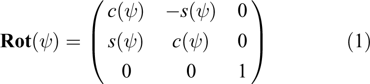
Consider a unit vector $[1, 0, 0]$ . We first rotate this unit vector by one angle among $[2 × π / q,4 × π / q,6 × π / q ..., 2 π]$ about the z-axis. The counterclockwise rotation of ψ about the z-axis is represented by the following rotation matrix $R o t (ψ)$

R o t (ψ) = (\begin{matrix} c (ψ) & - s (ψ) & 0 \\ s (ψ) & c (ψ) & 0 \\ 0 & 0 & 1 \end{matrix})

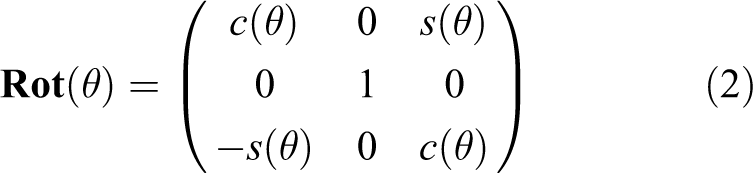
Then, we rotate the resulting vector by one angle among $[2 π / q,4 × π / q,6 × π / q ..., 2 π]$ about the y-axis. The counterclockwise rotation of θ about the y-axis is represented by the following rotation matrix $R o t (θ)$

R o t (θ) = (\begin{matrix} c (θ) & 0 & s (θ) \\ 0 & 1 & 0 \\ - s (θ) & 0 & c (θ) \end{matrix})

The resulting vector after two rotations is

f p (ψ, θ) = R o t (ψ) R o t (θ) {[1, 0, 0]}^{T}

$f p (ψ, θ)$ presents the unit vector representing one sensor ray after rotations ψ and θ. The ray starts from n, and it may meet an obstacle boundary or not. Considering the maximum sensing range $r_{\max}$ , the sensor ray is represented as the following line segment

L_{n} (ψ, θ) = L i n e (n, n + f p (ψ, θ) × r_{\max})

Let $p_{ψ, θ}$ denote a point on the coverBoundary, which is associated to two rotations ψ and θ. We derive $p_{ψ, θ}$ as

p_{ψ, θ} = n + f p (ψ, θ) × r a y D i s t (ψ, θ)

Here, $r a y D i s t (ψ, θ)$ is set as follows. If $L_{n} (ψ, θ)$ in equation (4) doesn’t meet an obstacle boundary, then we set

r a y D i s t (ψ, θ) = r_{\max}

Otherwise, we set

r a y D i s t (ψ, θ) = ‖ n - d (ψ, θ) ‖

Here, $d (ψ, θ)$ is the intersection where $L_{n} (ψ, θ)$ meets an obstacle boundary.

Recall that both ψ and θ are selected from q values, respectively. Thus, in total, q ² points are generated using equation (5).

See Figure 2 for an illustration of $p_{ψ, θ}$ . In this figure, the ray is depicted with an arrow emitted from n. The ray doesn’t meet an obstacle. Thus, $r a y D i s t (ψ, θ) = r_{\max}$ using equation (6). According to the definition of the openSpace, $p_{ψ, θ}$ in Figure 2 is on the openSpace.

Figure 2.

An illustration of $p_{ψ, θ}$ . In this figure, the ray is depicted with an arrow emitted from n. The ray doesn’t meet an obstacle. Thus, $r a y D i s t (ψ, θ) = r_{max}$ using equation (6).

Let $p_{g o a l}$ denote the goal position. Also, let $p_{s t a r t}$ denote the start position.

Recall that $p_{g o a l}$ is the destination of the virtual robot R ₁. Thus, for R ₁, we define the closestPoint(1) as the point whose coordinate is

p_{c 1} = n + \frac{r_{\max} (p_{g o a l} - n)}{‖ p_{g o a l} - n ‖}

Recall that $p_{s t a r t}$ is the destination of the virtual robot R ₂. Thus, for R ₂, we define the closestPoint(2) as the point whose coordinate is

p_{c 2} = n + \frac{r_{\max} (p_{s t a r t} - n)}{‖ p_{s t a r t} - n ‖}

For the virtual robot $R_{i} (i \in \{1, 2\})$ , the closestPoint(i) and q ² points ( $p_{ψ, θ}$ in equation (5)) are called the candidate FrontierPoints of n. See Algorithm 2. Among these $q^{2} + 1$ candidate FrontierPoints, we select a set of FrontierPoints, $f (n)$ , on an openFront satisfying the following condition: there exists a collision-free path connecting n and a point in $f (n)$ . This condition is called the condition for a FrontierPoint.

Algorithm 2.

R_i . $F r o n t i e r G e n e r a t e (n)$ .

The above condition implies that R_i doesn’t collide with an obstacle boundary while R_i moves from n to any point in $f (n)$ . This condition is required, since R_i uses a FrontierPoint as a “way-point” to reach its destination.

Path planning

A time-efficient path planning algorithm is presented in Algorithm 1. This section presents the algorithm in detail.

Algorithm 1 iterates until a node in I ₁ is connected to a node in I ₂. Once I ₁ is connected to I ₂, then we generate a new combined graph $I = I_{1} + I_{2}$ . We then build a path from the start to the goal using I. This path becomes the path for the real robot to reach the goal.

Figure 3 illustrates R_i deploying a new node. In this figure, R_i is a sphere-shaped robot. The robot moves inside a tunnel in this figure. The tunnel boundaries are depicted with red curves, and the trajectory of the robot is depicted with a yellow curve. The large dots on the trajectory of the robot indicate the nodes deployed by the robot. 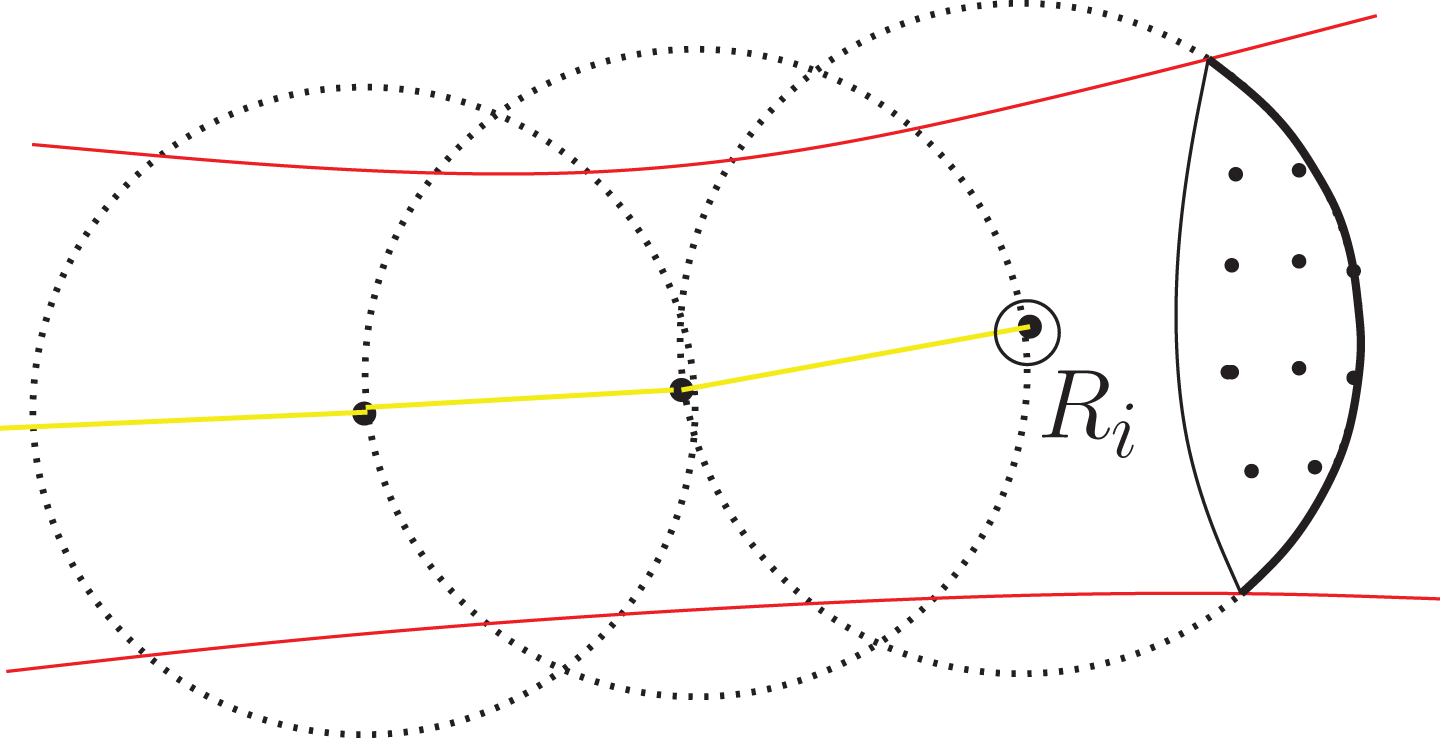The maximum sensing range of each node is depicted as a dotted sphere with radius $r_{\max}$ . FrontierPoints are marked as large dots on the coverBoundary of one node.

Figure 3.

R_i deploying a new node. The maximum sensing range of each node is depicted as a dotted sphere with radius $r_{max}$ . FrontierPoints are marked as large dots on the coverBoundary of one node.

Using I_i , R_i searches for a node, say $n \in V (I_{i})$ , with a FrontierPoint. Note that the distance between R_i and n doesn’t matter, since R_i is a virtual robot and jumps to n instantly. Once n is found, then R_i jumps to n.

Let $f_{R_{i}}$ denote a FrontierPoint of n, which R_i will visit after jumping to n. In the case where n has the closestPoint(i) as a FrontierPoint, then the closestPoint(i) is set as $f_{R_{i}}$ . Otherwise, we randomly select one FrontierPoint of n as $f_{R_{i}}$ . Suppose that n has M FrontierPoints, say $\{f^{1}, f^{2},..., f^{M}\} \in f (n)$ , in total. We randomly select one number from the list $\{1, 2, ..., M\}$ . Suppose we selected $m \in \{1, 2, ..., M\}$ . This case, $f^{m} \in f (n)$ is selected as $f_{R_{i}}$ .

Since we select a random FrontierPoint, the path plan result changes as we run Algorithm 1 multiple times. This random selection is presented in Algorithm 3, which is a sub-algorithm of Algorithm 1. Once $f_{R_{i}}$ is selected, then R_i jumps to $f_{R_{i}}$ .

Algorithm 3.

R_i . $F r o n t i e r S e a r c h$ .

R_i visits the closestPoint(i) of n before visiting other FrontierPoints of n. In other words, R_i moves toward its destination directly if it is possible. This direct movement is used to search for a feasible path in a time-efficient manner.

This movement toward the destination distinguishes our article from tree expansion strategies in the literature.^4,5,20 In the literature,^4,5,20 tree may expand randomly to any direction, not toward the goal directly. Since R_i moves toward its destination directly if it is possible, the computational efficiency of our path plan strategy increases considerably. The proposed path plan strategy is similar to A-star algorithms,¹ since A-star algorithms use heuristics to guide its search toward the goal.

Once R_i reaches $f_{R_{i}}$ , then it deploys a new node at $f_{R_{i}}$ . Whenever a new node, say n, is deployed, every FrontierPoint within $r_{\max}$ distance from n is deleted. Also, n is connected to the traversible network I_i and I_i includes the node. R_i then searches for a node with a FrontierPoint using I_i .

Algorithm 4 presents the path planning from the start to the goal using the traversible graph I. We use the Dijkstra algorithm which finds the shortest path along the traversible graph I. (The Dijkstra algorithm is optimal in finding the shortest path. The A-star algorithm uses a heuristic function to guide its search toward the goal. As far as the authors know, the A-star is suboptimal in finding the shortest path, due to this heuristic function.)

Algorithm 4.

$B u i l d P a t h (S, G, I)$ .

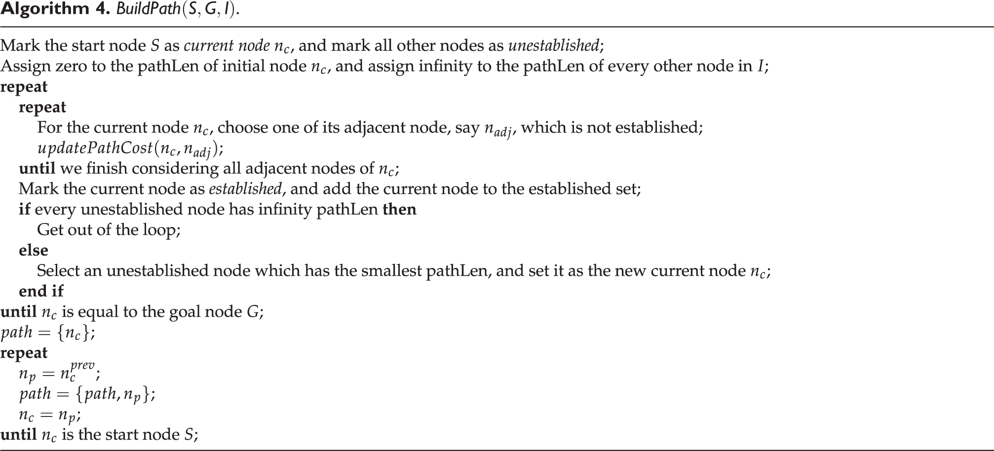
We explain Algorithm 4 briefly. Recall that two nodes n ₁ and n ₂ are adjacent in the case where $\{n_{1}, n_{2}\} \in E (I)$ . Also, recall that $d i s t (n_{1}, n_{2})$ is the length of $L i n e (n_{1}, n_{2})$ . In Algorithm 4, we say that a node n is established in the case where a shortest path from the start to n is established.

The pathLen of a shortest path, say $(n_{1}, n_{2},..., n_{k})$ , is defined as

p a t h L e n (n_{k}) = \sum_{i = 2}^{k} d i s t (n_{i - 1}, n_{i})

Equation (10) results in

p a t h L e n (n_{k}) = p a t h L e n (n_{k - 1}) + d i s t (n_{k - 1}, n_{k})

u p d a t e P a t h C o s t (n_{c}, n_{a d j})

in Algorithm 5 is used to update the cost of

n_{a d j}

based on equation (11). In Algorithm 5,

n_{a d j}^{p r e v}

denotes the previous node of

n_{a d j}

along the shortest path to

n_{a d j}

. In the case where n_c is the previous node of

n_{a d j}

along the shortest path to

n_{a d j}

, equation (11) leads to

Algorithm 5.

$u p d a t e P a t h C o s t (n_{c}, n_{a d j})$ .

p a t h L e n (n_{a d j}) = p a t h L e n (n_{c}) + d i s t (n_{c}, n_{a d j})

which is presented in Algorithm 5.

Analysis

In this subsection, we analyze the performance of our algorithms theoretically.

Recall the definition of FrontierPoints as follows. Among $q^{2} + 1$ candidate FrontierPoints, we select a set of FrontierPoints $f (n)$ on an openFront satisfying the following condition: there exists a collision-free path between n and a point in $f (n)$ .

For this analysis, we consider the case where a sensor coverage is infinitesimally small ( $r_{\max} \approx 0$ ) and q goes to infinity. This case, FrontierPoints of n, $f (n)$ , converges to an openFront of n.

The following theorem proves that in the case where R_i cannot find an openFront, the entire obstacle-free space is covered by footPrints.

Theorem 1

In the case where R_i cannot find an openFront, the entire obstacle-free space is covered by footPrints.

Proof

Using the transposition rule, we prove the following statement: in the case where an obstacle-free space, which is not covered by footPrints, exists, then R_i can find an openFront.□

Suppose that an obstacle-free space, which is not covered by footPrints, exists. Let O denote this uncovered obstacle-free space. According to the definition of an openFront, at least one node has an openFront along the boundary of O. Thus, R_i can find this openFront.

Theorem 1 implies that in the case where R_i cannot find an openFront, the entire obstacle-free space is covered by footPrints. Thus, I ₁ and I ₂ are connected to each other before R_i cannot find an openFront. This implies that Algorithm 1 proceeds until I ₁ and I ₂ are connected to each other.

Theorem 2 proves that the real robot doesn’t collide with an obstacle boundary as it traverses edges in $I = I_{1} + I_{2}$ .

Theorem 2

As the real robot traverses edges in I, it doesn’t collide with an obstacle boundary.

Proof

Using the definition of I, every edge, say $\{n_{1}, n_{2}\} \in E (I)$ , indicates that $L i n e (n_{1}, n_{2})$ is a collision-free path. As the real robot traverses edges of I, it doesn’t collide with an obstacle.□

The real robot doesn’t collide with an obstacle boundary as it traverses the path built using Algorithm 1. In Algorithm 1, Algorithm 4 generates a path to the goal using the traversible graph I. While the real robot traverses edges of I until meeting the goal, the robot doesn’t collide with an obstacle boundary using Theorem 2.

Simulation results

This section verifies the performance of Algorithm 1 using extensive simulations. The real robot’s initial position is $(30, 30, 30)$ . The goal position is $(170, 170, 170)$ . Also, we set $N_{c} = 5$ and $q = 36$ . The radius of a robot is $r = 5$ distance units. This implies that we plan the safe path for a spherical robot with radius $r = 5$ distance units.

We compare the proposed algorithm with the RRT-star algorithm in the study by Sertac and Emilio.⁵ The settings of the RRT-star algorithm are as follows. Two nodes are neighbors in the case where the distance between the two nodes is smaller than 10 distance units. The step size (expansion of the tree within one time step) in the RRT-star algorithm is set as 10 distance units.

The solution constructed by the RRT-star algorithm converges to the optimum solution asymptotically by spending infinite amount of time.⁵ Since we cannot wait for infinite time, we finish the RRT-star algorithm in the case where the relative distance between the constructed node and the goal position is smaller than 10 distance units.

Fifty Monte-Carlo simulations are implemented to verify the performance of our method rigorously. This article uses two metrics for comparison with the RRT-star algorithm. The first metric is the computational time. Let $C T^{t} (t \in \{1, 2, ..., 50\})$ denote the computational time (in seconds) using the tth Monte-Carlo simulation. We use $M e a n (C T) = \frac{\sum_{i = 1}^{50} C T^{t}}{50}$ . Also, we use $M i n (C T) = m i n_{t \in {1, 2, ..., 50}} C T^{t}$ . We further use $M a x (C T) = m a x_{t \in {1, 2, ..., 50}} C T^{t}$ . The second metric is the length of the generated path. Let $L^{t} (t \in \{1, 2, ..., 50\})$ denote the constructed path length using the tth Monte-Carlo simulation. We use $M e a n (L) = \frac{\sum_{i = 1}^{50} L^{t}}{50}$ . Also, we use $M i n (L) = m i n_{t \in {1, 2, ..., 50}} L^{t}$ . We further use $M a x (L) = m a x_{t \in {1, 2, ..., 50}} L^{t}$ .

In Algorithm 3, we randomly select one FrontierPoint of n as $f_{R_{i}}$ . Recall that $f_{R_{i}}$ denotes a FrontierPoint of n, which R_i will visit after jumping to n. Thus, as we use 50 random Monte-Carlo simulations, we generate 50 distinct paths. Moreover, we perform extensive simulations while changing $r_{\max}$ in the “The effect of changing $r_{\max}$ ” section. Using extensive simulations, we show that randomly generated paths avoid collision in a robust manner.

Figure 4. depicts the cluttered environment considered in the simulations. Each obstacle has a spherical shape.

Figure 4.

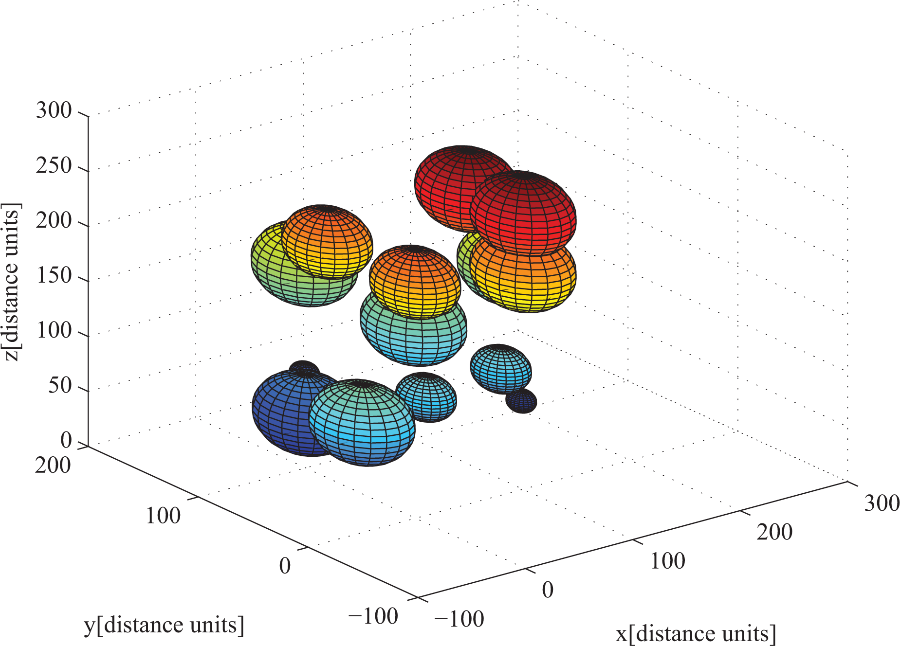
Each obstacle has a spherical shape.

Table 2 presents the analysis of both the proposed method (Algorithm 1) and the RRT-star. In the proposed planning method, we set $r_{\max}$ as 50 distance units. $[P R O]$ is used to represent the proposed method. Also, $[R R T]$ is used to represent the RRT-star algorithm. See that Algorithm 1 generates a shorter path than the RRT-star algorithm. Moreover, Algorithm 1 runs faster than the RRT-star algorithm. This shows that Algorithm 1 outperforms the RRT-star algorithm.

The effect of changing $r_{\max}$

This subsection presents the effect of changing $r_{\max}$ in Algorithm 1. Table 2 presents the analysis. See that the computational load (simulation time) increases as we decrease $r_{\max}$ . However, decreasing $r_{\max}$ doesn’t necessarily decrease the generated path length.

Table 1.

The analysis of both the proposed method and the RRT-star.

$A l g .$	$M e a n (C T)$	$M i n (C T)$	$M a x (C T)$	$M e a n (L)$	$M i n (L)$	$M a x (L)$
$[P R O]$	280	252	327	1.89	1.46	2.89
$[R R T]$	348	310	406	3.97	3.53	4.53

Algorithm 1.

Path plan strategy.

Table 2.

The effect of changing $r_{max}$ in Algorithm 1.

$r_{max}$	$M e a n (L)$	$M e a n (C T)$
100	295	0.61
90	296	0.78
80	282	0.95
70	282	1.11
60	274	1.44
50	282	1.95
40	284	2.33

Conclusions

This article introduces novel path planning algorithms handling both path length and safety within a reasonable computational time. The proposed planner is based on unique concepts such as virtual robots and virtual nodes.

Initially, two virtual robots are deployed at the goal and the start, respectively. A forward search by one virtual robot is carried out from the start toward the goal, while a backward search by another virtual robot is carried out from the goal toward the start.

Two virtual robots deploy virtual nodes which discretize the obstacle-free space into a topological map. Using the topological map, the planner generates a safe and near-optimal path within a reasonable computational time. It is proved that our planner finds a safe path to the goal in finite time.

Using MATLAB simulations, we verify the effectiveness of our path planning algorithms by comparing it with the RRT-star algorithm. As our future works, we will do experiments using autonomous aerial vehicles to verify the effectiveness of the proposed approach.

The proposed planning method can be applied in two-dimensional (2-D) environments, as well as in 3-D environments. In 2-D environments, a virtual robot has a circular shape instead of spherical shape. Also, sensor coverage is depicted as a circle in 2-D case. In 2-D environments, FrontierPoints are generated on circles, instead of spheres. Then, the path plan algorithms in this article can still be applied.

As our future works, we will extend the proposed planning method to the path planning of an industrial robot arm. There are many papers on the path planning of an industrial robot arm.^{38

–45} For a robot with d degrees-of-freedom (DOF), the configuration space (c-space) represents each DOF as a dimension in its coordinate system. Each d-dimensional point in the c-space represents the d joint angles of the robot. Due to this property, motion planning in the c-space is simpler than that in geometric spaces. A motion planning task involves connecting two points in the c-space, with obstacles mapping from the Cartesian space to the c-space using forward-kinematic collision checks.⁴⁶ Once the c-space is given, then the proposed planning method, which is extended to d dimensional space, can be applied to search for a safe path in the c-space. The extension of the proposed planning method to $d (d > 3)$ dimensional space will be done as our future works.

Footnotes

Declaration of conflicting interests

The author(s) declared no potential conflicts of interest with respect to the research, authorship, and/or publication of this article.

Funding

The author(s) disclosed receipt of the following financial support for the research, authorship, and/or publication of this article: This work was supported by the National Research Foundation (NRF) of Korea grant funded by the Korea government (MSIT) (no. 2019057282).

ORCID iD

Jonghoek Kim

References

Choset

Lynch

Hutchinson

, et al. Principles of robot motion. Cambridge, England: MIT Press, 2005.

Kim

Choo

. Stealth path planning for a high speed torpedo-shaped autonomous underwater vehicle to approach a target ship. Cyber Phys Syst 2018; 4: 1–16.

Pettie

. A new approach to all-pairs shortest paths on real-weighted graphs. Theor Comput Sci 2004; 312(1): 47–74.

Kuffner

LaValle

. Space-filling trees: a new perspective on incremental search for motion planning. In: Proceedings IEEE international conference on intelligent robots and systems, San Francisco, CA, 25–30 September 2011, pp. 2199–2206.

Karaman

and Frazzoli

. Sampling-based algorithms for optimal motion planning. Int J Robot Res 2011; 30(7): 846–894.

Kim

. Control laws to avoid collision with three dimensional obstacles using sensors. Ocean Eng 2019; 172: 342–349.

Plonski

Tokekar

Isler

. Energy-efficient path planning for solar-powered mobile robots. Heidelberg, Germany: Springer, 2013, pp. 717–731.

Munoz

Rodriguez Moreno

. Improving efficiency in any-angle path-planning algorithms. In: 2012 6th IEEE international conference intelligent systems, Sofia, Bulgaria, 6–8 September 2012, pp. 213–218.

Nash

Daniel

Koenig

, et al. Theta*: any-angle path planning on grids. In: AAAI’07 Proceedings of the 22nd national conference on artificial intelligence, vol. 2, Canada, September 2007, pp. 1177–1183.

10.

Ikeda

Hsu

Imai

, et al. A fast algorithm for finding better routes by AI search techniques. In: Proceedings of VNIS’94—1994 vehicle navigation and information systems conference, Japan, August 1994, pp. 291–296.

11.

Koll

Kaindl

. Bidirectional best-first search with bounded error: summary of results. In: Proceedings of the 13th international joint conference on artificial intelligence, IJCAI’93, vol. 1, France, 28 August–3 September 1993, pp. 217–223. San Francisco, CA: Morgan Kaufmann Publishers Inc.

12.

Kim

Zhang

Egerstedt

. A provably complete exploration strategy by constructing Voronoi diagrams. Auton Robot 2010; 29(3–4): 367–380.

13.

Choset

Walker

Eiamsa Ard

, et al. Sensor-based exploration: incremental construction of the hierarchical generalized Voronoi graph. Int J Robot Res 2000; 19(2): 126–148.

14.

Nagatani

Choset

. Toward robust sensor based exploration by constructing reduced generalized Voronoi graph. In: Proceedings of IEEE/RSJ international conference on intelligent robots and systems, Kyongju, Korea, 17-21 October 1999, pp. 1687–1692.

15.

Choset

Burdick

. Sensor-based exploration: the hierarchical generalized Voronoi diagram. Int J Robot Res 2000; 19: 96–125.

16.

Choset

Nagatani

. Topological simultaneous localization and mapping (SLAM): toward exact localization without explicit localization. IEEE Trans Robot Automat 2001; 17: 125–137.

17.

Kim

Zhang

Egerstedt

. Simultaneous cooperative exploration and networking based on Voronoi diagrams. In Proceedings of IFAC workshop on networked robotics, Colorado, USA, 6–8 October 2009, pp. 1–6.

18.

Kim

. Cooperative exploration and protection of a workspace assisted by information networks. Ann Math Artif Intell 2014; 70(3): 203–220.

19.

Kim

. Capturing intruders based on Voronoi diagrams assisted by information networks. Int J Adv Robot Syst 2017; 14(1): 1–8.

20.

Yershov

LaValle

. Improving motion planning algorithms by efficient nearest-neighbor searching. IEEE Trans Robot 2007; 23(1): 151–157.

21.

Sprunk

Lau

Pfaffz

, et al. Online generation of kinodynamic trajectories for non-circular omnidirectional robots. In 2011 IEEE international conference on robotics and automation, Shanghai, China, 9–13 May 2011, pp. 72–77.

22.

Kim

. Workspace exploration and protection with multiple robots assisted by sensor networks. Int J Adv Robot Syst 2018; 15(4): 1–14.

23.

Kim

. Multirobot exploration while building power-efficient sensor networks in three dimensions. IEEE Trans Cybern 2018; 49(7): 1–8.

24.

Ajorlou

Momeni

Aghdam

. A class of bounded distributed control strategies for connectivity preservation in multi-agent systems. IEEE Trans Autom Control 2010; 55(12): 2828–2833.

25.

Dimarogonas

Johansson

. Decentralized connectivity maintenance in mobile networks with bounded inputs. In Proceedings of IEEE international conference on robotics and automation, Pasadena, CA, 19–23 May 2008, pp. 1507–1512.

26.

Ando

Oasa

Suzuki

, et al. Distributed memoryless point convergence algorithm for mobile robots with limited visibility. IEEE Trans Robot Autom 1999; 15: 818–828.

27.

Flocchini

Prencipe

Santoro

, et al. Gathering of asynchronous robots with limited visibility. Theor Comput Sci 2005; 337: 147–168.

28.

Cortés

Martnez

Bullo

. Robust rendezvous for mobile autonomous agents via proximity graphs in arbitrary dimensions. IEEE Trans Autom Control 2006; 51(8): 1289–1298.

29.

Lin

Morse

Anderson

BDO

. The multi-agent rendezvous problem. In Proceedings of IEEE international conference on decision and control, Maui, HI, USA, 9–12 December 2003, pp. 1508–1513.

30.

Egerstedt

. Distributed coordination control of multi-agent systems while preserving connectedness. IEEE Trans Robot 2007; 23(4): 693–703.

31.

Roza

Maggiore

Scardovi

. A class of rendezvous controllers for underactuated thrust-propelled rigid bodies. In: Proceedings of IEEE international conference on decision and control, USA, 15–17 December 2014, pp. 1649–1654.

32.

Park

Hutchinson

. A distributed optimal strategy for rendezvous of multi-robots with random node failures. In: Proceedings of IEEE international conference on intelligent robots and systems, USA, 14–18 September 2014, pp. 1155–1160.

33.

Kim

. Three-dimensional multi-robot control to chase a target while not being observed. Int J Adv Robot 2019; 16(1): 1729881419829667.

34.

Kim

. Three-dimensional discrete-time controller to intercept a targeted UAV using a capture net towed by multiple aerial robots. IET Radar Sonar Navig 2019; 13: 682–688.

35.

Peng

Akella

. Coordinating multiple robots with kinodynamic constraints along specified paths. Intl J Robot Res 2005; 24(4): 295–310.

36.

Janchiv

Batsaikhan

Kim

, et al. Time-efficient and complete coverage path planning based on flow networks for multi-robots. Int J Control Autom Syst 2013; 11(2): 369–376.

37.

Kim

. Cooperative exploration and networking while preserving collision avoidance. IEEE Trans Cyber 2017; 47(12): 4038–4048.

38.

Shiller

. Time-energy optimal control of articulated systems with geometric path constraints. In: Proceedings of the 1994 IEEE international conference on robotics and automation, vol. 4, San Diego, CA, May 1994, pp. 2680–2685.

39.

Shiller

Dubowsky

. On the optimal control of robotic manipulators with actuator and end-effector constraints. In: Proceedings of 1985 IEEE international conference on robotics and automation, vol. 2, St. Louis, MO, 25–28 March 1985, pp. 614–620.

40.

Chen

. Haptic-aided robot path planning based on virtual tele-operation. Robot Comput Integr Manuf 2009; 25(4): 792–803.

41.

Cao

Dodds

Irwin

. Constrained time-efficient and smooth cubic spline trajectory generation for industrial robots. IEE Proc Control Theor Appl 1997; 144(5): 467–475.

42.

Chettibi

Lehtihet

Haddad

, et al. Minimum cost trajectory planning for industrial robots. Eur J Mech A/Solids 2004; 23(4): 703–715.

43.

Saravanan

Ramabalan

. Evolutionary minimum cost trajectory planning for industrial robots. J Intell Robot Syst 2008; 52(1): 45–77.

44.

Bobrow

Dubowsky

Gibson

. Time-optimal control of robotic manipulators along specified paths. Int J Robot Res 1985; 4(3): 3–17.

45.

Shin

McKay

. Minimum-time control of robotic manipulators with geometric path constraints. IEEE Trans Autom Control 1985; 30(6): 531–541.

46.

Das

Gupta

Yip

. Fastron: an online learning-based model and active learning strategy for proxy collision detection. In: Conference on robot learning, USA, 13–15 November 2017, pp. 496–564.

Time-efficient path planning using two virtual robots

Abstract

Keywords

Introduction

Assumptions and definitions

Path planning

Analysis

Theorem 1

Proof

Theorem 2

Proof

Simulation results

The effect of changing r max

Conclusions

Footnotes

Declaration of conflicting interests

Funding

ORCID iD

References

The effect of changing $r_{\max}$