Strategic Path Planning by Sequential Parametric Bayesian Decisions

Abstract

The objective of this research is to generate a path for a mobile agent that carries sensors used for classification, where the path is to optimize strategic objectives that account for misclassification and the consequences of misclassification, and where the weights assigned to these consequences are chosen by a strategist. We propose a model that accounts for the interaction between the agent kinematics (i.e., the ability to move), informatics (i.e., the ability to process data to information), classification (i.e., the ability to classify objects based on the information), and strategy (i.e., the mission objective). Within this model, we pose and solve a sequential decision problem that accounts for strategist preferences and the solution to the problem yields a sequence of kinematic decisions of a moving agent. The solution of the sequential decision problem yields the following flying tactics: “approach only objects whose suspected identity matters to the strategy”. These tactics are numerically illustrated in several scenarios.

1. Introduction

Classification is an act of allocating an entity into a category on the basis of its properties. In this paper, we achieve optimal classification by judiciously making kinematic decisions for a mobile agent that minimizes the expected risk of the classification outcome. The risk of each classification outcome is determined by a loss function, whose weight is dictated by the preference of a strategist (or a policy maker) who defines the mission objective. The approach is parametric since the loss function is considered as a design variable of the mission and we use Bayesian inference to process the collected information. The problem is solved sequentially such that the solution provides a sequence of kinematic decisions that constitute a path.

1.1. Motivation

Unmanned Aerial Vehicles (UAVs) have proved to be an invaluable force multiplier for the Joint Force Commander (JFC) [1]. It is predicted that the UAV market is to more than double over the next decade [2] where UAVs can provide both persistent and highly capable intelligence, surveillance and reconnaissance (ISR) [1]; ISR capability is therefore the number one combatant commander priority for UAVs in the U.S. Army [3].

Every military operation has a strategist who decides the desired strategic goals of the mission where the goals are to be achieved by applying military resources and means, such as UAVs. The actual strategy must be incorporated effectively so that all the resources are fully exploited in the service of the strategic goals. The motivation of this work is to optimize the couplings between several operational components beginning with the decisions of the strategist, continuing with the kinematic decisions of the mobile agent, followed by the information collection by the sensors carried by the agent, and ending with the classification decisions taken by the agent.

1.2. Mission Overview

In a given area, there are a number of objects of interest whose locations and categories (i.e., target or non-target) are known a priori but memberships are not. An agent equipped with sensors, e.g., Electro-Optical (EO) and infrared (IR), is used to collect information with respect to the objects and classify the objects based on the gathered information. The onboard sensors are imperfect in that the probability of detection decreases as the distance between the sensor and the object increases. The agent's time is constrained due to limited fuel and it has a priori information of the total number of targets in the area provided by intelligence. A strategist decides the loss function associated with each faulty classification decision made by the agent. In other words, the strategist determines the priority of the objectives as there can be many objectives within a mission, and such a priority directly influences the next-level tactical decisions (e.g., if the object is a target, what further actions do we take?). The objective is to generate a path for the agent that optimizes the strategic objectives that account for misclassification and the consequences of misclassification where the weights assigned to these consequences are chosen by the strategist.

1.3. Literature Review

Much work has been done previously under the broad topic of probabilistic decision making in UAV operations. In [4], the authors investigated the use of human operator feedback for target recognition in an ISR scenario where a team of Micro Aerial Vehicles (MAVs) is assigned to fly over a number of objects of interest and the operator must decide whether or not the object is a target. In [5], the authors presented decision making strategies under uncertainty and adversary action for the Cooperative Operations in UrbaN TERrain program (COUNTER), where stochastic dynamic programming was employed to optimize the resource allocation. In [6], the problem of path planning for a UAV in the presence of radar-guided surface-to-air missiles was investigated. The radar model was formulated probabilistically, and the optimal strategy obtained in this work confirmed the standard flying tactics such that an aircraft should “deny range, aspect and aim”.

With an information-theoretic measure, one can quantify information using the probabilities associated with the outcomes of the situation at hand. In [7], the author investigated the use of Shannon's information [8] in performance and requirement estimation in multisensor fusion applications. A set of heuristics was developed to relate the information content and recognition performance of a sensor system by using Johnson's criteria [9]. In [10], optimal sensor parameter selection in a static visual system was studied with the optimality criterion as the reduction of uncertainty in the state estimation process using Shannon's mutual information. In [11], sensor management in a dynamic environment was examined where the authors used an active sensing approach that combines particle filtering, predictive density estimation, and relative entropy maximization.

1.4. Original Contributions

The original contributions of this work are as follows.

1. We propose a model that accounts for the interaction between the agent kinematics, informatics, classification and strategy.

2. Within this model, we pose and solve a sequential decision problem that accounts for strategist preferences and the solution to the problem yields a sequence of kinematic decisions of a moving agent.

3. The solution of the sequential decision problem yields the following flying tactics: “approach only objects whose suspected identity matters to the strategy”. These tactics are numerically illustrated in several scenarios.

1.5. Relevance to Past Work

Previously, we posed a problem where the mission of the unmanned vehicle was to travel through a given area and collect a specified amount of information about each object of interest while minimizing the total mission time [12]. Shannon's channel capacity [8] was utilized as a model for information collection. An optimal control problem was posed and the necessary conditions for optimality of the path were analytically derived. Furthermore, numerical results were illustrated on several time-optimal cooperative exploration scenarios. This method was developed for vehicles equipped with range-based sensors and travelling in an uncertain area [13]. In [14], time-optimal paths are generated for a vehicle to collect specified amounts of information about objects of interest at known locations using noisy anisotropic sensors. Trajectories are sought to improve information collection by finding trade-offs amongst the couplings between kinematics, informatics and estimation; the approach was validated by a hardware demonstration using a three-wheeled ground robot.

In the presence of multiple non-isotropic objects whose information collection rates are not constant with respect to the relative positions between the agent and the object, finding a feasible path that satisfies the mission specification can be challenging. The bond energy algorithm [15] is an optimization heuristic that iteratively improves infeasible path conditions to feasible ones for multiple non-isotropic objects. In [16], we investigated the path planning strategies of a Dubins vehicle with several (range-based) sensor configurations. In [17, 18], we studied the optimal informative path planning with Bayesian classification that accounts for the couplings between kinematics, informatics and classification.

The presented work is an extension of our previous work and we investigate the path planning of a mobile agent that accounts for the couplings between the agent kinematics, informatics, classification and strategy.

1.6. Paper Outline

The remainder of the paper is as follows. In Section 2, the modelling for kinematics, informatics and classification are presented, and the risk function that is used as the cost function is formulated using the notion of confusion matrix. In Section 3, an optimization problem is formulated such that the risk function is to be minimized with respect to the kinematic and classification decisions. In Section 4, the risk function for different outcomes of the action variable is derived and loss function candidates for interesting mission scenarios are presented. In Section 5, numerical simulation results are given. The conclusion and future work are discussed in Section 6.

2. Modelling

The agent comprises three relevant subsystems: kinematics, informatics and classification. In this section, we present the model for each subsystem. The strategy is treated separately to the agent's subsystems (Sec. 2.5), as it defines the mission objective.

2.1. Kinematics

We assume that the physical world that the agent explores is a Manhattan gridded space. The area of interest is represented by a grid made from the intersection of horizontal and vertical lines with equal spacing. An agent is located on the intersection of the lines (vertex) and it moves along the lines of the grid (edges). There are four choices of movement direction which are up, down, left and right. The agent moves from one vertex to another adjacent vertex depending on the direction it chooses.

Let us define a decision variable φ, which describes the agent's action on the direction it chooses to go. There are five possible outcomes for φ, which are up, down, left, right and stay. Abstracting each action with its first character, i.e., u for up, φ is defined as

$\varphi \in \left\{u\mathrm{,}d\mathrm{,}l\mathrm{,}r\mathrm{,}s\right\}.$

2.2. Informatics

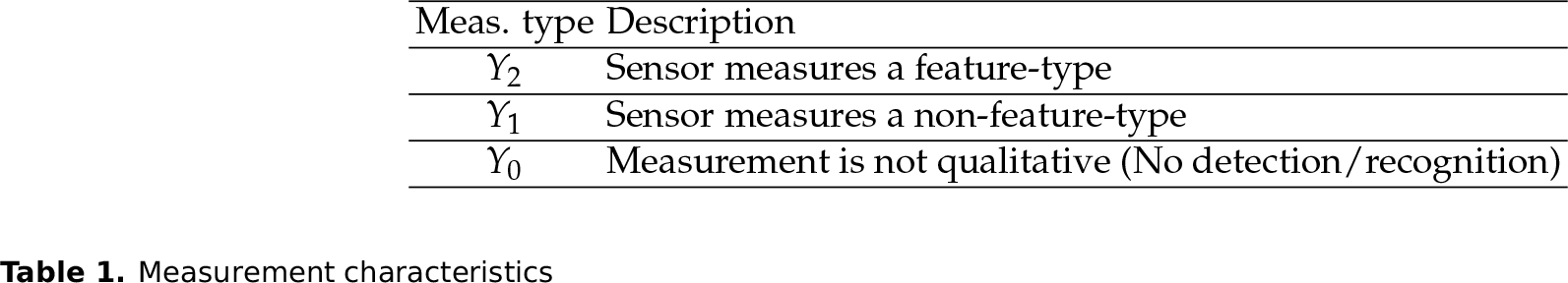
We define two events which are the property of the object (X) and the measurement type (Y), respectively. For the object property X ∊ {T, NT} where X = T denotes an event where an object of interest is a target, while X = NT denotes the object of interest being a non-target. For the measurement type, Y ∊ {Y₀, Y₁, Y₂} and Table 1 show the summary of the events. Feature-type (Y₂) is an attribute of a target while non-feature-type (Y₁) is an attribute of a non-target. An object possesses several attributes which are recognized visually by the agent. These attributes are categorized by either one of the three outcomes, as shown in the table, by using statistical pattern recognition techniques [18].

Table 1.

Measurement characteristics

Meas. type	Description
Y 2	Sensor measures a feature-type
Y 1	Sensor measures a non-feature-type
Y 0	Measurement is not qualitative (No detection/recognition)

2.2.1. Property of Object

The probability of the object being a target and the probability of the object being a non-target are defined as

$P\left(X=T\right)=p,P\left(X=NT\right)=1-p,$

(1)

where p ∊ [0, 1]. These are the a priori probabilities in the Bayesian sense. In practice, this information is given by intelligence obtained prior to the mission.

2.2.2. Likelihood Functions & Constraint

Given the two events, X and Y, the conditional probability of Y given X is formulated as follows.

$P\left(Y=Y_i|X\right)={\sigma }_{iX}$

(2)

where 0 ≤ σ ≤ 1 and i ∊ {0,1,2}.

Based on the fact that the sample space probability must equal to one, i.e., P(Ω) = 1, one can derive the following equation using the product rule.

$p\left({\sigma }_{0T}+{\sigma }_{1T}+{\sigma }_{2T}\right)+\left(1-p\right)\left({\sigma }_{0NT}+{\sigma }_{1NT}+{\sigma }_{2NT}\right)=1$

(3)

This is a constraint that the likelihood functions should satisfy in order to be proper functions.

2.2.3. Modified Performance Prediction Model

A performance prediction model for Electro-Optical (E-O) sensors is used as the measurement model for the agent. The modified performance prediction model (MPPM) for E-O systems is defined as the product of the target transfer probability function and the cross section probability.

$P_{MPPM}=P\left(r\right)·P_c\left(\theta \right)$

(4)

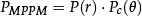
P(r) is the target transfer probability which describes the probability of successful discrimination (i.e., detection, recognition or identification [9]) as a function of the range between the sensor and the object to be classified.

$P\left(r\right)=\frac{{\left(N/N_{50}\right)}^E}{1+{\left(N/N_{50}\right)}^E}$

(5)

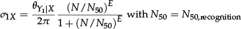
E = 2.7 + 0.7 (N/N₅₀) is obtained by fitting field test data, N₅₀ is the minimum resolution constant that gives 50% success rate of the chosen discrimination task (from Johnson's criteria [9]), N = ρd_c/r is the actual resolution of an object shown in the image plane. Here, ρ is the maximum resolvable spatial frequency, d_c is the characteristic target dimension, and r is the range from the sensor to the object. As the range between the sensor and the object shortens, the actual resolution of the object (N) increases, thus the probability of successful discrimination approaches 100%, i.e., r → 0, N → ∞, P(N) → 1, and vice versa. The performance is shown in Fig. 1. One important aspect is that depending on the chosen motion of the agent, the relative range to object(s) will vary, so the probability of successful discrimination will vary as well. Exploiting this aspect is the foundation of our approach to designing optimal control/decision strategies.

Figure 1.

Probability of discrimination tasks (i.e., detection, recognition and identification) with respect to range (in unit length)

The probability of successful discrimination is not only dependent on the range, but also on the orientation of the object. An object can be observed via various viewpoints, but only through the vantage point can the proper feature that classifies the property of the object be seen. This is analogous to observing dice sideways, where some of the sides have an ordinary pattern (non-feature) while the others have some particular ones (feature). Since the orientation of the object is unknown a priori, this aspect needs to be taken into account in the model. The cross section probability P_c is defined as

$P_c\left(Y=Y_1|X\right)=\frac{{\theta }_{Y_1|X}}{2\pi }$

(6a)

$P_c\left(Y=Y_2|X\right)=\frac{{\theta }_{Y_2|X}}{2\pi }$

(6b)

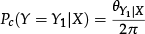
with 0 ≤ θ ≤ 2π where θ is the visible angle parameter (vantage point) at which the agent can observe the corresponding measurement type. This parameter may vary depending on the size of the target and the sampling rate of the measurement.

The completed modified performance prediction model describes the probability of successful discrimination as a function of the range (r) and the object property (X). We formulate the likelihood functions that were defined earlier, using the performance prediction model. The likelihood of measuring Y₀ is the probability of no detections, and it is identical regardless of the object property. On the other hand, the likelihood for measuring Y₁ and Y₂ correspond to the recognition level of a discrimination task and they are also functions of the object property. The following set of equations summarize the likelihood functions.

${\sigma }_0=1-P\left(r\right)=\frac{1}{1+{\left(N/N_{50}\right)}^E}\text{with} N_{50}=N_{\mathrm{50,}\text{detection}}$

(7a)

${\sigma }_{1X}=\frac{{\theta }_{Y_1|X}}{2\pi }\frac{{\left(N/N_{50}\right)}^E}{1+{\left(N/N_{50}\right)}^E} \text{with} N_{50}=N_{\mathrm{50,}\text{recognition}}$

(7b)

${\sigma }_{2X}=\frac{{\theta }_{Y_2|X}}{2\pi }\frac{{\left(N/N_{50}\right)}^E}{1+{\left(N/N_{50}\right)}^E} \text{with}\mathrm{,} N_{50}=N_{\mathrm{50,}\text{recognition}}$

(7c)

These likelihood functions are known functions obtained by calibration prior to the mission.

2.3. Classification

2.3.1. Snapshot

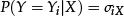
The Bayes theorem gives the posterior probability of an event (hypothesis) given evidence that supports the hypothesis. The posterior probability of an object being a target given some measurement Y is

$P\left(X=T|Y\right)=\frac{P\left(Y|X=T\right)P\left(X=T\right)}{P\left(Y\right)}$

(8)

where P(X = T) is the a priori probability, P(Y|X = T) is the likelihood function and P(Y) = P(Y|X = T)P(X = T) + P(Y|X = NT)P(X = NT) by the theorem of total probability.

2.3.2. Subsequent measurements

The Bayes theorem still holds for sequences of evidence. Assuming that evidence is conditionally independent to evidence at other instants given X, we get

$\begin{array}{ll}P\left(T|Y^1\mathrm{,}{Y}^2\mathrm{,}\cdots \mathrm{,}{Y}^l\right)\hfill & =\frac{P(Y^1\mathrm{,}\cdots \mathrm{,}{Y}^l|T)P(T)}{P(Y^1\mathrm{,}\cdots \mathrm{,}{Y}^l)}\hfill \\ \hfill & =\frac{P(Y^1|T)\cdots P(Y^l|T)P(T)}{P(Y^1\mathrm{,}\cdots \mathrm{,}{Y}^l)}\hfill \end{array}$

(9)

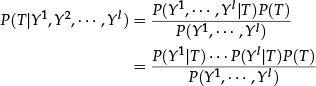
where the superscript on Y denotes the evidence order with a total of l number of evidences. This is also known as the naive Bayes classifier.

Suppose that among the total l measurements, there are l₀ number of Y₀ measurements, l₁ number of Y₁ measurements, and l₂ number of Y₂ measurements, i.e., l₀ + l₁ + l₂ = l. Substituting Eq. (1) and Eq. (7) yields,

$\begin{array}{ll}\hfill & P(T|Y_0^{1:l_0}\mathrm{,}{Y}_1^{1:l_1}\mathrm{,}{Y}_2^{1:l_2})=\frac{{\sigma }_0^{l_0}{\sigma }_{1T}^{l_1}{\sigma }_{2T}^{l_2}p}{{\sigma }_0^{l_0}{\sigma }_{1T}^{l_1}{\sigma }_{2T}^{l_2}p+{\sigma }_0^{l_0}{\sigma }_{1NT}^{l_1}{\sigma }_{2NT}^{l_2}(1-p)}.\hfill \end{array}$

(10)

2.4. Interaction between Subsystems

The agent comprises three subsystems: kinematics, informatics and classification. The kinematics subsystem describes the physical representation of the agent in the actual physical world that has several objects of interest in it. The important information that the agent gets from this subsystem is the relative distance, or the range, between the agent and the object of interest. In addition, the agent decides which direction to go in this subsystem, and the time history of these decisions creates the path of the agent. The informatics subsystem describes how the agent extracts information out of the object of interest. The extracted information is abstracted by three levels of measurement characteristics, denoted as Y₀, Y₁ and Y₂, that are distinguished qualitatively. Based on this information, the classification subsystem decides the property of the object of interest as being either a target or a non-target. The overview of the subsystem interconnection is shown in Fig. 2.

Figure 2.

Block diagram of interconnected subsystems

Kinematic decisions affect the classification result because the likelihood functions, Eq. (7), are dependent on the range between the agent and the object, and the posterior probability, Eq. (8), is a function of the likelihood functions. The classification results affect the kinematic decisions, i.e., if the agent classifies an object with high certainty it is likely that the agent will not approach the object closer, but seek a different object.

2.5. Strategy

In this section, we define the Bayes risk as the cost function for the dynamic optimization problem. First we define the confusion matrix, Which is shown in Table 2 (OOI: Object Of Interest). There are four possible outcomes.

Table 2.

Confusion matrix

	OOI in data	No OOI in data
Classifier says	OOI True Positive (TP)	False Positive (FP)
Classifier says no	OOI False Negative (FN)	True Negative (TN)

The probability and the loss function corresponding to each outcome are defined as P_outcome and L_outcome. Given the probabilities and the loss functions, one can define the risk function, R. The risk function takes two forms depending on the outcome of the random variable X. Let δ ∊ {NT, T} be the decision variable, then,

$R(X=NT\mathrm{,}\delta )=L_{TN}{P}_{TN}+L_{FP}{P}_{FP}$

(11a)

$R(X=T\mathrm{,}\delta )=L_{TP}{P}_{TP}+L_{FN}{P}_{FN}.$

(11b)

The first equation is the potential risk of making a decision when X = NT, while the second one is the case for X = T.

Without loss of generality, let L_TN = L_TF = 0 (i.e., there is no loss for correct decisions). Additionally, let

$P_{FP}=P(X=T|Y)$

(12a)

$P_{FN}=P(X=NT|Y)$

(12b)

Then the risk function takes the form of

$R(X=NT\mathrm{,}\delta |Y)=L_{FP}P(X=T|Y)$

(13a)

$R(X=T\mathrm{,}\delta |Y)=L_{FN}P(X=NT|Y)$

(13b)

This is called the conditional risk function. Note that the risk function varies depending on the type of observation, Y.

Bayes risk is the averaged risk function over the distribution of the random variables X and Y. Bayes risk with a single observation can be formulated as

$\begin{array}{ll}\hfill & R_B(\delta )=E_Y\left\{E_X\{R(X\mathrm{,}\delta |Y)\}\right\}\hfill \\ \hfill & ={\displaystyle \sum _{i=0}^2}\left\{P(NT)L_{FP}P(T|Y_i)+P(T)L_{FN}P(NT|Y_i)\right\}P(Y_i)\hfill \end{array}$

(14)

where R_B denotes Bayes risk and E_X denotes the expectation operator over random variable X. Note that the random variable representation in the probability mass function was omitted for the sake of simplicity, i.e., P(T) = P(X = T).

Loss Functions

In mission operations, the loss functions are determined by the strategist who decides the priority of the mission. There are several ways of posing the loss function. Depending on the loss function, the resultant paths are likely to be in one of two categories:

1. Strong emphasis on classified target being an actual target. In this case the loss function for false positive (FP), or false alarm, should be larger than the one for false negative (FN), i.e.,

   $L_{FP}\gg L_{FN}.$

   In summary, this is when the strategist places more emphasis on not judging non-targets as targets.

2. In the opposite situation, the emphasis is on the classified non-target being an actual non-target. In this case the loss function for false positive (FP), or false alarm, should be smaller than the one for false negative (FN), i.e.,

   $L_{FP}\ll L_{FN}.$

   In summary, this is when the strategist places more emphasis on not judging targets as non-targets.

3. Optimization Problem

We formulate the cost function, V, as the Bayes risk with two decision variables, φ (action) and δ (hypothesis). For one-stage optimization, V₁ = R_B(δ₁, φ₁), and V* = arg min _φ,δ V₁, where the subscript denotes the stage. SDP can be solved recursively using the optimality equation [19]. For M-stage optimization:

$V_M=\arg {\min }_{\varphi \mathrm{,}\delta }\left\{R_B({\delta }_1\mathrm{,}{\varphi }_1)+{\displaystyle \sum }{V}_{M-1}\right\}$

(15)

where M is the time constraint (mission time).

4. Stochastic Dynamic Programming

In the path planning, there are two decision problems at hand which are

• Whether to stay (and complete the mission) or to move (and take another observation).

We approach this decision problem with using the Bayes decision theory and solve it with stochastic dynamic optimization.

4.1. Decided to Stay

Suppose we are in the case where the agent decided to stay, i.e., φ = s. Now the agent faces a problem of deciding which hypothesis (X = T or X = NT) is true based on the up-to-date observations. In Bayes decision theory, this is formulated as the Bayes test for simple hypothesis [20]. Basically, the decision variable δ is a mapping between the observation set Y and the object property X, i.e., δ : Y → X. Let us define

$\begin{array}{c}{S}_{NT}=\{Y|\delta :Y\to NT\}\mathrm{,}\\ S_T=\{Y|\delta :Y\to T\}\mathrm{,}\end{array}$

with

$S_{NT}\cup S_T=Y,S_{NT}\cap S_T=\varnothing .$

Now the problem is to identify the sets S_NT and S_T. Reformulating the Bayes risk (Eq. (14)), it is given as (X and φ are omitted for notational simplicity)

$R_B(\delta \mathrm{,}Y)=P(NT)L_{FP}{P}_{FP}+P(T)L_{FN}{P}_{FN}.$

(16)

The probability of false positive and false negative can be defined with their probability distribution function. Let F(Y|X) be the probability distribution function of Y conditioned on X such that

${\displaystyle \sum _j^Y}F(Y_j|X)=P(Y|X).$

Then,

$\begin{array}{ll}{P}_{FP}\hfill & =P(\varphi (Y)=T|NT)\hfill \\ \hfill & =E_{NT}\{\varphi (Y)=T\}\hfill \\ \hfill & ={\displaystyle \sum _j^{S_T}}F(Y_j|NT)\hfill \end{array}$

(17)

and

$\begin{array}{ll}{P}_{FN}\hfill & =1-P(\varphi (Y)=T|T)\hfill \\ \hfill & =1-E_T\{\varphi (Y)=T\}\hfill \\ \hfill & =1-{\displaystyle \sum _j^{S_T}}F(Y_j|NT)\hfill \end{array}$

(18)

Substituting these into the Bayes risk formula gives

$\begin{array}{ll}\hfill & R_B(\delta \mathrm{,}Y)\hfill \\ =\hfill & P(T)L_{FN}+{\displaystyle \sum _j^{S_T}}\left[P(NT)L_{FP}F(Y_j|NT)-P(T)L_{FN}F(Y_j|T)\right].\hfill \end{array}$

(19)

Now using this formula, we want to find the set S_T. Suppose S_T = Ø, then

$R_B(\delta \mathrm{,}Y)=P(T)L_{FN}$

If there exists any Y that satisfies

$P(NT)L_{FP}F(Y_j|NT)<P(T)L_{FN}F(Y_j|T)$

the integrand in Eq. (19) will be negative, thus giving a smaller risk than P(T)L_FN. Rearranging the condition, we get

$\begin{array}{c}{S}_T=\left\{Y:\frac{F(Y_j|T)}{F(Y_j|NT)}>\frac{P(NT)L_{FP}}{P(T)L_{FN}}\right\}\mathrm{,}\\ S_{NT}=Y/S_T.\end{array}$

4.2. Decided to Move

The Bayes risk for the case where the agent decided to move is formulated as

$\begin{array}{ll}\hfill & R_B(\delta \mathrm{,}\varphi \ne s\mathrm{,}Y)\hfill \\ \hfill & =P(T)L_{FN}+\left\{P(NT)L_{FP}-P(T)L_{FN}\right\}P(T|Y).\hfill \end{array}$

(20)

The expected risk over the measurement Y is

$\begin{array}{ll}\hfill & R_B(\delta \mathrm{,}\varphi \ne s)=E_Y\left\{R_B(\delta \mathrm{,}\varphi \ne s\mathrm{,}Y)\right\}\hfill \\ \hfill & =P(T)L_{FN}+\left\{P(NT)L_{FP}-P(T)L_{FN}\right\}\hfill \\ \hfill & {\displaystyle \sum _{i=0}^2}P(Y_i|T)P(T)\hfill \\ \hfill & \hfill \end{array}$

(21)

where the second equation is obtained by using Bayes' theorem. There are four cases for the expected risk over the measurement, Y, each corresponding to different kinematic actions, i.e., φ = {u, d, l, r}.

4.2.1. Multiple Observations

The Bayes risk for multiple subsequent observations is formulated in this section. Here we introduce more notation: Ȳ is the sampled observation and the superscript indicates the sampled time instant. For instance,

${\bar{Y}}^{1:t}=\left[Y_1^1\mathrm{,}{Y}_0^2\mathrm{,}\cdots \mathrm{,}{Y}_2^t\right].$

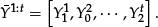
The Bayes risk of measurement at time t + 1 with sampled observation up to time t is

$\begin{array}{ll}\hfill & R_B(X\mathrm{,}\delta \mathrm{,}\varphi \ne s\mathrm{,}{\bar{Y}}^{1:t}\mathrm{,}{Y}^{t+1})=\hfill \\ \hfill & P(T)L_{FN}+\left\{P(NT)L_{FP}-P(T)L_{FN}\right\}P(T|{\bar{Y}}^{1:t}\mathrm{,}{Y}^{t+1})\hfill \end{array}$

(22)

Taking the expectation value over Y^t+1 yields

$\begin{array}{ll}\hfill & E_{Y^{t+1}}\left[R_B(X\mathrm{,}\delta \mathrm{,}\varphi \ne s\mathrm{,}{\bar{Y}}^{1:t}\mathrm{,}{Y}^{t+1})\right]=\hfill \\ \hfill & P(T)L_{FN}+\left\{P(NT)L_{FP}-P(T)L_{FN}\right\}\cdot \hfill \\ \hfill & \left\{{\displaystyle \sum _{i=0}^2}P(T|{\bar{Y}}^{1:t}\mathrm{,}{Y}_i^{t+1})P(Y_i^{t+1}|{\bar{Y}}^{1:t})\right\}\hfill \end{array}$

(23)

Since Y^1:t is conditionally independent of Y^t+1 given X, i.e., P(Y^t+1|T) = P(Y^t+1|T, Y^1:t), Bayes' theorem can be rewritten as

$\begin{array}{ll}P(T|{\bar{Y}}^{1:t}\mathrm{,}{Y}^{t+1})\hfill & =\frac{P(Y^{t+1}|T\mathrm{,}{\bar{Y}}^{1:t})P(T|{\bar{Y}}^{1:t})}{P(Y^{t+1}|{\bar{Y}}^{1:t})}\hfill \\ \hfill & =\frac{P(Y^{t+1}|T)P(T|{\bar{Y}}^{1:t})}{P(Y^{t+1}|{\bar{Y}}^{1:t})}.\hfill \end{array}$

(24)

Substituting this into the Bayes risk equation gives

$\begin{array}{ll}\hfill & E_{Y^{t+1}}\left[R_B(X\mathrm{,}\delta \mathrm{,}\varphi \ne s\mathrm{,}{\bar{Y}}^{1:t}\mathrm{,}{Y}^{t+1})\right]=\hfill \\ \hfill & P(T)L_{FN}+\left\{P(NT)L_{FP}-P(T)L_{FN}\right\}\cdot \hfill \\ \hfill & \left\{{\displaystyle \sum _{i=0}^2}P(Y_i^{t+1}|T)P(T|{\bar{Y}}^{1:t})\right\}.\hfill \end{array}$

(25)

This is the expected loss when the agent decides to move in some other direction. The actual risk may be larger or smaller depending on the sampled measurement. Supposing that we know the likelihood function, the risk can be determined.

5. Numerical Simulation Results

In this section, we present simulation results that were obtained by solving the SDP numerically. We used MATLAB as the simulation environment. First, we consider two scenarios, i.e., when L_FP > L_FN and when L_FP < L_FN, where an agent is to classify a single static object in a given area with non-informative prior (i.e., p = 0.5) as illustrated in Fig. 3 and Fig. 4. Then, we consider a scenario when targets appear very rarely (e.g., p = 0.001) with equal emphasis on the loss function (i.e., L_FP = L_FN) as shown in Fig. 5. Note that, considering the size of the search space, we have chosen the total mission time as M = 10.

Figure 3.

The resulting paths and the corresponding Bayes risk when L_FP is larger than L_FN (i.e., L_FP = 10, L_FN = 1) for p = 0.5 and ${\theta }_{Y_1|X}={\theta }_{Y_2|X}=\pi$

Figure 4.

The resulting paths and the corresponding Bayes risk when L_FP is smaller than L_FN (i.e., L_FP = 1, L_FN = 10) for p = 0.5 and ${\theta }_{Y_1|X}={\theta }_{Y_2|X}=\pi$

Figure 5.

The resulting paths and the corresponding Bayes risk when L_FP is equal to L_FN (i.e., L_FP = 10, L_FN = 10) for p = 0.001 and ${\theta }_{Y_1|X}={\theta }_{Y_2|X}=\pi$

Figure 3(a) shows the agent movement in a 2-D space for four different initial positions each of which is colour-coded. The loss functions are L_FP = 10 and L_FN = 1 such that L_FP > L_FN, i.e., the strategist places more emphasis on not judging non-targets as targets. The black square and the black star correspond to the initial and ending position, respectively. When the loss is higher for FP than FN, the agent decides to move towards the object for better observations as shown. Regardless of the initial positions, the agent first moves closer to the object, then converges to the vantage point of the object, as indicated by a dashed box. Figure 3(b) shows the corresponding Bayes risk as a function of the time step. Note that the risk for staying (dashed lines) is always greater than the risk for moving (dash dot lines) in this particular scenario, so the agent stops when the total mission time is reached. It should also be noted that as the agent enters the vantage points of the object, it moves back and forth between the alternate locations among the vantage points. This is a consequence of the fact that the minimal risk is reached before the mission time is completed and the minimal solution is non-unique. This suggests that additional stopping criteria may be needed when there is no improvement in the risk, such that the agent need not waste time on the given object. This may not be a problem, however, when there are multiple objects with a stringent time constraint, as the agent will run out of time before examining all the objects.

Figure 4(a) shows the agent movement for four same initial positions as in Fig. 3(a), but with the loss functions being L_FP = 1 and L_FN = 10 such that L_FP < L_FN, i.e., the strategist places more emphasis on not judging targets as non-targets. Note that the scale of the axes is different from that of Fig. 3(a). In contrast to the previous case, the agent moves away from the object and it decides to stay at a few time steps, except for the case that starts at a poor vantage (blue line). Figure 4(b) shows the corresponding Bayes risk as a function of the time step.

Figure 5(a) shows the agent movement with the loss functions being L_FP = 10 and L_FN = 10 such that L_FP = L_FN, i.e., the strategist places no particular emphasis on either outcome, and the prior probability is extremely small, i.e., p = 0.001. Note that in actual ISR scenarios, the number of targets is considerably smaller than the number of non-targets, which corresponds to a small value of p. Regardless of the initial position, the agent terminates its exploration at the second time step, as shown in the figure. This is because the prior probability is extremely small and no particular emphasis was made in the loss function by the strategist, which discourages further investigation as there is no incentive. Figure 5(b) shows the corresponding Bayes risk as a function of the time step.

6. Conclusion & Future Work

In this paper, we proposed a model that accounts for the interaction between the agent kinematics, informatics, classification and strategy. For kinematics, the agent follows the Manhattan gridded space where there are five kinematic decisions that correspond to the directions of movement (i.e., up, down, left, right) and stay. For informatics, the measurement is abstracted by three discrete measurement types (i.e., Y₀, Y₁ and Y₂ depending on the quality) where each measurement type has its own likelihood function that follows the modified performance prediction model (MPPM). For classification, the agent follows the Bayes inference with an assumption that subsequent measurements are conditionally independent given the object category. For strategy, we use the Bayes risk formulation (i.e., the expected loss over the distribution of the random variables X and Y) whose loss functions are determined by the strategist who dictates the priority of the mission. Within this model, we pose and solve a sequential decision problem whose objective is to minimize the Bayes risk over a given mission time. The solution of the sequential decision problem yields the following flying tactics: “approach only objects whose suspected identity matters to the strategy”. These tactics are numerically illustrated in several scenarios.

As future work, we will investigate several avenues which are 1. inclusion of the azimuth-dependent measurement model, 2. online estimation of the likelihood function, and 3. mathematical definition of target “deception”. Furthermore, we plan to investigate the effects of couplings between different subsystems (e.g., classification and strategy), as well as objective functions (e.g., information and classification performance), in path planning applications.