Analytical model for investigation of the effect of friction power on temperature in the disk brake

Abstract

In this article, the effect of different time profiles of friction power on a temperature distribution in friction element of a brake has been analyzed. For this purpose, a one-dimensional heat problem of friction during braking for 10 temporal profiles of the specific power of friction has been formulated and solved exactly. Based on the analytical solutions, numerical calculations of the temperature distributions have been carried out. A comparative analysis of the obtained results with corresponding data, that were found using an approximate solution from the Chichinadze’s monograph titled Calculation and study of external friction during braking, has also been performed. Conducted numerical analysis has allowed us to establish the applicability limits of this approximate solution. We also determined that the temporal profile of friction power has a significant influence on the evolution of the surface temperature, and on temperature field inside a disk brake.

Introduction

The intensity of the heat flux at the contact region on the friction surface is determined in advance and usually in a form of a linearly decreasing function of time $t$ ^1–4 in most of the calculation models determining temperature fields during braking. It means that the product of friction coefficient $f(t)$ and contact pressure $p(t)$ is assumed to be constant, that is, $f(t)p(t)=\mathrm{const}$ . In addition, it is assumed that the load on a nominal area of contact increases rapidly with the beginning of a braking process to a nominal value. This assumption reduces the reliability of the simulation. In fact, temporal profile of the heat flux intensity, which is proportional to a specific power of friction $q(t)=f(t)p(t)V(t)$ , can be significantly different from the linear one.^5,6 Analytical solutions to the one-dimensional thermal problems of friction with account of time-dependent increase in contact pressure have been obtained in some of the papers.^7–10 Analytical models of frictional heating with three different heat fluxes, for a homogeneous semi-space, which simulates a disk brake, have been proposed in the article by Topczewska. ¹¹ Solution to the heat conduction problem for two semi-infinite solids with account of change in the friction coefficient under the influence of the temperature has been received in the article by Olesiak et al. ¹² Consideration of thermosensitivity of materials and their mutual dependence of temperature on the contact surface and the friction coefficient in a tribosystem consisting of two semi-spaces has been conducted in the paper by Yevtushenko et al. ¹³ Extensive review of developed one-dimensional analytical models of frictional heating has been explained in the article by Yevtushenko and Kuciej. ¹⁴

In this work, it has been established that there is a lack of exact solutions to these problems, which considered more complex temporal profile of friction power. However, such an approximate solution, which allows to perform temperature calculations for any profile of friction power, has been obtained in the monograph. ¹⁵ In this article, a classification of temporal profile of the specific power of friction, characteristic for various braking modes, has been carried out.

The aim of this article is to obtain exact solutions to one-dimensional thermal problem of friction during single braking, for the above-mentioned profiles of the specific power of friction, and to compare data with the relevant results obtained by means of an approximate solution from Chichinadze’s monograph. ¹⁵

Temporal profile of the specific power of friction and the work of braking

Characteristics of friction and wear of braking system elements may considerably vary depending on the manner in which this system absorbs braking energy. There are various cases possible: in some, a significant part of braking energy is realized in an initial period of the process, and in others, braking work is distributed more uniformly over time. The time profile of friction power determines temporal profiles of braking work. This profile is the main factor responsible for the following: spatio-temporal distributions of temperature in friction elements, the maximum temperature, and its gradient along the normal to the friction surface. ¹⁶

The list of 10 functions that describes the change in the specific power of friction with time $t$ during single braking

$$q_i(t)=q_0{q}_i^{*}(t),0\le t\le t_s,i=1,2,...,10$$

(1)

has been presented in the monograph. ¹⁵ Where $q_0$ is the nominal value of specific power of friction and $q_i^{*}(t)$ are dimensionless profiles of specific power of friction (Table 1).

Table 1.

Dimensionless specific power of friction $q_i^{*}(t)$ with the maximal values $q_{i,max}^{*}$ achieved at the moment of time $t_{i,max}$ and the dimensionless density of the braking work $w_i^{*}(t)$ , $i=1,2,...,10$ .

$i$	$q_i^{*}(t)$	$q_{i,max}^{*}$	$t_{i,max}$	$w_i^{*}(t)$
1	$2(1-t^{*})$	2	0	$t^{*}(2-t^{*})$
2	$2t^{*}$	2	$t_s$	$t^{{*}^2}$
3	$\frac{3}{2}\sqrt{1-t^{*}}$	1.5	0	$1-(1-t^{*})\sqrt{1-t^{*}}$
4	$\frac{3}{2}\sqrt{t^{*}}$	1.5	$t_s$	$t^{*}\sqrt{t^{*}}$
5	$3(1-t^{*}{)}^2$	3	0	$3t^{*}(1-t^{*}+\frac{1}{3}{t}^{{*}^2})$
6	$3t^{{*}^2}$	3	$t_s$	$t^{{*}^3}$
7	$6t^{*}(1-t^{*})$	1.5	0.5 $t_s$	$t^{{*}^2}(3-2t^{*})$
8	$\frac{6}{5}(1-t^{*})(1+2t^{*})$	1.35	0.25 $t_s$	$\frac{6}{5}{t}^{*}(1+\frac{1}{2}{t}^{*}-\frac{2}{3}{t}^{{*}^2})$
9	$\frac{18}{5}{t}^{*}(1-\frac{2}{3}{t}^{*})$	1.35	0.75 $t_s$	$\frac{1}{5}{t}^{{*}^2}(9-4t^{*})$
10	$6\sqrt{t^{*}}(1-\sqrt{t^{*}})$	1.5	0.25 $t_s$	$t^{*}\sqrt{t^{*}}(4-3\sqrt{t^{*}})$

Taking into account formula (1), the density of work executed by a friction pair in the braking process is equal to

$$w_i(t)\equiv \underset{0}{\overset{t}{\int }}{q}_i(s)\mathrm{ds}=w_0{w}_i^{*}(t),0\le t\le t_s,i=1,2,...,10$$

(2)

where

$$w_0=q_0{t}_s,w_i^{*}(t)=t_s^{-1}\underset{0}{\overset{t}{\int }}{q}_i^{*}(s)\mathrm{ds}$$

(3)

From formulas (2) and (3), the total density of work, which was made by friction couple during a single braking process, was found in the form

$$w_i(t_s)=w_0{w}_i^{*}(t_s),i=1,2,...,10$$

(4)

In order to perform a comparative analysis of the influence of all 10 time profiles (1) on the temperature distribution in the friction element of brake, we will examine the processes with the same braking work at the same braking time $t=t_s$ , that is

$$w_i^{*}(t_s)=1,i=1,2,...,10$$

(5)

The list of dimensionless functions $q_i^{*}(t)$ (1) and $w_i^{*}(t)$ , $i=1,2,...,10$ (3) from the monograph, ¹⁵ that satisfies condition (5), is given in Table 1 and their graphs are shown in Figures 1 and 2, respectively. The values of the maximum specific power of friction $q_{i,max}^{*}$ , $i=1,2,...,10$ and time to achieve them $t_{i,max}$ is also shown in Table 1.

Figure 1.

Scheme of the problem.

Figure 2.

Evolution of dimensionless specific power of friction $q_i^{*}(t)$ : (a) $i=1,2,...,6$ and (b) $i=7,8,910$ .

Statement of the one-dimensional heat problem of friction during braking

During unforced cooling of friction elements in braking system, the range of heat transfer coefficient value is typically equal to $h=20-60$ W/(m²°C).^17,18 It has been found that such values do not significantly affect surface temperature during processes with the Fourier number ${\tau }_s=k{t}_s/a^2\le 10$ . ¹⁹ The effective depth of heat penetration (the depth from heated surface, on which achieved temperature has value equal to the 5% of the maximum temperature on this surface) during braking is equal to $a=\sqrt{3k{t}_s}$ , ¹⁵ and then the typical value ${\tau }_s\cong 0.33$ . Thus, in statement of the one-dimensional thermal problems of friction, it is assumed that the free surfaces of element are adiabatic.

The next simplifying assumption in mathematical modeling of frictional heating process takes into account an experimentally determined result, that the largest part of heat generated on the friction surface is absorbed by sliding elements in a direction perpendicular to this surface. ²⁰ Thus, in the heat conduction equations, we can neglect the changes in temperature gradients in radial and circumferential directions.

One of the approaches to formulate thermal problems of friction during braking is based on a virtual separation of friction pair elements (e.g. a pad and a disk) and heating their working surfaces by the heat fluxes with the intensity proportional to the power of friction. ¹⁴ As the coefficient of proportionality, there is a so-called coefficient of heat partition ratio. This coefficient is determined using the empirical formula^21,22 established on the basis of experimental investigations. It is chosen in such a way that a sum of intensities of the heat fluxes, directed along to the normal to the friction surface, is equal to the specific power of friction. Usually, it is assumed that the value of the heat partition ratio is equal to 1.

At the initial time moment $t=0$ , a considered element of friction pair is uniformly heated to the ambient temperature $T_a$ .

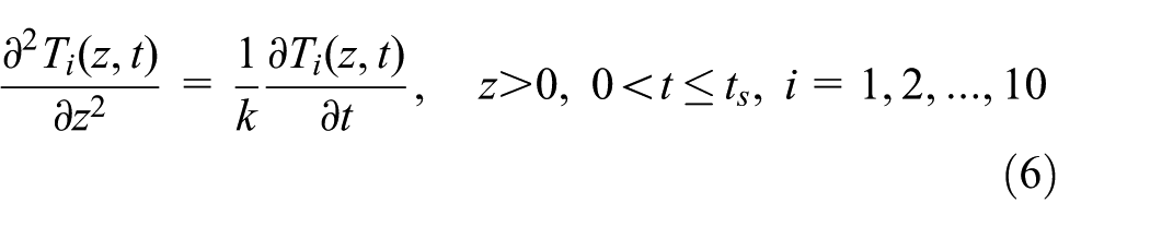
Taking into account the above-mentioned assumptions, the temperature fields $T_i$ , initiated by heating the surface $z=0$ of the semi-infinity body $z\ge 0$ (Figure 1) by heat fluxes with intensities $q_i$ , $i=1,2,...,10$ (1), were found from the solution of the following one-dimensional thermal problem of friction during braking

$$\frac{{\partial }^2{T}_i(z,t)}{\partial z^2}=\frac{1}{k}\frac{\partial T_i(z,t)}{\partial t},z>0,0<t\le t_s,i=1,2,...,10$$

(6)

$${K\frac{\partial T_i(z,t)}{\partial z}|}_{z=0}=-q_i(t),0<t\le t_s,i=1,2,...,10$$

(7)

$$T_i(z,t)\to 0,z\to \infty ,0<t\le t_s,i=1,2,...,10$$

(8)

$$T_i(z,0)=T_a,z\ge 0,i=1,2,...,10$$

(9)

where $k$ is the thermal diffusivity and $K$ is the thermal conductivity.

Introducing the following dimensionless variables and parameters

$$\zeta =\frac{z}{a},\tau =\frac{\mathrm{kt}}{a^2},T_i^{*}=\frac{T_i-T_a}{T_0},T_0=\frac{w_{0}a}{t_{s}K}$$

(10)

The boundary-value problem of heat conduction (6)–(9) was written in the dimensionless form

$$\frac{{\partial }^2{T}_i^{*}(\zeta ,\tau )}{\partial {\zeta }^2}=\frac{\partial T_i^{*}(\zeta ,\tau )}{\partial \tau },\zeta >0,0<\tau \le {\tau }_s,i=1,2,...,10$$

(11)

$${\frac{\partial T_i^{*}(\zeta ,\tau )}{\partial \zeta }|}_{\zeta =0}=-q_i^{*}(\tau ),0<\tau \le {\tau }_s,i=1,2,...,10$$

(12)

$$T_i^{*}(\zeta ,\tau )\to 0,\zeta \to \infty ,0<\tau \le {\tau }_s,i=1,2,...,10$$

(13)

$$T_i^{*}(\zeta ,0)=0,\zeta \ge 0,i=1,2,...,10$$

(14)

and forms of the functions $q_i^{*}(t)$ , $i=1,2,...,10$ in the right side of the boundary condition (12) are presented in Table 1.

Exact solution to the problem

The solution of the boundary-value problem of heat conductivity (11)–(14) was found using the Duhamel’s formula ²³

$$\begin{array}{l}{T}_i^{\ast }(\zeta ,\tau )=\\ {\displaystyle \underset{0}{\overset{\tau }{\int }}{q}_i^{\ast }(s)\frac{\partial }{\partial \tau }}{T}_0^{\ast }(\zeta ,\tau -s)ds,\zeta \ge 0,0\le \tau \le {\tau }_s,i=1,2,\dots ,10\end{array}$$

(15)

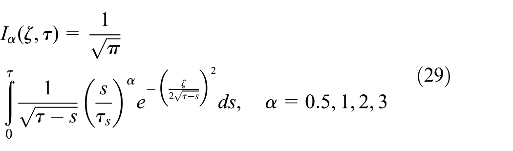
where

$$T_0^{*}(\zeta ,\tau )=2\sqrt{\tau }\mathrm{ierfc}Z,\zeta \ge 0,0\le \tau \le {\tau }_s$$

(16)

$$Z=0.5\zeta /\sqrt{\tau }$$

(17)

is the known solution to the above-mentioned problem (11)–(14) with the function $q_0^{*}(\tau )=1$ in the right side of the boundary condition (12). ⁵

Taking into account a derivative ²⁴

$$\frac{\partial }{\partial \tau }\left[2\sqrt{\tau -s}\mathrm{ierfc}\left(\frac{\zeta }{2\sqrt{\tau -s}}\right)\right]=\frac{e^{-{\left(\frac{\zeta }{2\sqrt{\tau -s}}\right)}^2}}{\sqrt{\pi (\tau -s)}}$$

(18)

the dimensionless temperature $T_i^{*}(\zeta ,\tau )$ , $\zeta \ge 0,0\le \tau$ , $\le {\tau }_s$ , $i=1,2,...,10$ (15)–(17) was written in the following form

$$T_1^{*}(\zeta ,\tau )=2[T_0^{*}(\zeta ,\tau )-I_1(\zeta ,\tau )]$$

(19)

$$T_2^{*}(\zeta ,\tau )=2I_1(\zeta ,\tau )$$

(20)

$$T_3^{*}(\zeta ,\tau )=\frac{3}{2}[T_0^{*}(\zeta ,\tau )-\frac{1}{2}{I}_1(\zeta ,\tau )-\frac{1}{8}{I}_2(\zeta ,\tau )-\frac{1}{16}{I}_3(\zeta ,\tau )]$$

(21)

$$T_4^{*}(\zeta ,\tau )=\frac{3}{2}{I}_{0.5}(\zeta ,\tau )$$

(22)

$$T_5^{*}(\zeta ,\tau )=3[T_0^{*}(\zeta ,\tau )-2I_1(\zeta ,\tau )+I_2(\zeta ,\tau )]$$

(23)

$$T_6^{*}(\zeta ,\tau )=3I_2(\zeta ,\tau )$$

(24)

$$T_7^{*}(\zeta ,\tau )=6[I_1(\zeta ,\tau )-I_2(\zeta ,\tau )]$$

(25)

$$T_8^{*}(\zeta ,\tau )=\frac{6}{5}[T_0^{*}(\zeta ,\tau )+I_1(\zeta ,\tau )-2I_2(\zeta ,\tau )]$$

(26)

$$T_9^{*}(\zeta ,\tau )=\frac{18}{5}[I_1(\zeta ,\tau )-\frac{2}{3}{I}_2(\zeta ,\tau )]$$

(27)

$$T_{10}^{*}(\zeta ,\tau )=6[I_{0.5}(\zeta ,\tau )-I_1(\zeta ,\tau )]$$

(28)

where

$$\begin{array}{l}{I}_{\alpha }(\zeta ,\tau )=\frac{1}{\sqrt{\pi }}\\ {\displaystyle \underset{0}{\overset{\tau }{\int }}\frac{1}{\sqrt{\tau -s}}{\left(\frac{s}{{\tau }_s}\right)}^{\alpha }{e}^{-{\left(\frac{\zeta }{2\sqrt{\tau -s}}\right)}^2}}ds,\alpha =0.5,1,2,3\end{array}$$

(29)

It should be noted that at determining the dimensionless temperature $T_3^{*}(\zeta ,\tau )$ (21), we used the expansion of the function $q_3^{*}(\tau )$ in the form of the power series

$$q_3^{*}(\tau )=\frac{3}{2}[1-\frac{1}{2}\left(\frac{\tau }{{\tau }_s}\right)-\frac{1}{8}{\left(\frac{\tau }{{\tau }_s}\right)}^2-\frac{1}{16}{\left(\frac{\tau }{{\tau }_s}\right)}^3+\cdots ]$$

(30)

with the subsequent restriction in it the first four components.

Using the substitution $x=1/\sqrt{\tau -s}$ , the integrals $I_{\alpha }(\zeta ,\tau )$ , $\alpha =0.5,1,2,3$ (29) were presented in the following form

$$I_{0.5}(\zeta ,\tau )=\sqrt{\frac{\tau }{{\tau }_s\pi }}J(\zeta ,\tau )$$

(31)

$$I_1(\zeta ,\tau )=\frac{2}{{\tau }_s\sqrt{\pi }}[\tau J_2(\zeta ,\tau )-J_4(\zeta ,\tau )]$$

(32)

$$I_2(\zeta ,\tau )=\frac{2}{{\tau }_s^2\sqrt{\pi }}[{\tau }^2{J}_2(\zeta ,\tau )-2\tau J_4(\zeta ,\tau )+J_6(\zeta ,\tau )]$$

(33)

$$\begin{array}{l}{I}_3(\zeta ,\tau )=\frac{2}{{\tau }_s^3\sqrt{\pi }}\\ [{\tau }^3{J}_2(\zeta ,\tau )-3{\tau }^2{J}_4(\zeta ,\tau )+3\tau J_6(\zeta ,\tau )-J_8(\zeta ,\tau )]\end{array}$$

(34)

where

$$J(\zeta ,\tau )=\underset{{\tau }^{-1}}{\overset{\infty }{\int }}{x}^{-2}\sqrt{x-{\tau }^{-1}}{e}^{-{(0.5\zeta )}^{2}x}\mathrm{dx}$$

(35)

$$J_k(\zeta ,\tau )=\underset{1/\sqrt{\tau }}{\overset{\infty }{\int }}{x}^{-k}{e}^{-{(0.5\zeta )}^{2}x}\mathrm{dx},k=2,4,6,8$$

(36)

Integrating by parts in the right side of equation (35), we obtained

$$J(\zeta ,\tau )=0.5J_0(\zeta ,\tau )-0.25{\zeta }^2{J}_1(\zeta ,\tau )$$

(37)

where

$$J_k(\zeta ,\tau )=\underset{{\tau }^{-1}}{\overset{\infty }{\int }}{x}^{-1}{(x-{\tau }^{-1})}^{k-1/2}{e}^{-{(0.5\zeta )}^{2}x}\mathrm{dx},k=0,1$$

(38)

Using the formula ²⁵

$$\underset{u}{\overset{\infty }{\int }}{x}^{-1}{(x-u)}^{\nu }{e}^{-\mu x}\mathrm{dx}=u^{\nu }\mathrm{\Gamma }(\nu +1)\mathrm{\Gamma }(-\nu ,u\mu ),u>0,\mathrm{Re}\nu >-1,\mathrm{Re}\mu >0$$

(39)

the integrals (38) were written in the form

$$J_k(\zeta ,\tau )={\tau }^{1/2-k}\mathrm{\Gamma }(0.5+k)\mathrm{\Gamma }(0.5-k,Z^2),k=0,1$$

(40)

where a generalized variable $Z$ has the form (17). Taking into account values of gamma function

$$\mathrm{\Gamma }(0.5)=\sqrt{\pi },\mathrm{\Gamma }(1.5)=0.5\sqrt{\pi }$$

(41)

and an incomplete gamma function ²⁴

$$\mathrm{\Gamma }(0.5,Z^2)=\sqrt{\pi }\mathrm{erfc}Z,\mathrm{\Gamma }(-0.5,Z^2)=2\sqrt{\pi }{Z}^{-1}\mathrm{ierfc}\mathrm{Z}$$

(42)

from formulas (40), the following was found

$$J_0(\zeta ,\tau )=\pi \sqrt{\tau }\mathrm{erfc}\mathrm{Z},J_1(\zeta ,\tau )=\frac{\pi }{Z\sqrt{\tau }}\mathrm{ierfc}\mathrm{Z}$$

(43)

Substituting the function $J_k(\zeta ,\tau )$ , $k=0,1$ to the right side of equation (40), we received

$$J(\zeta ,\tau )=0.5\pi \sqrt{\tau }(\mathrm{erfc}Z-2Z\mathrm{ierfc}Z)$$

(44)

Taking into account the form of the function $J(\zeta ,\tau )$ (44), we found from formula (31)

$$I_{0.5}(\zeta ,\tau )=0.5\sqrt{\pi {\tau }_s}{\tau }^{*}(\mathrm{erfc}\mathrm{Z}-2Z\mathrm{ierfc}Z),{\tau }^{*}=\tau /{\tau }_s$$

(45)

Integrals (36) for $k=4,6,8$ , we calculated using a recursive formula

$$J_k(\zeta ,\tau )=\frac{\sqrt{{\tau }^{k-1}}}{(k-1)}{e}^{-Z2}-\frac{{\zeta }^2}{2(k-1)}{L}_{k-2}(\zeta ,\tau )$$

(46)

where ²⁵

$$J_2(\zeta ,\tau )=\sqrt{\pi \tau }\mathrm{ierfc}Z$$

(47)

As a result, the following were obtained

$$J_4(\zeta ,\tau )=\frac{1}{3}\tau \sqrt{\pi \tau }[(1-2Z^2)\mathrm{ierfc}Z+Z\mathrm{erfc}Z]$$

(48)

$$\begin{array}{l}{J}_6(\zeta ,\tau )=\frac{1}{15}{\tau }^2\sqrt{\pi \tau }\\ \{[3-2Z^2(1-2Z^2)]\mathrm{ierfc}Z+Z(3-2Z^2)\mathrm{erfc}Z\}\end{array}$$

(49)

$$\begin{array}{l}{J}_8(\zeta ,\tau )=\frac{1}{105}{\tau }^3\sqrt{\pi \tau }\\ [(15-6Z^2+4Z^4-8Z^6)\mathrm{ierfc}Z+Z(15-6Z^2+4Z^4)\mathrm{erfc}Z]\end{array}$$

(50)

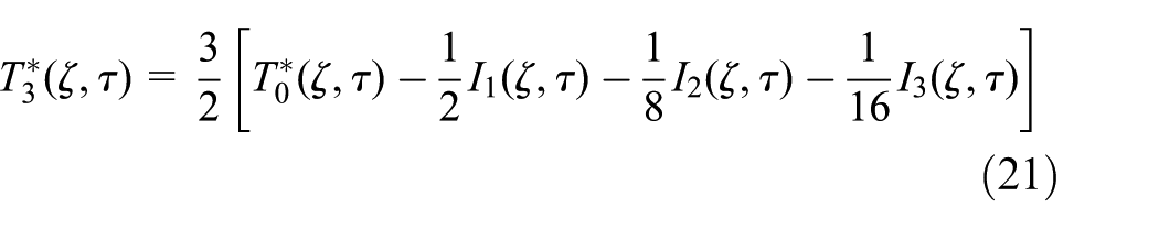
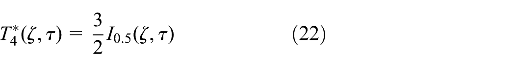
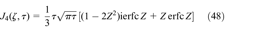
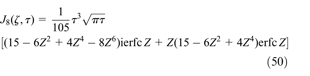
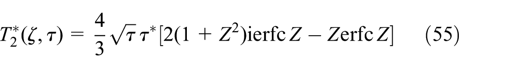
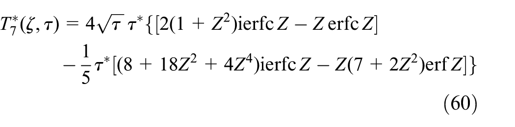
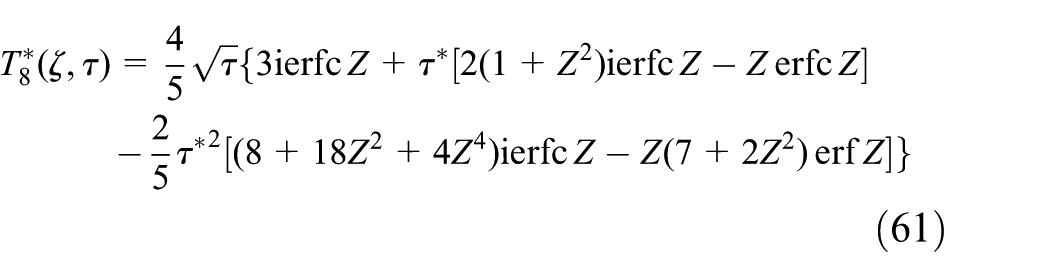
Substituting functions $J_k(\zeta ,\tau )$ (48)–(50) into formulae (32)–(34), we received

$$I_1(\zeta ,\tau )=\frac{2}{3}\sqrt{\tau }{\tau }^{*}[2(1+Z^2)\mathrm{ierfc}Z-Z\mathrm{erfc}Z]$$

(51)

$$\begin{array}{l}{I}_2(\zeta ,\tau )=\frac{2}{15}\sqrt{\tau }{\tau }^{\ast 2}\\ [(8+18Z^2+4Z^4)\mathrm{ierfc}Z-Z(7+2Z^2)\mathrm{erfc}Z]\end{array}$$

(52)

$$\begin{array}{l}{I}_3(\zeta ,\tau )=\frac{2}{105}\sqrt{\tau }{\tau }^{\ast 3}\\ [(48+174Z^2+80Z^4+8Z^6)\mathrm{ierfc}Z-Z(57+36Z^2+4Z^4)\mathrm{erfc}Z]\end{array}$$

(53)

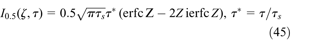
Substituting the functions $I_{\alpha }(\zeta ,\tau )$ , $\alpha =0.5,1,2,3$ (45), (51)–(53) into formulae (19)–(28), we found a dimensionless temperature fields $T_i^{*}(\zeta ,\tau )$ , $\zeta \ge 0$ , $0\le \tau \le {\tau }_s$ , $i=1,2,...,10$ in the forms

$$T_1^{*}(\zeta ,\tau )=\frac{4}{3}\sqrt{\tau }{\tau }^{*}\{[3{{\tau }^{*}}^{-1}-2(1+Z^2)]\mathrm{ierfc}Z+Z\mathrm{erfc}Z\}$$

(54)

$$T_2^{*}(\zeta ,\tau )=\frac{4}{3}\sqrt{\tau }{\tau }^{*}[2(1+Z^2)\mathrm{ierfc}Z-Z\mathrm{erfc}Z]$$

(55)

$$\begin{array}{c}{T}_3^{*}(\zeta ,\tau )=3\sqrt{\tau }\mathrm{ierfc}Z-\frac{1}{2}\sqrt{\tau }{\tau }^{*}[2(1+Z^2)\mathrm{ierfc}Z-Z\mathrm{erfc}Z]\hfill \\ -\frac{1}{40}\sqrt{\tau }{{\tau }^{*}}^2[(8+18Z^2+4Z^4)\mathrm{ierfc}Z-Z(7+2Z^2)\mathrm{erfc}Z]\hfill \\ -\frac{1}{560}\sqrt{\tau }{{\tau }^{*}}^3[(48+174Z^2+80Z^4+8Z^6)\mathrm{ierfc}Z-Z(57+36Z^2+4Z^4)\mathrm{erfc}Z]\hfill \end{array}$$

(56)

$$T_4^{*}(\zeta ,\tau )=\frac{3}{4}\sqrt{\pi {\tau }_s}{\tau }^{*}[\mathrm{erfc}Z-2Z\mathrm{ierfc}Z]$$

(57)

$$\begin{array}{c}{T}_5^{*}(\zeta ,\tau )=2\sqrt{\tau }\{3\mathrm{ierfc}Z-2{\tau }^{*}[2(1+Z^2)\mathrm{ierfc}Z-Z\mathrm{erfc}Z]\hfill \\ +\frac{1}{5}{{\tau }^{*}}^2[(8+18Z^2+4Z^4)\mathrm{ierfc}Z-Z(7+2Z^2)\mathrm{erfc}Z]\}\hfill \end{array}$$

(58)

$$T_6^{*}(\zeta ,\tau )=\frac{2}{5}\sqrt{\tau }{{\tau }^{*}}^2[(8+18Z^2+4Z^4)\mathrm{ierfc}Z-Z(7+2Z^2)\mathrm{erfc}Z]$$

(59)

$$\begin{array}{c}{T}_7^{*}(\zeta ,\tau )=4\sqrt{\tau }{\tau }^{*}\{[2(1+Z^2)\mathrm{ierfc}Z-Z\mathrm{erfc}Z]\hfill \\ -\frac{1}{5}{\tau }^{*}[(8+18Z^2+4Z^4)\mathrm{ierfc}Z-Z(7+2Z^2)\mathrm{erf}Z]\}\hfill \end{array}$$

(60)

$$\begin{array}{c}{T}_8^{*}(\zeta ,\tau )=\frac{4}{5}\sqrt{\tau }\{3\mathrm{ierfc}Z+{\tau }^{*}[2(1+Z^2)\mathrm{ierfc}Z-Z\mathrm{erfc}Z]\hfill \\ -\frac{2}{5}{{\tau }^{*}}^2[(8+18Z^2+4Z^4)\mathrm{ierfc}Z-Z(7+2Z^2)\mathrm{erf}Z]\}\hfill \end{array}$$

(61)

$$\begin{array}{c}{T}_9^{*}(\zeta ,\tau )=\frac{4}{5}\sqrt{\tau }{\tau }^{*}\{3[2(1+Z^2)\mathrm{ierfc}Z-Z\mathrm{erfc}Z]-\hfill \\ -\frac{2}{5}{\tau }^{*}[(8+18Z^2+4Z^4)\mathrm{ierfc}Z-Z(7+2Z^2)\mathrm{erf}Z]\}\hfill \end{array}$$

(62)

$$\begin{array}{l}{T}_{10}^{\ast }(\zeta ,\tau )={\tau }^{\ast }\{3\sqrt{\pi {\tau }_s}(\mathrm{erfc}Z-2Z\mathrm{ierfc}Z)\\ -4\sqrt{\tau }[2(1+Z^2)\mathrm{ierfc}Z-Z\mathrm{erfc}Z]\}\end{array}$$

(63)

where the dimensionless parameters $Z$ and ${\tau }^{*}$ have the form (17) and (45), respectively.

Approximate Chichinadze’s solution

The approximate Chichinadze’s solution has been obtained in the monograph, ¹⁵ and it can still be used to calculate the temperature of the brake systems.^26,27 This solution is little known in English-language scientific literature; therefore, we allow ourselves to present the main steps of obtaining it.

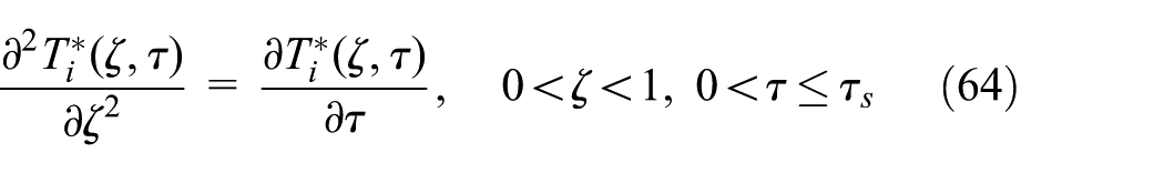
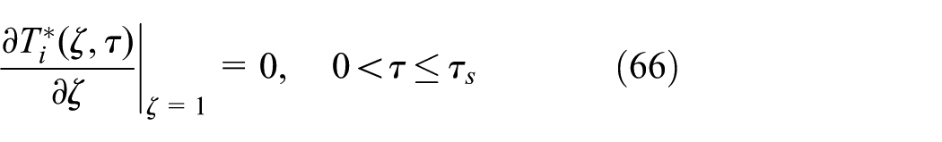
Let a homogeneous strip $0\le z\le a$ be heated on the surface $z=0$ by heat flux with the time-dependent intensity $q_i(t)$ , $0\le t\le t_s$ , $i=1,2,...,10$ and surface $z=a$ is adiabatic. At the initial time moment $t=0$ , the temperature of the strip is equal to the ambient temperature $T_a$ . Taking into account indications (10) of the transient distribution of the dimensionless temperature $T_i^{*}(\zeta ,\tau )$ , $i=1,2,...,10$ , in the strip, we find the solution to the following boundary-value heat conduction problem

$$\frac{{\partial }^2{T}_i^{*}(\zeta ,\tau )}{\partial {\zeta }^2}=\frac{\partial T_i^{*}(\zeta ,\tau )}{\partial \tau },0<\zeta <1,0<\tau \le {\tau }_s$$

(64)

$${\frac{\partial T_i^{*}(\zeta ,\tau )}{\partial \zeta }|}_{\zeta =0}=-q_i^{*}(\tau ),0<\tau \le {\tau }_s$$

(65)

$${\frac{\partial T_i^{*}(\zeta ,\tau )}{\partial \zeta }|}_{\zeta =1}=0,0<\tau \le {\tau }_s$$

(66)

$$T_i^{*}(\zeta ,0)=0,0\le \zeta \le 1$$

(67)

where dimensionless forms of the specific power of friction $q_i^{*}(t)$ are presented in Table 1.

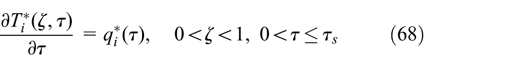
The main idea of Chichinadze was to find a convenient solution to the problem (64)–(67) for any temporal profile of specific friction power in a form that would be useful in numerical analysis. ¹⁵ To obtain this comprehensive solution, it has been assumed additionally that a change in temperature with time at any point in the strip is proportional to the specific power of friction

$$\frac{\partial T_i^{*}(\zeta ,\tau )}{\partial \tau }=q_i^{*}(\tau ),0<\zeta <1,0<\tau \le {\tau }_s$$

(68)

Taking into account the assumption (68) in equation (64), we achieved

$$\frac{{\partial }^2{T}_i^{*}(\zeta ,\tau )}{\partial {\zeta }^2}=q_i^{*}(\tau ),0<\tau \le {\tau }_s$$

(69)

Integrating equation (69) with respect to the spatial coordinate $\zeta$ , we obtained

$$\frac{\partial T_i^{*}(\zeta ,\tau )}{\partial \zeta }=\zeta q_i^{*}(\tau )+C_1(\tau ),0<\zeta <1,0<\tau \le {\tau }_s$$

(70)

where unknown function $C_1(\tau )$ was determined from the boundary condition (65)

$$C_1(\tau )=-q_i^{*}(\tau ),0<\tau \le {\tau }_s$$

(71)

Substituting the function $C_1(\tau )$ (71) to the right side of equation (70), we found

$$\frac{\partial T_i^{*}(\zeta ,\tau )}{\partial \zeta }=(\zeta -1)q_i^{*}(\tau ),0\le \zeta \le 1,0<\tau \le {\tau }_s$$

(72)

Let us note that from formula (72), it follows that the boundary condition (66) is also satisfied. Integrating equation (72) with respect to $\zeta$ , we obtained

$$T_i^{*}(\zeta ,\tau )=F(\zeta )q_i^{*}(\tau )+C_2(\tau ),0\le \zeta \le 1,0<\tau \le {\tau }_s$$

(73)

where

$$F(\zeta )=\zeta (\frac{\zeta }{2}-1),0\le \zeta \le 1$$

(74)

Assuming that heat accumulated in the strip is equal to the density of braking work, we wrote the heat balance equation in the dimensionless form as

$$\underset{0}{\overset{1}{\int }}{T}_i^{*}(\zeta ,\tau )d\zeta ={\tau }_s{w}_i^{*}(\tau ),0<\tau \le {\tau }_s$$

(75)

where the dimensionless densities of the braking work $w_i^{*}(\tau )$ , $i=1,2,...,10$ are presented in Table 1. Substituting the temperature $T_i^{*}(\zeta ,\tau )$ (73), (74) under the integral sign in the left side of equation (75), we found

$$C_2(\tau )=\frac{1}{3}{q}_i^{*}(\tau )+{\tau }_s{w}_i^{*}(\tau ),0<\tau \le {\tau }_s$$

(76)

Taking into account formula (76), we wrote the distribution of the dimensionless temperature $T_i^{*}(\zeta ,\tau )$ (73) in the form

$$T_i^{*}(\zeta ,\tau )=[\frac{1}{3}+F(\zeta )]q_i^{*}(\tau )+{\tau }_s{w}_i^{*}(\tau ),0\le \zeta \le 1,0<\tau \le {\tau }_s$$

(77)

where the function $F(\zeta )$ is determined by formula (74).

Bearing in mind that $w_i^{*}(0)=0$ (Figure 3) from the solution (77), we obtained

$$T_i^{*}(\zeta ,0)=[\frac{1}{3}+F(\zeta )]q_i^{*}(0),0\le \zeta \le 1$$

(78)

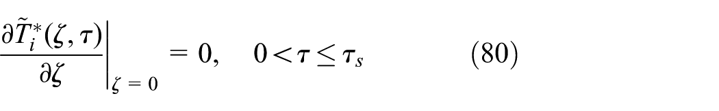
If $q_i^{*}(0)\ne 0$ , then from equation (78), it follows that the initial condition (67) is not satisfied. To correct the solution (77), we considered the following transient problem of the heat conduction with respect to dimensionless temperature ${\tilde{T}}_i^{*}$ , $i=1,2,...,10$

$$\frac{{\partial }^2{\tilde{T}}_i^{*}(\zeta ,\tau )}{\partial {\zeta }^2}=\frac{\partial {\tilde{T}}_i^{*}(\zeta ,\tau )}{\partial \tau },0<\zeta <1,0<\tau \le {\tau }_s$$

(79)

$${\frac{\partial {\tilde{T}}_i^{*}(\zeta ,\tau )}{\partial \zeta }|}_{\zeta =0}=0,0<\tau \le {\tau }_s$$

(80)

$${\frac{\partial {\tilde{T}}_i^{*}(\zeta ,\tau )}{\partial \zeta }|}_{\zeta =1}=0,0<\tau \le {\tau }_s$$

(81)

$${\tilde{T}}_i^{*}(\zeta ,0)=T_i^{*}(\zeta ,0),0\le \zeta \le 1$$

(82)

where the dimensionless temperature $T_i^{*}(\zeta ,0)$ has the form (78).

Figure 3.

Evolution of dimensionless density of the braking work $w_i^{*}(t)$ : (a) $i=1,2,...,6$ and (b) $i=7,8,910$ .

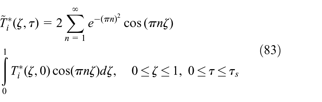
Solution of the boundary-value problem (79)–(82) has the following general form ²⁸

$$\begin{array}{l}{\tilde{T}}_i^{\ast }(\zeta ,\tau )=2{\displaystyle \sum _{n=1}^{\infty }{e}^{-{(\pi n)}^2}}\cos (\pi n\zeta )\\ {\displaystyle \underset{0}{\overset{1}{\int }}{T}_i^{\ast }(\zeta ,0)\cos }(\pi n\zeta )d\zeta ,0\le \zeta \le 1,0\le \tau \le {\tau }_s\end{array}$$

(83)

Substituting the function $T_i^{*}(\zeta ,0)$ (77) to the right side of equation (83) and integrating it, we obtained

$$\begin{array}{l}{\tilde{T}}_i^{\ast }(\zeta ,\tau )=2q_i^{\ast }(0){\displaystyle \sum _{n=1}^{\infty }\frac{e^{-{(\pi n)}^2\tau }}{{(\pi n)}^2}}\cos (\pi n\zeta ),\\ 0\le \zeta \le 1,0\le \tau \le {\tau }_s\end{array}$$

(84)

The difference between solutions (77) and (84) is

$$\begin{array}{c}{T}_i^{*}(\zeta ,\tau )=[\frac{1}{3}-\zeta (1-\frac{\zeta }{2})]q_i^{*}(\tau )+{\tau }_s{w}_i^{*}(\tau )\hfill \\ -2q_i^{*}(0)\sum _{n=1}^{\infty }\frac{e^{-{(\pi n)}^2\tau }}{{(\pi n)}^2}\cos (\pi n\zeta ),\hfill \\ 0\le \zeta \le 1,0\le \tau \le {\tau }_s,i=1,2,...,10\hfill \end{array}$$

(85)

is the wanted solution of the problem (64)–(67), presented in the Chichinadze’s monograph. ¹⁵ As it was shown above, this solution satisfies the boundary conditions (65) and (66), and taking into account the sum of series ²⁵

$$2\sum _{n=1}^{\infty }\frac{\cos (\pi n\zeta )}{{(\pi n)}^2}=\frac{1}{3}+\frac{1}{2}{\zeta }^2-\zeta =\frac{1}{3}+F(\zeta )$$

(86)

it also satisfies the initial condition (67). On the heated surface from the solution (85), we obtained

$$\begin{array}{l}{T}_i^{\ast }(0,\tau )=\frac{1}{3}{q}_i^{\ast }(\tau )+{\tau }_s{w}_i^{\ast }(\tau )-2q_i^{\ast }(0){\displaystyle \sum _{n=1}^{\infty }\frac{e^{-{(\pi n)}^2\tau }}{{(\pi n)}^2}},\\ 0\le \tau \le {\tau }_s,i=1,2,\dots ,10\end{array}$$

(87)

Solutions (85) and (87) provide the basis to calculate the average temperature of frictional surfaces in brake systems by means of solutions to the system equations of heat dynamics of friction and wear.^6,19 However, these solutions are approximate, because they have been obtained with a simplifying assumption (68). One of the aims of this article is to establish applicability limits of this solution by means of the numerical analysis presented below.

Numerical analysis

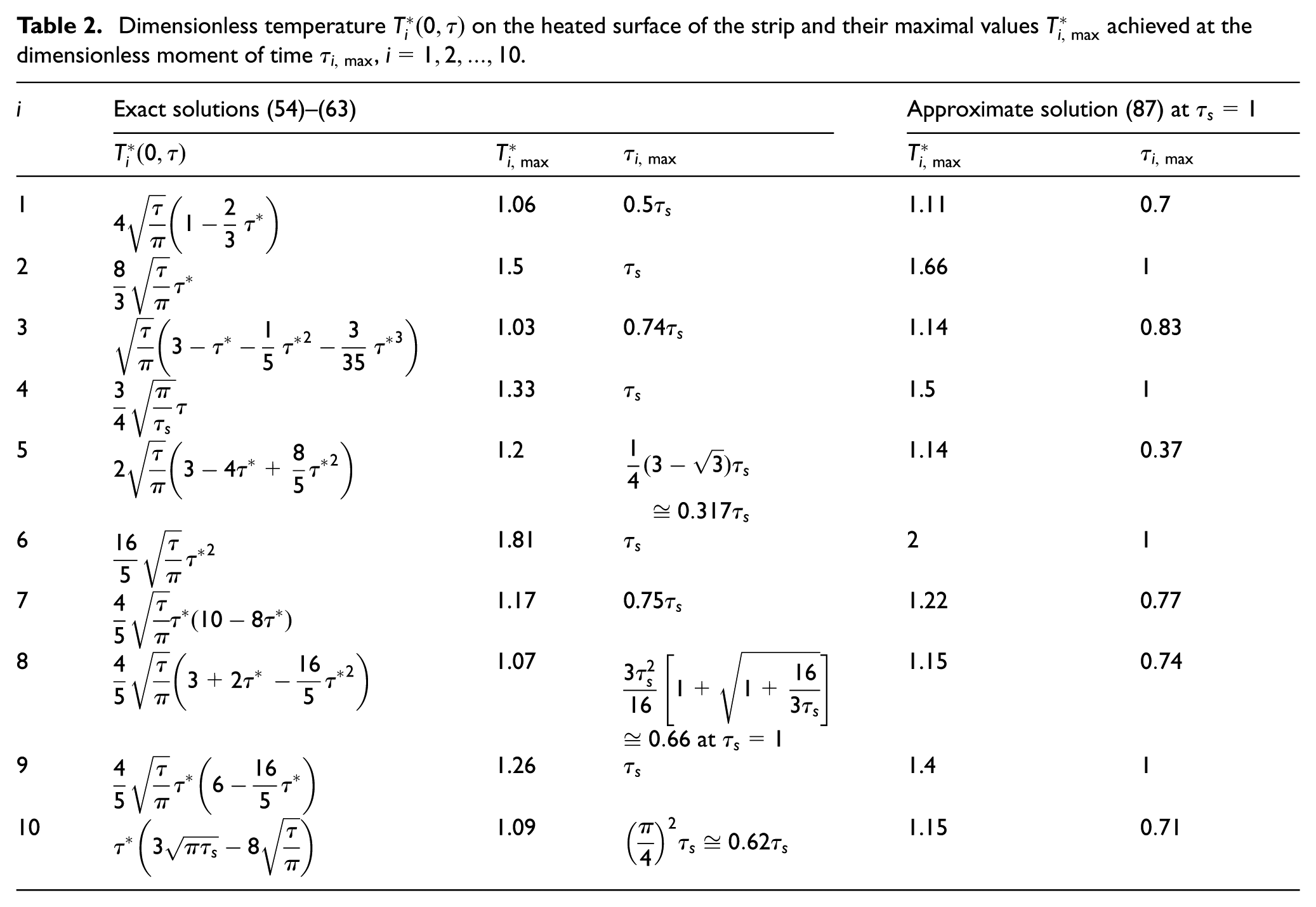
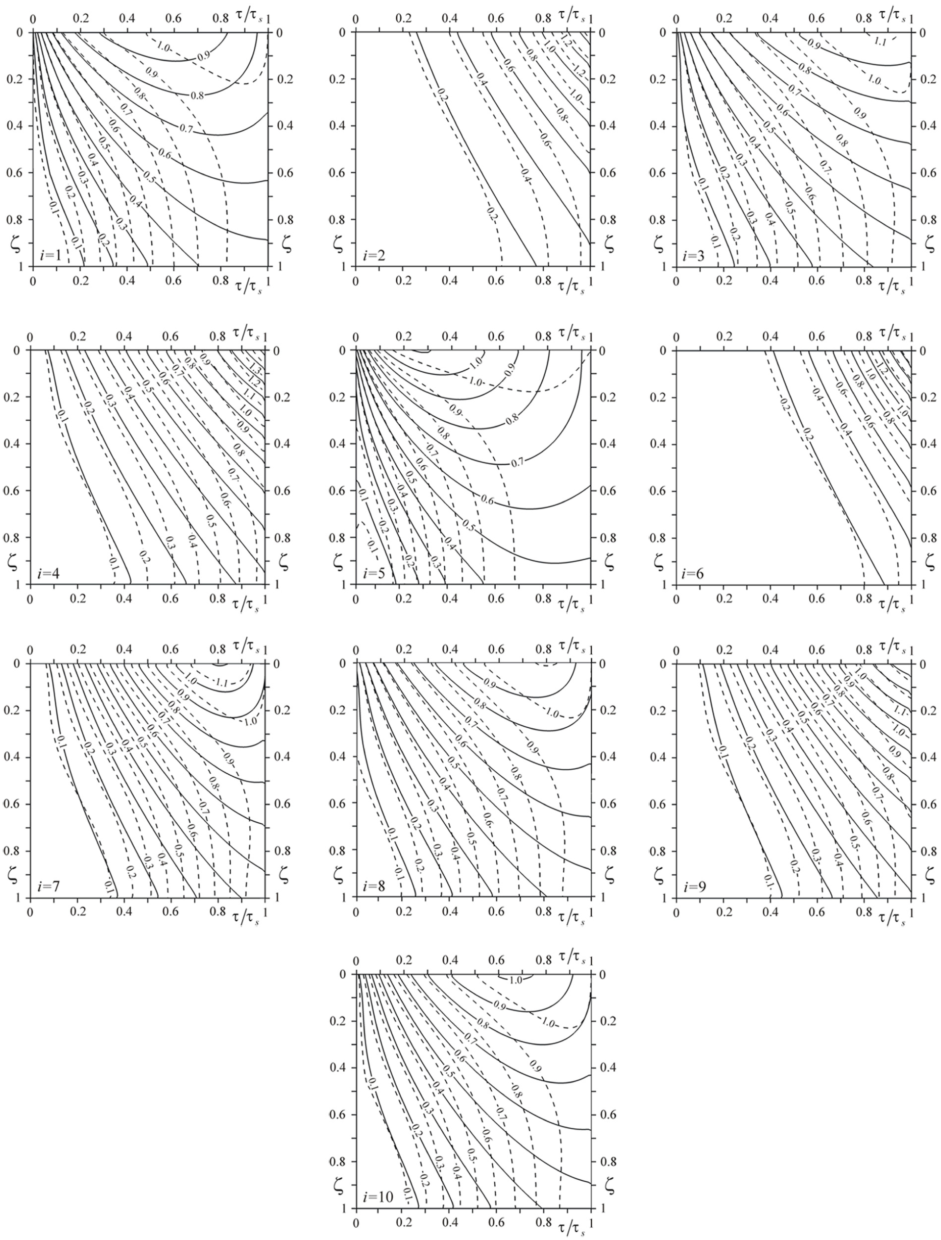
The dimensionless input parameters are the distance from the heated surface $\zeta$ and the Fourier numbers $\tau$ and ${\tau }_s$ (10). The formulas to calculate the dimensionless temperatures $T_i^{*}(0,\tau )$ , $i=1,2,...,10$ , on the heated surface $\zeta =0$ ( $Z=0$ ), obtained from exact solutions (50)–(59), are included in Table 2 and their graphs are shown by solid lines in Figure 4. The maximum values of the dimensionless temperatures $T_{i,max}^{*}$ and the moments of time $\tau ={\tau }_{i,max}$ , when they are achieved, calculated by means of exact (54)–(63) and approximate (87) solutions are contained in Table 2. The corresponding evolutions of dimensionless temperatures, obtained using the approximate solution (87), are shown by dashed lines in Figure 4. Comparing the evolutions of the temperatures obtained based on the exact solutions (solid lines) and the approximate solution (dashed lines), it can be seen that qualitatively temperature curves are close to each other. However, in quantitative terms, the approximate results overestimate the values of temperature up to 11% in comparison with results from the exact solutions.

Table 2.

Dimensionless temperature $T_i^{*}(0,\tau )$ on the heated surface of the strip and their maximal values $T_{i,max}^{*}$ achieved at the dimensionless moment of time ${\tau }_{i,max}$ , $i=1,2,...,10$ .

$i$	Exact solutions (54)–(63)			Approximate solution (87) at ${\tau }_s=1$
	$T_i^{*}(0,\tau )$	$T_{i,max}^{*}$	${\tau }_{i,max}$	$T_{i,max}^{*}$	${\tau }_{i,max}$
1	$4\sqrt{\frac{\tau }{\pi }}(1-\frac{2}{3}{\tau }^{*})$	1.06	$0.5{\tau }_s$	1.11	$0.7$
2	$\frac{8}{3}\sqrt{\frac{\tau }{\pi }}{\tau }^{*}$	1.5	${\tau }_s$	1.66	1
3	$\sqrt{\frac{\tau }{\pi }}(3-{\tau }^{*}-\frac{1}{5}{{\tau }^{*}}^2-\frac{3}{35}{{\tau }^{*}}^3)$	1.03	$0.74{\tau }_s$	1.14	$0.83$
4	$\frac{3}{4}\sqrt{\frac{\pi }{{\tau }_s}}\tau$	1.33	${\tau }_s$	1.5	$1$
5	$2\sqrt{\frac{\tau }{\pi }}(3-4{\tau }^{*}+\frac{8}{5}{{\tau }^{*}}^2)$	1.2	$\begin{array}{c}\frac{1}{4}(3-\sqrt{3}){\tau }_s\hfill \\ \cong 0.317{\tau }_s\hfill \end{array}$	1.14	$0.37$
6	$\frac{16}{5}\sqrt{\frac{\tau }{\pi }}{{\tau }^{*}}^2$	1.81	${\tau }_s$	2	1
7	$\frac{4}{5}\sqrt{\frac{\tau }{\pi }}{\tau }^{*}(10-8{\tau }^{*})$	1.17	0.75 ${\tau }_s$	1.22	0.77
8	$\frac{4}{5}\sqrt{\frac{\tau }{\pi }}(3+2{\tau }^{*}-\frac{16}{5}{{\tau }^{*}}^2)$	1.07	$\frac{3{\tau }_s^2}{16}[1+\sqrt{1+\frac{16}{3{\tau }_s}}]$ $\cong 0.66$ at ${\tau }_s=1$	1.15	$0.74$
9	$\frac{4}{5}\sqrt{\frac{\tau }{\pi }}{\tau }^{*}(6-\frac{16}{5}{\tau }^{*})$	1.26	${\tau }_s$	1.4	1
10	${\tau }^{*}(3\sqrt{\pi {\tau }_s}-8\sqrt{\frac{\tau }{\pi }})$	1.09	${\left(\frac{\pi }{4}\right)}^2{\tau }_s\cong 0.62{\tau }_s$	1.15	$0.71$

Figure 4.

Evolution of dimensionless temperature $T_i^{*}(0,\tau )$ on the heated surface: (a) $i=1,2,...,6$ and (b) $i=7,8,910$ . Solid lines represent exact solution, and dashed lines represent approximate solution.

The time profiles of the specific friction power, presented in Figure 2, can be classified into one of three groups. The first group includes curves with numbers $i=1,3,5$ , which reach maximum values at the initial time $\tau =0$ and monotonically decrease to zero at the stop time (Figure 2(a)). The graph of the function $q_1^{*}(t)$ is linear, and the corresponding dimensionless temperature reaches its maximum $T_{1,max}^{*}=1.06$ in the middle of the braking process at $\tau =0.5{\tau }_s$ (Figure 3(a); Table 2), which is specific for braking with constant retardation. ¹ The graphs of the functions $q_i^{*}(t)$ , $i=3,5$ , are parabolas (concave at $i=3$ and convex at $i=5$ ), which decrease from the maximum value $q_{i,max}^{*}=1.5,3$ , $i=3,5$ , at $t=0$ to 0 at the stop moment $t=t_s$ (Figure 2(a)). The corresponding values of maximum temperature $T_{i,max}^{*}=1.03,1.2$ at $i=3,5$ are achieved at moments of time ${\tau }_{i,max}=0.74{\tau }_s,0.32{\tau }_s$ , $i=3,5$ (Figure 4(a), Table 2).

The second group comprises the specific power of friction $q_i^{*}(t)$ , $i=2,4,6$ (Figure 2(a)). These functions monotonically increase from zero at the initial time to the maximum values $q_{i,max}^{*}=2,1.5,3$ , $i=2,4,6$ , at the stop time (Table 1). In the similar way, corresponding dimensionless temperatures $T_i^{*}(0,\tau ),i=2,4,6$ (Figure 4(a)) change with time. The maximum values of these temperatures at the moment of stop are $T_{i,max}^{*}=1.5,1.33,1.81$ for $i=2,4,6$ , respectively (Table 2).

The third group includes the temporal profiles of specific friction power $q_i^{*}(t)$ , $i=7,8,910$ , which has a local maximum within a time braking interval $0\le \tau \le {\tau }_s$ (Figure 2(b)). The values of local maximum of the functions $q_i^{*}(t)$ , $i=7,8,910$ , are achieved at the time moments $t_{i,max}=0.5t_s,0.25t_s,0.75t_s,0.25t_s$ , respectively (Table 1). The corresponding dimensionless temperatures $T_i^{*}(0,\tau )$ also rise with the beginning of braking until they reach the maximum values $T_{i,max}^{*}=1.17,1.07,1.26,1.09$ , $i=7,8,910$ (Table 2). Then, in the cases $i=7,8,10$ , cooling of the friction surface follows, but when $i=9$ , the temperature increases till the moment of stop (Figure 4(b)).

Isolines of the dimensionless temperature $T_i^{*}(\zeta ,\tau )$ , $i=1,2,...,10$ , calculated on the basis of exact solutions (54)–(63) (the solid curves) and approximate solution (85) (the dashed curves), are presented in Figure 5. On the friction surface, exact and approximate temperature values are comparatively close to each other. However, differences between these results significantly increase with the increasing distance from the heated surface (Figure 5). The lower the dimensionless time ${\tau }_{i,max}$ to reach the maximum temperature, the more intensive a cooling process and the more non-linear the shape of isotherms. Whereas a monotonic increase in temperature during the whole braking process in cases $i=2,4,6,9$ in Figure 4 corresponds to a linear lowering of the temperature at a distance from the heated surface (Figure 5). In these cases, for which ${\tau }_{i,max}={\tau }_s$ , we can observe (Figure 5) the smallest difference between solid and dashed lines. The longer the time ${\tau }_{i,max}$ , the more closer the isolines obtained based on exact and approximate solutions, considering range of depth to be $0\le \zeta \le 1$ .

Figure 5.

Isolines of dimensionless temperature $T_i^{*}(\zeta ,\tau )$ : (a) $i=1,2,...,6$ and (b) $i=7,8,910$ . Solid lines represent exact solution, and dashed lines represent approximate solution.

Distributions of isotherms at a depth from the heated surface reflect the evolution of the temperature on that surface (Figure 5). The greatest concentration of isolines occurs inside a semi-space, near the places on the heated surface where the maximum temperature is reached. The higher the maximum temperature on the heated surface, the faster the whole analyzed spatial region $0\le \zeta \le 1$ gets overheated.

Conclusion

In this article, a comparative analysis of the influence of specific friction power on the temperature of friction element in braking system has been presented. A total of 10 different functions have been selected that describe the time profiles of the specific power of friction from the monograph. ¹⁵ Such processes of braking have been considered, in which an identical total braking work was made at the same braking time. For one of the elements of the brake system, a one-dimensional boundary-value problem of heat conductivity with frictional heating at single braking has been formulated. The exact solution of this problem for all the above-mentioned 10 temporal profiles of the specific friction power has been obtained. By using these solutions, the numerical analysis of the spatial-time temperature distributions has been made. Evolutions of the temperature on the heated surface obtained from exact solution have been compared to the corresponding temperatures calculated using an approximate solution from monograph. ¹⁵ It has been established that the approximate solution overstate the value of maximum temperature to not more than 11% in comparison with the exact solution. By increasing the distance from the heated surface, the differences between temperature values calculated based on exact and approximate solutions rapidly increase. It follows that approximate Chichinadze’s solution ¹⁵ gives acceptable results during calculating the temperature of the contact surface (e.g. average temperature of this surface). However, using this solution during calculating a volumetric temperature of the friction element can lead to considerable errors.

It has been established that the shape of the temporal profile of the specific friction power and time of appearance of the maximum value have a significant influence on both the evolution of the surface temperature and the temperature distribution inside the friction element. There is a direct relation between the maximum value of the specific power of friction and temperature. The greater the time to reach the highest value of specific power of friction, the greater the time for temperature to reach its maximum value.