Sage Journals: Discover world-class research

Abstract

For pick-and-place processes to become widely implemented in industry a consistent and acceptable product quality needs to be achieved. In the state of the art it is assumed that reinforcements will be in perfect condition at the start of forming or draping. In reality the handling process can already result in undesired deformations. The current work will look at fiber angle deviations that occur during this process due to in-plane shear. It is shown that bounds can be set for these fiber angle deviations based on experimental work. Periodic representative volume element homogenization is used to obtain homogenized material properties for a bi-axial non-crimp fabric with a specific construction. With these material properties the in-plane shear strain, and thus the fiber angle deviations, can be predicted. The presented methodology and results obtained using it can be a basis in the design process for automated handling of reinforcements and for in-situ quality control of the pick-and-place process.

Keywords

composite fabrics performance composites technical nonwoven fabrics high performance fabrics structure properties

Introduction

Implementation of the pick-and-place process in industry requires a consistent and acceptable product quality. Without quality criteria it is not possible to evaluate the quality of the process and final product. In the state of the art on handling of (non-crimp) fabrics using pick-and-place operations quality criteria are often overlooked. The quality criterion that is most often reported in literature is a placement accuracy/repeatability. Martinsson¹ uses an array sensor to measure the position of the edges of a placed prepreg relative to predefined points. Kuehnel, Schuester, Buchheim, Gerngross and Kupke² use a computer vision approach to detect position and orientation of cuts before picking them up and placing them. Krogh et al.³ discuss the off-set between prescribed and actual boundaries for their numerical simulations of draping of woven prepregs on double curved molds. Additionally, they also report the ply-mold separation for different draping strategies. The work by Gerngross and Nieberl⁴ stands out because they set tolerances for both the fiber angles (±5°) and the boundary curve positions (+5/-7.5 mm). Their preforming results are evaluated by comparing them to a laser projection.

One of the most important quality criterions and design parameters for fiber reinforced materials is the orientation of the fibers. Fibers loaded in the axial direction will have a positive impact on the strength and stiffness of a product. A misalignment between the fiber direction and the loading direction will greatly reduce these mechanical properties. This is e.g. illustrated by Mouritz⁵ for a UD composite loaded at different angles. The orientation of the fiber angles should therefore be taken into account when the pick-and-place process is studied.

Fiber angles are directly influenced by in-plane shear. In-plane shear is the main deformation mode during forming of reinforcements⁶ and will also be the main deformation mode during handling. In-plane shear angles of the final product are a common result presented in studies focusing on forming and draping. Recent work includes the draping simulations of Guzman-Maldonado, Bel, Bloom, Fideu and Boisse⁶ for non-orthogonal biaxial NCFs. Krieger, Gries and Stapleton⁷ present optically measured local shear angles for non-crimp fabrics with different stitch types and orientations. Wang, Wang, Hamila and Boisse⁸ produce both experimental and simulated results for the in-plane shear angle for hemispherical stamping of 3D woven composite reinforcements.

Handling a reinforcement will subject it to forces due to e.g. gravity and accelerations. These forces can result in deformations and therefore in deviations of the fiber angles. Deformations during handling using pick-and-place operations are for example presented by Krogh, Sherwood and Jakobsen⁹ in the context of generating feasible gripper trajectories for the draping of prepregs. Lin, Clifford, Taylor and Long¹⁰ and Do, John and Herszberg¹¹ are examples of studies interested in predicting the deformations of reinforcements during handling in real time.

One factor that will have a large influence on the behavior of a reinforcement that is handled is the positioning of pick-up points. Ragunathan and Karunamoorthy¹² and Lankalapalli and Eischen¹³ studied the optimal positioning of pick-up points based on minimization of strain energy. Ballier¹⁴ based the positioning of pick-up points on deflections. These parameters do however not give a clear indication of the quality of the reinforcement. With fiber angles being such an important parameter for the quality of a composite product fiber angle deviations should be taken into account when designing the pick-and-place process. Tolerances need to be set for the in-plane shear and resulting fiber angle deviations. Pick-up points need to be positioned in a way that ensures that deviations remain within the previously established boundaries.

Until now, no clear bounds have been established for fiber angle deviations during handling of different non-crimp fabrics. Therefore, the aim of this paper is to provide a framework for the determination of acceptable criteria for in-plane shear induced fiber angle deviations in bi-axial non-crimp fabrics. For the current work the filaments within a tow are assumed to be aligned to such an extent that tow angles correspond to filament angles, factors such as in-plane waviness as a result of manufacturing are not considered. First, experimental picture frame tests are used to set a tolerance for the fiber angle deviations/in-plane shear strain. The simulated shear response can be used as an indication of fiber angle deviations. Next, representative volume elements [RVEs] and periodic RVE homogenization are used to determine the material properties for an NCF with a specific stitching pattern and dimension. These material properties can then be used in future simulations. The results from these simulations can be analyzed using the tolerances determined as described in the current work. The next section discusses the results from the current work. Finally, the conclusions are presented.

Fiber angle deviations and in-plane shear in an NCF

For the current work an E-glass based Biaxial ± 45^o NCF with a chain stitch pattern is used. A chain-stitch type NCF has been chosen since a chain stitch gives a high form stability, making the fabric appropriate for automated handling.⁷ Figure 1 illustrates the stitch pattern of the NCF. Table 1 presents the details for the NCF selected for the present work.

Figure 1.

Stitch pattern of NCF. The vertical red line indicate he direction of the stitches, the diagonal black lines indicate the direction of the fibers of the top layer.

Table 1.

Specifications of selected fabric provided by manufacturer.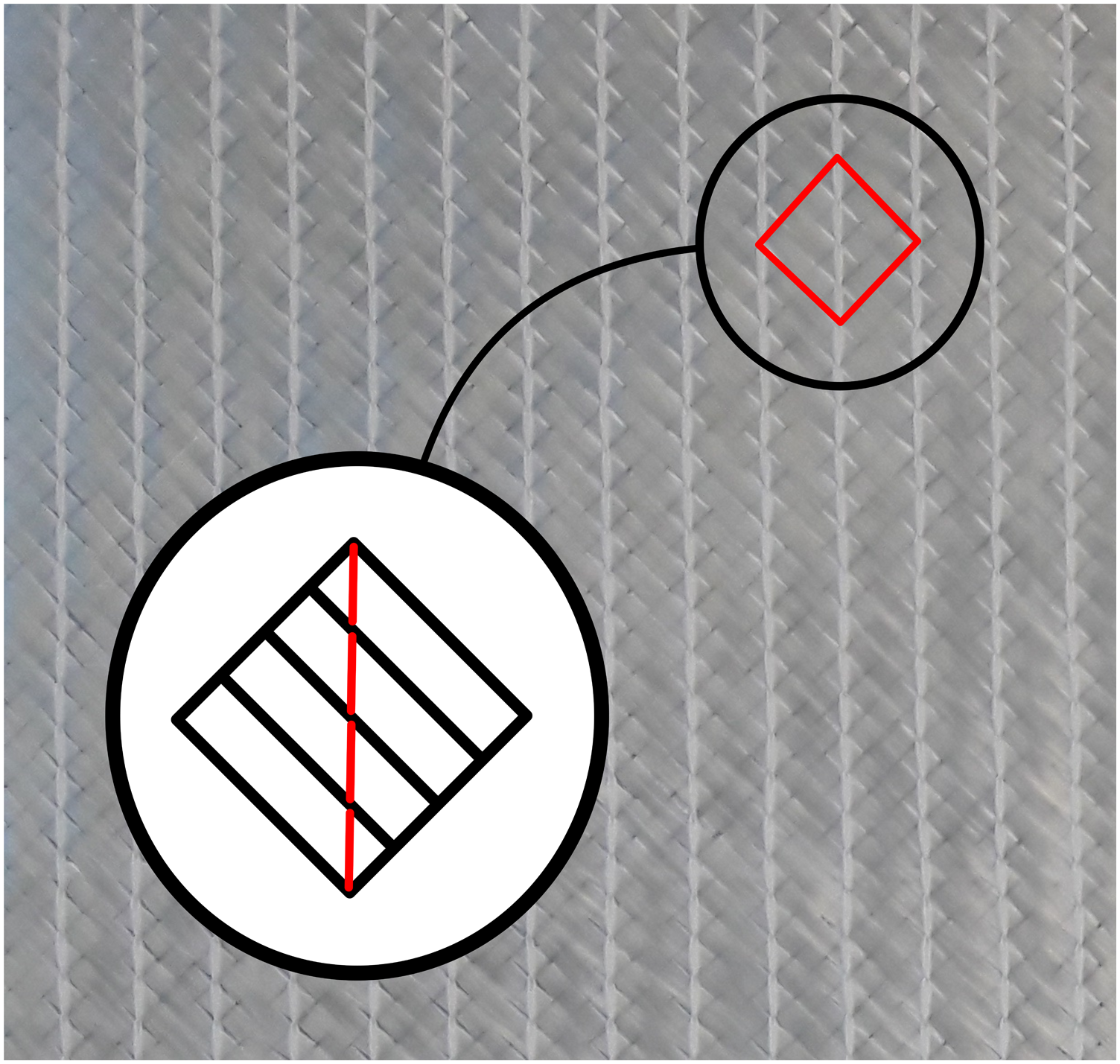

Fabric type	Biaxial ± 45^o NCF
Weight	430 g/m²
Fibres	100% E-glass (300 tex)
Stitch	Chain stitch
Finishing	Silane treated

There is no standard for the shear testing of biaxial fabrics like the NCF used in this work. A test that is widely used to characterize the in-plane shear behavior of non-crimp fabrics is the picture frame test. Recent work using this test includes e.g. Guzman-Maldonado et al.⁶ and Habboush, Sanbhal, Shao, Jiang and Chen.¹⁵ The current work will also use the picture frame test.

In a picture frame test the fabric is constrained at the edges and subjected to pure shear. Figure 2 shows a schematic of the aluminum frame used to clamp the fabric on four edges and both specimens with stitches loaded in tension and with stitches loaded in compression. The red stripes in the figures indicate the direction of the stitches while the blue lines indicate the direction of the fibers. The fabrics’ stabilizing yarns in the 0/90 direction are removed prior to testing.

Figure 2.

Illustration of the frame design and both a tension and compression specimen with the direction of the stitches indicated in red stripes and the direction of the fibers indicated in blue lines.

Figure 3 shows the picture frame with a specimen clamped during testing. Several tows are highlighted using black marker to track the behavior of the tows during testing. Pictures are taken so the tow angles can be compared to the frame angles in post-processing.

Figure 3.

Picture frame with clamped fabric during testing.

To ensure that the start of the test coincides with the start of shearing, the distance between opposite holes in the specimens is 1 mm smaller than the distance between opposite holes in the frame. Double sided tape is applied to fix the specimens to the frame, thereby eliminating the possibility of slipping. During the test the load-displacement curve is recorded using a 10 N load cell. A camera set-up is used to monitor the fabric. Specimens are tested at a speed of 10 mm/min. Machine speed is based on the work by Lomov¹⁶ who found no systemic variation of the shear resistance of biaxial non-crimp fabrics when using machine speeds from 10 to 1000 mm/min. Curves were observed to change within the experimental scatter range.

Load-displacement data is automatically recorded by the tensile testing machine. The load-displacement curve due to shear of the specimen is obtained by subtracting the load-displacement curves for each test by the relevant load-displacement curve for the empty frame. Each test is repeated three times. The initial cycle will be a conditioning cycle during which the specimen settles, ensuring a uniform response of the fabric.¹⁶ Unless noted otherwise the values presented in this work are the average of the second and third cycle.

The current work studies fiber angle deviations due to in-plane shear in the context of material handling in the composite manufacturing process. This means that the region of interest is different than other work carrying out picture frame tests. Typically, specimens will be tested up to the locking angle. Recent examples include the work by Fial, Carosella, Ring and Middendorf,¹⁷ Lux, Fial, Schmidt, Carosella, Middendorf and Fox¹⁸ and Balakrishnan, Yellur, Roesch, Ulke-Winter and Seidlitz.¹⁹ For the current work the interest lays in the unintended deviations that may occur during to the handling process. With this in mind specimens are initially tested over a range of displacements from 1 to 10 mm or frame angles from 0.47 to 4.68°. Based on these results the region of interest is further narrowed down to displacements of 1–5 mm (0.47–2.34°) and additional specimens are tested. Specimens are loaded up to a predefined displacement/angle. When this displacement has been reached the machine returns to its starting position. Once the starting position has been reached the next displacement/angle is applied.

Figure 4 shows load-displacement graphs for a compression specimen (a) and a tension specimen (b) loaded from 1 to 10 mm/0.47–4.68°. Figure 5 presents three compression and three tension specimens loaded from 1 to 5 mm/0.47–2.34°. Applied displacements have been converted to applied angles using basic trigonometry. For the current work the choice has been made to present results individually, as opposed to presenting a mean with standard deviations. The interest of the current work lays in setting tolerances for the fiber angle deviations based on the behavior of the fabric. Looking at individual specimens ensures that no behavior gets lost.

Figure 4.

Load-displacement graphs for compression and tension specimens for displacements of 1–10 mm: (a) Compression, (b) Tension.

Figure 5.

Load displacement graphs for compression and tension specimens for displacement of 1–5 mm. (a) Compression specimen 1, (b) Tension specimen 1, (c) Compression specimen 2, (d) Tension specimen 2, (e) Compression specimen 3, (f) Tension specimen 3.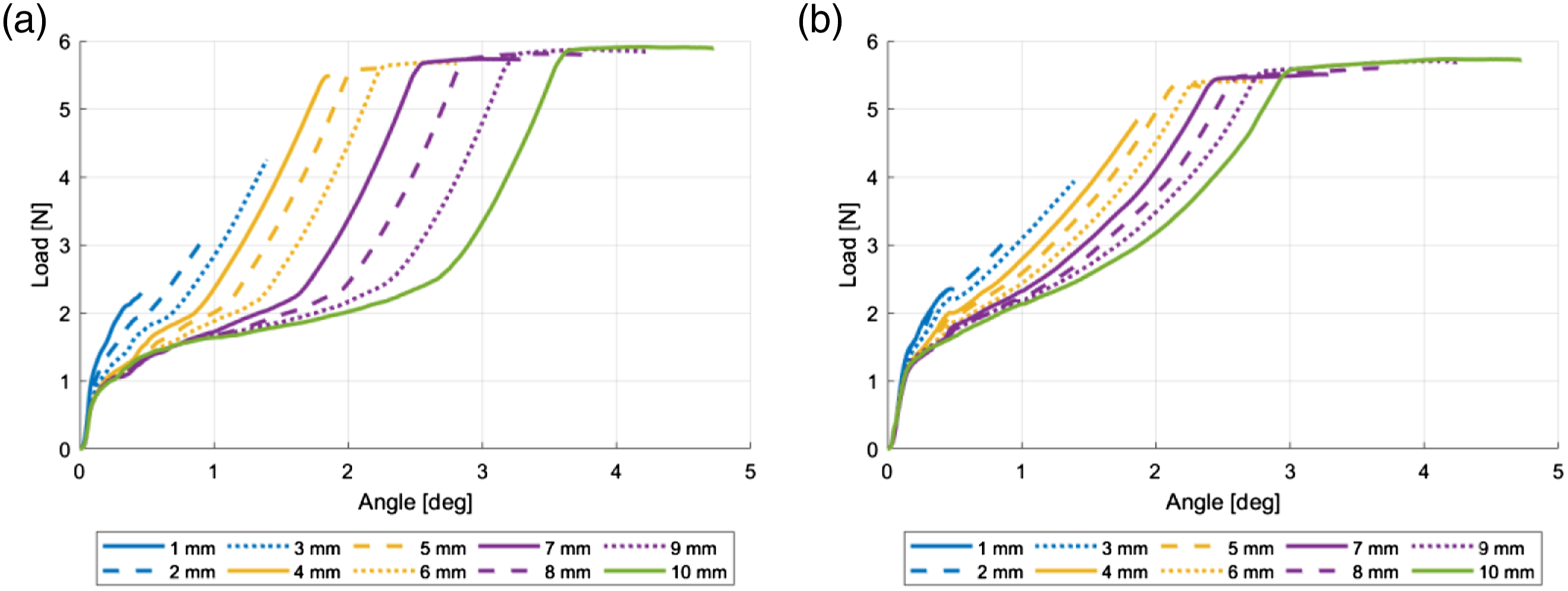

The initial steep region, observed for the curves in Figure 4 and Figure 5, is attributed to frame effects. Most frame effects have been removed from the data through subtraction of load-displacement data for empty frames. It is suggested that the presence of the preloaded fabric in the frame causes the frame to behave slightly different than in the empty cases. This results in the data still showing some behaviors that are not caused by shearing of the fabric.

The sudden change in trajectory at the end of the load-displacement graphs marks the point where the mechanical safety stop of the load cell is engaged. The 10 N load cell has been used despite this phenomena to ensure the highest accuracy in recording the load-displacement behavior in the region of interest: low displacements corresponding to low deviations in fiber angles. When a 10 kN load cell is used the load-displacement graphs will continue on their current trajectory until the set displacement is reached.

Setting limits for in-plane shear and fiber angle deviations based on the picture frame tests

When setting bounds for the fiber angle deviations they should be set such that no irreversible change has occurred yet. Figure 6 illustrates how the behavior of the fabric is influenced by previous shearing. The graphs present the load-displacement diagrams for applied displacements of 1, 3 and 5 mm, which corresponds to applied angles of 0.47, 1.40 and 2.34°. The ”5 -” notation indicates that these test cycles occurred after the frame had already been sheared up to 5 mm and returned back to the base position. The results show that the trajectory of these load-displacement graphs closely follows that of the 5 mm case. It requires significantly less force to shear the fabric to 3 mm once it has previously been sheared to 5 mm than if the fabric is new and unsheared. This shows that even at low displacements irreversible changes have already occurred in the fabric.

Figure 6.

Load-displacement graphs for a compression (a) and tension (b) specimen that is loaded at a series of lower and higher displacements.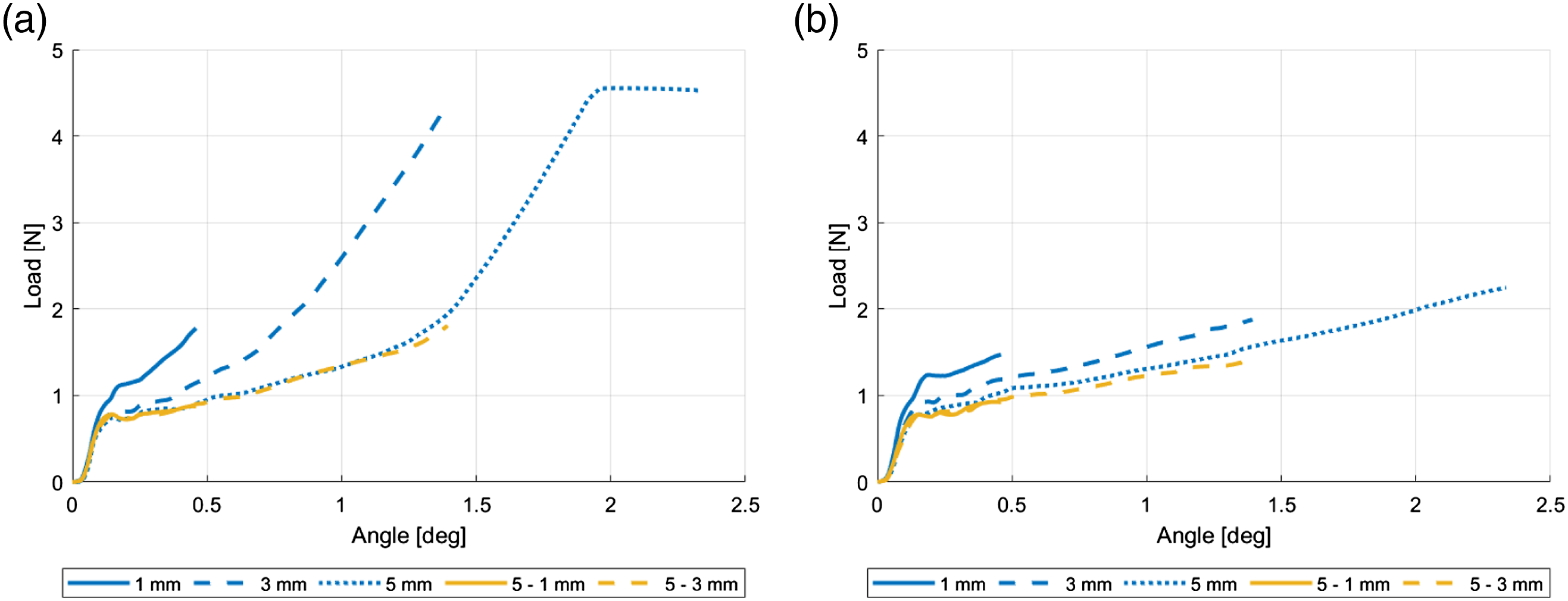

This behavior can also be seen in the results presented in Figure 4 and Figure 5. The slope for the final region of the curves for compression specimens remains consistent across the applied displacements of 1–10 mm. For the first region there is however a clear drop in resistance as the applied displacement increases. This is attributed to the behavior shown in Figure 6. Based on these observations the tolerance for the current work is set to displacements of 3 mm/angles of 1.4°.

Figure 7 shows the tows and frame arms that are used to compare the frame angles and the angles of the reinforcement during testing. For the reinforcement the angles are recorded at six different locations while for the frame the angles of all four frame arms are recorded. The angles of these six tows are individually compared to the average angle of the corresponding two parallel frame arms. The angles are measured using Inkscape.

Figure 7.

Highlighted tows and frame arms to indicate which angles are used in the comparison between frame angles and angles of the reinforcement during testing.

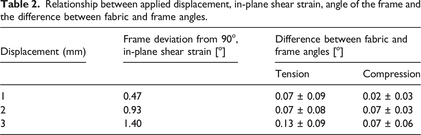
Basic trigonometry is used to convert the displacements of the picture frame to angles of the picture frame. This can then be used to calculate the in-plane shear strain. Table 2 shows these results and the average observed difference between the angles of the fabric specimens and the frame. From this it is concluded that the angles of the frame can also be used for the fiber angle deviations.

Table 2.

Relationship between applied displacement, in-plane shear strain, angle of the frame and the difference between fabric and frame angles.

Displacement (mm)	Frame deviation from 90^o, in-plane shear strain [ ^o ]	Difference between fabric and frame angles [ ^o ]
		Tension	Compression
1	0.47	0.07 ± 0.09	0.02 ± 0.03
2	0.93	0.07 ± 0.08	0.07 ± 0.03
3	1.40	0.13 ± 0.09	0.07 ± 0.06

Periodic RVE homogenization

A practical approach to evaluating reinforcement shear during handling is the use of existing Finite Element Analysis [FEA] software. For the current work the NCF is modeled on a mesoscale using a representative volume element [RVE]. An RVE can be defined as the smallest material volume element for which the macroscopic constitutive representation is a sufficiently accurate model to represent mean constitutive response.²⁰ Periodic RVE homogenization is used to get homogenized elastic properties for the NCF. These elastic properties can then be used in macro scale models of the NCF. In periodic RVE homogenization effective elastic properties are computed through imposition of uniform strains on the RVE.²¹

Setting up the RVE

Homogenized material properties are obtained through periodic RVE homogenization. The periodic RVE homogenization implementation is based on the work by Omairey et al.²¹ In that work the authors present EasyPBC, an ABAQUS/CAE plugin that calculates the homogenized effective elastic properties of RVEs created by the user. However, their algorithm is not compatible with RVEs that require multiple components for a correct representation, as is the case with non-crimp fabrics. For the current work the algorithm of EasyPBC 1.4 has been modified to work with an RVE that is build up using multiple tows and stitches.

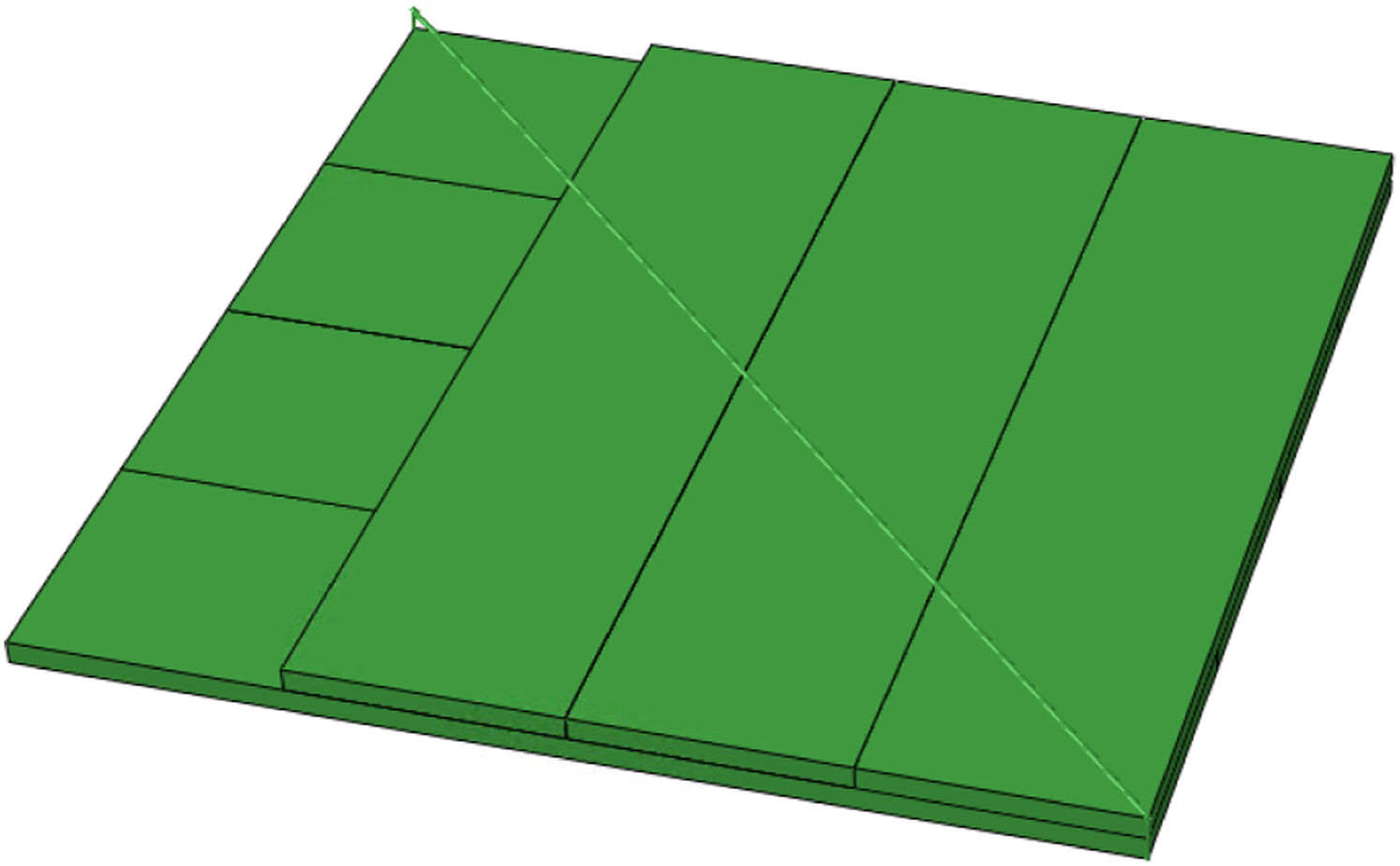
The algorithm written for the current work writes the input file for Abaqus based on input dimensions. Stitch patterns are defined by giving the trajectory of the simplified stitch using coordinates and specifying whether the stitch is to be attached to the top or bottom of the RVE. The stitch pattern of the NCF used in this work requires that at least four tows on the top and four tows on the bottom are used. The stitch pattern has previously been illustrated in Figure 1. Figure 8 shows the stitch pattern used in the RVE in red. Figure 9 shows the RVE with a top tow removed to show the bottom tows. In this figure the top part of stitches can still be seen as a diagonal line.

Figure 8.

The stitches in RVE are indicated in red.

Figure 9.

RVE with a top tow removed to show the bottom tows.

Within the model, tows are free to move relative to each other within the constraints of the boundary conditions used for periodic RVE homogenization as described by Omairey et al.²¹ The stitches are connected to the tows at each corner.

The stitching in a non-crimp fabric [NCF] has a large influence on the shearing behavior through the stitching pattern and their placement relative to the shearing motion.^22,23,7 Therefore, care has to be taken that the stitching pattern in the RVE is a good representation of the real life pattern. Figure 10 shows a reproduction of the chain stitch. On the front of the stitch there is a loop, on the back of the stitch there is a single thread. The stitching pattern highlighted in Figure 8 accounts for this by having twice the surface area for the top truss of each individual stitch.

Figure 10.

Reproduction of chain stitch; (a) Front, (b) Back.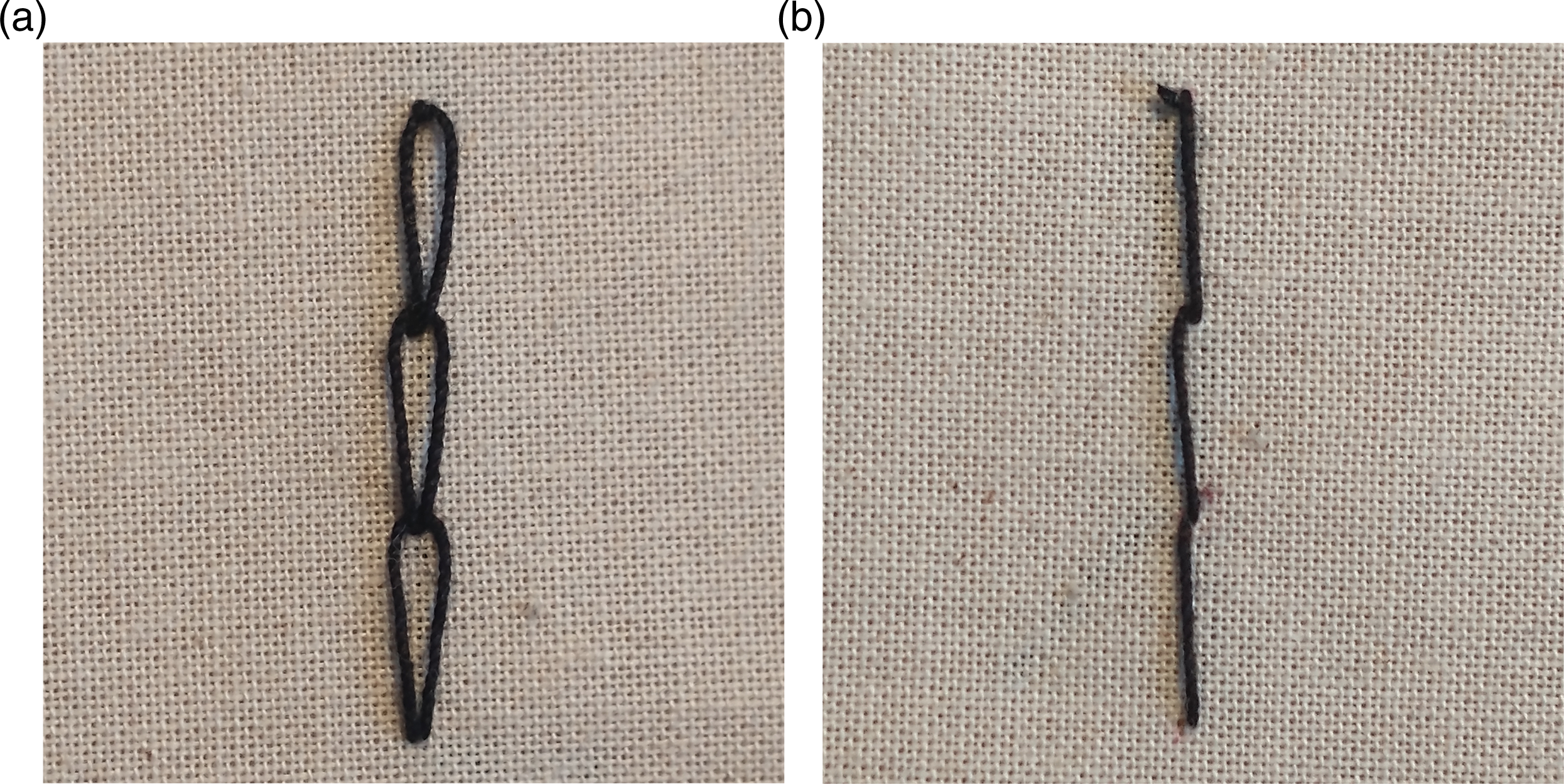

The dimensions required for modeling of the RVE that are not readily available are obtained using a micrometer and caliper. For the stitches a Young’s Modulus of 2.8 GPa is used for the PES material.^24,14

Figure 11 shows the meshed RVE model with dimensions. Here, ‘a’ is the width of a tow which is 1.89 mm. ‘b’ is four times the width of a tow and is 7.56 mm. ‘h’ is twice the thickness of a tow and is 0.168 x 2 = 0.336 mm. The surface area of a truss is 0.00159 mm² and double for the top truss. Within the RVE the tows are meshed using C3D8R elements with a size of 1/3 of the tow height, which is 0.168/3 = 0.056 mm. For the stitches T3D2 elements are used, with element size being equal to the dimensions of the individual stitch parts.

Figure 11.

Meshed RVE model with dimensions.

Obtaining tow properties for RVE input

A flexural rigidity test based on ASTM D1368 is used to approximate the longitudinal stiffness of the tow that ensures correct bending behavior. Similar approaches have previously been used by Creech and Pickett,²⁵ Pabst, Krzywinski, Schenk and Thomaszewski²⁶ and Döbrich, Gereke, Diestel, Krzywinski and Cherif²⁷ to calibrate mechanical properties to ensure correct behavior of fabric models.

Figure 12 shows how a tow is slid over a block with a 41.5^◦ slope until the tow hits the slope. L_residual and L_slope are recorded with an accuracy of 1 mm based on a ruler taped to the surface. These values are used to calculate L_over and δ. Next, linear elastic beam theory is used to obtain an initial approximation for the effective E₁₁.

Figure 12.

Flexural rigidity test block and tow with dimensions recorded during testing.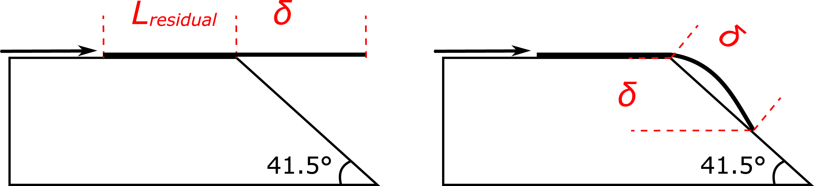

Eleven specimens have been tested using the procedure described above. From these experiments the resulting L_over is 133 ± 6 mm. The recorded L_slope is 129 ± 6 mm. The measured deflection, δ is 85 ± 4 mm. This value is used to calibrate the Young’s moduli to be used in the rest of the work.

E₁₁ is further calibrated using Abaqus/CAE 2017 through a non-linear shell model of the beam deflection test. In the model one end of the tow is fixed in all rotational and translational degrees of freedom and a gravitational load of 9.81 m/s² is applied. The model is meshed using S4R elements with a mesh size equal to the tow width of 1.89 mm. Figure 13 shows a schematic of the model used for the overhang test simulations. The width ‘a’ and thickness ‘h’ of the model are equal to tow dimensions and respectively 1.89 mm and 0.168 mm. Length ‘b’ is the mean overhang length recording during the experiments and is 133 mm.

Figure 13.

Schematic of overhang test simulation.

The longitudinal stiffness is varied until the tow deflection matches the experimental work. Based on the observations that the deflection is virtually independent on the magnitude of E₂₂ and E₃₃ these stiffnesses are set at E₁₁/10.

Figure 14 shows the simulation results compared to the average measurements for the tow end. For the simulation with elastic properties based on linear elastic beam theory E₁₁ = 2.48 GPa and E₂₂, E₃₃ = 248 MPa. The calibrated Young’s moduli are E₁₁ = 1.57 GPa and E₂₂, E₃₃ = 157 MPa. This is considerably lower than a typical Young’s modulus for E-glass of 72 GPa.

Figure 14.

Simulation results compared to experimental measurements of the tow end deflection.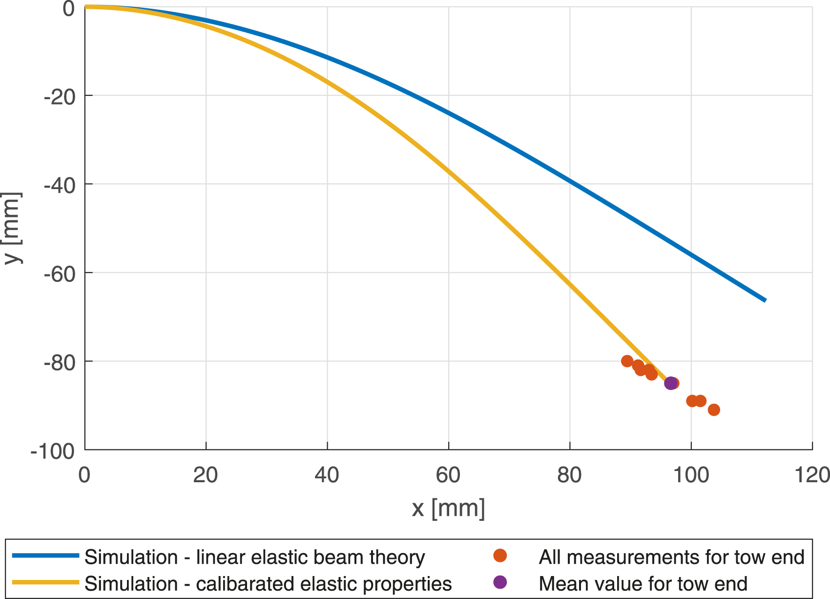

The explanation for this difference is twofold. Firstly, this typical Young’s modulus is an axial modulus. This modulus will only be identical to a Young’s modulus calibrated for bending if the material behaves perfectly linear. The second part of the explanation lays in the construction of a tow. A tow is not solid E-glass: it’s made up of a bundle of E-glass filaments. When loaded in tension the bundle of filaments might act very similarly to solid E-glass with the same dimensions. However, for bending the internal mechanisms between the two cases will be different. For solid E-glass the bending will purely come from bending of the material. The filaments in the tows will have a low resistance to bending due to their small dimensions. Friction between the filaments causes them to connect and show a larger resistance to deformation. The combination between bending of individual filaments and the friction results in an effective bending stiffness for a tow.

For the tows a constant volume assumption is used which gives Poisson’s ratio’s μ₁₂ = μ₂₃ = μ₁₃ = 0.5. Creech²⁵ found it suitable to take all shear moduli to be equal.

The shear moduli of the tows are calibrated by looking at the homogenized in-plane shear modulus of the NCF. In real life an NCF will not have any resistance to in-plane shear without the stitches, the response of the RVE should reflect this. The tow shear moduli are varied until the RVE gives the desired response: matching the real life behavior as close as possible while ensuring computational time is kept reasonable. This results in shear moduli for the tows of 0.65 MPa.

Table 3 Summarizes the final tow input values that are used.

Table 3.

Tow elastic properties used in RVE.

E₁₁ ^(MPa)	E₂₂ ^(MPa)	E₃₃ ^(MPa)	μ₁₂ ^[-]	μ₁₃ ^[-]	μ₂₃ ^[-]	G₁₂ ^(MPa)	G₁₃ ^(MPa)	G₂₃ ^(MPa)
1570	157	157	0.5	0.5	0.5	0.65	0.65	0.65

Determination of homogenized material properties using the RVE

Table 4 shows the homogenized properties calculated using the RVE based on tow and stitch properties as determined previously. This section will go over the elastic properties and where required update these initial results.

Table 4.

Homogenized elastic properties as determined by the RVE based on previously determined tow and stitch properties.

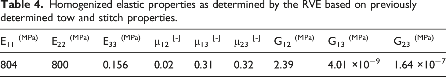
E₁₁ ^(MPa)	E₂₂ ^(MPa)	E₃₃ ^(MPa)	μ₁₂ ^[-]	μ₁₃ ^[-]	μ₂₃ ^[-]	G₁₂ ^(MPa)	G₁₃ ^(MPa)	G₂₃ ^(MPa)
804	800	0.156	0.02	0.31	0.32	2.39	4.01 ×10⁻⁹	1.64 ×10⁻⁷

The RVE determines elastic properties by applying displacements in the 1, 2 and 3 direction. It is unable to determine properties calibrated for bending. Therefore, the E₁₁ and E₂₂ presented in Table 4 are an overestimate. E₁₁ and E₂₂ calibrated for bending can however easily be estimated by looking at EI instead of just E. The method is also shown for the standard axial stiffness to demonstrate the validity of properties determined using these steps.

The stiffness E₁₁ for the tows has been determined to be 1570 MPa. With the definitions chosen for the RVE the tows lay in the 1 and 2 direction. It is assumed that tows perpendicular to the loading direction will not contribute. This means that only half the height of the fabric will be available in both the A in EA and the I in EI.

If the full height would contribute, the E₁₁ of the fabric would be the same as the E₁₁ of a tow. With only half the height contributing EA can be written as $E \cdot \frac{1}{2} h \cdot b$ or $\frac{1}{2} E A$ . Since in the homogenized part, the full area is used, the E-modulus has to be halved, leading to E₁₁ = 785 MPa, which is close to the 800 MPa found by the RVE.

The same can be done for EI. Writing EI out results in $E \cdot b \cdot {(\frac{1}{2} h)}^{3} / 12$ or $\frac{1}{8} E I$ . This results in an E₁₁ and E₂₂ calibrated for bending to be used in further simulations of 1/8 · 1570 = 196 MPa.

Creech^28,16 showed that a constant volume assumption is valid for an NCF with a tricot stitch. The current work includes an NCF with a chain stitch. It is assumed that the constant volume assumption, which is typically used in commercial fabric models,^28,16 can be used for the NCF used in the current work. To account for this μ₁₂, μ₁₃, μ₂₃ are updated from the values in Table 4 to 0.5.

As mentioned previously there are two load cases for the fabric, one with the stitches in tension and one with the stitches in compression. The G₁₂ in Table 4 of 2.39 MPa is for stitches loaded in tension. For stitches loaded in compression the RVE gives a value for in-plane shear stiffness of 0.53 MPa. This loading direction is defined as 21, so G₂₁ = 0.53 MPa. This value for G₂₁ is significantly lower than the value for G₁₂. With the orientation of the chain stitch in the fabric and the definitions chosen when setting up the RVE the stitches are in tension when loaded in 12 and under compression when loaded in 21. The trusses used in the simulation cannot be loaded in compression and will therefore not contribute to the stiffness.

Table 5 shows the homogenized elastic properties as determined by the RVE and where relevant updated as described above.

Table 5.

Homogenized elastic properties as determined by the RVE and described above.

E₁₁ ^(MPa)	E₂₂ ^(MPa)	E₃₃ ^(MPa)	μ₁₂ ^[-]	μ₁₃ ^[-]	μ₂₃ ^[-]	G₁₂/G₂₁ ^(MPa)	G₁₃ ^(MPa)	G₂₃ ^(MPa)
196	196	0.16	0.5	0.5	0.5	2.39/0.53	4.01 ×10⁻⁹	1.64 ×10⁻⁷

Validation of the RVE

Flexural rigidity test using wide fabric strips

As an initial step in validating the RVE the flexural rigidity test and the corresponding simulations are repeated with 50 mm wide strips of fabric. Before the experiments the stabilizing yarns 0/90 are removed from the specimens. Figure 9 shows the three cuts that were used. In the figures the fiber directions are indicated in blue while the stitch directions are indicated in red. For Figure 15(a) and Figure 15(b) the tows are ± 45^◦. For Figure 15(c) the tows are 0/90. Three specimens have been used per scenario.

Figure 15.

Illustration of stitch directions (red lines) and fiber direction (blue lines) for wide specimens. (a) Wide specimen - longitudinal, (b) Wide specimen - transverse, (c) Wide specimen - diagonal.

For the specimens with longitudinal stitches L_over is 100 ± 0 mm, L_slope is 95 ± 1 mm and δ_avg is 63 ± 1 mm. For transverse stitches L_over is 93 ± 2 mm, L_slope is 90 ± 1 mm and δ_avg is 60 ± 1 mm. Finally, for specimens with diagonal stitches L_over is 105 ± 1 mm, the recorded L_slope is 103 ± 1 mm and the measured deflection, δ_avg is 68 ± 1 mm.

The flexural rigidity test is simulated as described above for the beam deflection test of a single tow. The dimensions as shown in Figure 13 are as follows: ‘a’ and ‘h’ are consistent across all three simulations, with a = 50 mm and h = 0.336 mm b is dependent on the scenario. For specimens with longitudinal stitches b = 100 mm, for transverse stitches 93 mm and for diagonal stitches 105 mm. These values are based on the experimental work.

For these simulations the G₁₂ value has been used for both G₁₂ and G₂₁. To avoid numerical instabilities the G₁₃ and G₂₃ were set to 0.24 MPa after numerical trials. Table 6 shows the experimental and simulated results for the beam deflection test of wide strip specimens.

Table 6.

Experimental and simulated results for beam deflection test of wide strip specimens.

	Experimental (mm)	Simulation (mm)
Wide specimen - longitudinal	63	67
Wide specimen - transverse	60	56
Wide specimen - diagonal	68	59

The results in Table 6 show that for the specimens with longitudinal and diagonal stitches the simulation is able to reproduce the experimental results with a margin of max 10%. For specimens with diagonal stitches the simulation is off by more than 10%. It is suggested that the RVE is unable to account for the behavior of the stitches in this scenario.

Picture frame tests of fabric specimens

A second step in validating the RVE is by looking at the experimental shear behavior of NCF. This behavior is observed using picture frame tests. These experimental results are compared to results obtained from a simulated picture frame test. The picture frame model is created using Abaqus/CAE 2017. Figure 16 shows this model. The inner square of the specimens, which is the area that will shear due to the applied load, is simulated using a shell. Figure 2 highlights this area. Correct load application is achieved through the addition of tows along the edges and boundary conditions are applied to prevent out of plane behavior. The displacements are applied on one corner while the reaction forces are recorded at the opposite corner that has been restricted. The shell is modeled using S4R elements with a size of 5 mm, for the trusses T3D2 elements are used.

Figure 16.

Picture frame model.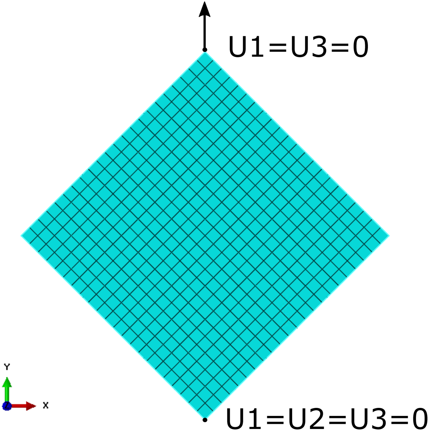

In the experimental work displacements are applied on the picture frame. If this displacement were constant throughout the whole setup there would just be a rigid body motion. Instead, the applied displacement results in a larger actual displacement at the point of load application than more towards the middle of the frame. For this validation, the displacements applied on the edge of the square area of the specimen are calculated and used. These displacements are respectively 0.629, 1.258 and 1.887 mm for displacements applied to the frame of 1, 2 and 3 mm.

The homogenized elastic properties as determined using the RVE should be able to reproduce the results found during the picture frame tests. For the current work the linear approximation of the end-values of the load displacement graph corresponding to displacements of 1–3 mm across three different specimens is compared to the reaction forces in the simulation.

Figure 17 shows the end values for the tension and compression specimens for displacements up to 3 mm. Additionally, it shows the linear approximation for these end values. As has been discussed before the results as presented in Figure 4 and Figure 5 show an initial steep region that is attributed to frame effects. This can also be observed in Figure 17. The relationship between the end values for a specific specimen is linear but if this trend would be extrapolated to displacements of 0 mm the predicted force would be non-zero.

Figure 17.

Linear approximation for end values of load-displacement graphs based on experiments. (a) Compression, (b) Tension.

The numerical model will not be able to predict these frame effects that contribute to the initial steep region. To test whether the simulations can predict the behavior of the fabric their results are compared to end values that do not include the intercept of the linear approximation. Instead, just the slope is used. Figure 18 presents the comparison between these predictions and the simulated end values predicted using both G₁₂ and G₂₁.

Figure 18.

Comparison between linear approximations and simulation for end values.

Figure 18 shows how the load case with G₁₂ results in a simulation that reproduces the response for standard compression specimens very closely. Additionally, it shows that the load case with G₂₁ is not able to accurately predict the actual behavior.

The experimental values for compression and tension specimens for low displacements as shown in Figure 18 are relatively close. Based on these results, the homogenized material properties determined using the RVE with G₁₂ are able to give a good representation of the shear behavior of the fabric for low displacements, regardless of the loading direction.

Discussion

Picture frame tests

Figure 4 and Figure 5 showed a clear difference between the patterns of specimens loaded in tension and compression. Patterns are consistent across multiple specimens. For specimens loaded in compression two clearly different regions are observed while for specimens loaded in tension it is more of a consistent trend.

Creech and Pickett²⁵ present the key mesoscopic fabric deformation mechanisms in a biaxial NCF. From these deformation mechanisms the direction of the stitches influences the shear behavior of the fabric through stitch tension, frictional stitch sliding and interaction between stitching and tows. In the unloaded state of the NCF the stitches are not under tension. The deformation mechanisms of stitch tension and frictional stitch sliding will only become relevant once the stitches are loaded. Up till that point the stitches only contribute through the interaction between stitching and tows. With low displacements the stitches will also not be fully engaged yet, making the stitch-tow interaction the only contribution of the stitches.

The compression results show that there are different mechanisms at play in the reinforcement at different stages of the experiment. Two distinct regions can be defined with a transition where the material becomes significantly stiffer. In the compression case the stitches will not be under tension and will only contribute through the interaction between stitches and tows. However, other deformation mechanisms such as tow compaction, inter-tow shear, inter-tow sliding and cross-over point sliding (as per Creech and Pickett²⁵) will still be present. All mechanisms are subject to coupling and will influence each other.

The compression graphs in Figure 4 and Figure 5 show that the deformation behavior is dependent on the loads that have previously been applied. At the start of the series of experiments the first region with a lower stiffness is short, but as the loads that are applied to the reinforcement become larger so does the length of the first region. The fabric and its behavior have changed over the course of the series of experiments.

It is suggested that in the lower stiffness region inter-tow shear is a dominant deformation mechanism. As the behavior of the fabric changes, the contribution of other deformation mechanisms starts to increase. The test returns the picture frame to the original configuration with no applied displacement or angle after each loading. However, during unloading not all deformation mechanisms will work in a way that returns the fabric to the original configuration. This results in less resistance to shear when the fabric is loaded again until the different deformation mechanisms start to act on the fabric again.

Additionally, as discussed by Colin et al.²⁹ the filament orientation within NCFs is not perfectly aligned with the tow direction. Within tows this can for example include a waviness of the filaments or filaments laying at an angle. For the NCF used in this work filaments have been observed to follow a path from one tow to the neighboring tow between stitching points, thereby travelling a longer path than fibers that are perfectly contained within a single tow. As the fabric is loaded these misalignments will be straightened out, upon unloading they might not go fully back to their origin. This can result in these fibers not being loaded until larger applied displacements.

The tension results show that the stitches are quickly under tension. No obvious differences can be observed in the trend of the graphs for loads from 1 to 10 mm/0.47–4.68°. It would be expected that an obvious increase in stiffness would be observed if the stitches came under tension later in the experiment.Around 0.4–0.5° a small ‘bump’ can be observed in the graphs in the tension graphs in Figure 4 and Figure 5. Since a similar ‘bump’ is present in the reference measurements for an empty frame after testing this is attributed to frame effects.

For the fabric loaded in tension it can also be observed that the fabric changes over the course of the experiment due to the previous loadings. This effect is however less dramatic than for the compression specimens. This is attributed to the stitches playing a large role in the deformation of specimens loaded in tension. The stitches are not largely affected by the loading and unloading of previous experiments in the series.

For this work the end values of the load-displacement graphs are of interest. As shown in Figure 17 the loading direction does not have a large influence on the end-values of standard specimens at displacements of 1–3 mm/angles of 0.47–1.4°. This suggests that at these small displacements and subsequent shear angles the direction of the stitches in the ±45^o bi-axial NCF does not significantly influence the final shearing behavior of the fabric.

For the bi-axial NCF used in this work the maximum allowable fiber angle deviation during handling was found to be 1.4^o. This value is specific to this fabric and cannot be assumed to be valid for other fabrics. The method by which this value has been determined can however be applied to any bi-axial NCF.

No other work has been found that specifically looks at tolerances for the handling process. Gerngross and Nieberl⁴ set a tolerance of ±5^o for picking-up, transporting, draping and positioning of the cut-pieces (dry textile weave or non-crimp fabric). This does however include draping and positioning, which are not considered in the current work.

The method for setting a tolerance for the fiber angle deviations as has been presented in the current work is of value both in designing pick-and-place processes and in monitoring them. Setting a tolerance for fiber angle deviations makes it possible to base design decisions such as pick-up point location on a criterion that directly affects the quality of the final product: the fiber angles. Real-time monitoring becomes most valuable when tolerances are available. Based on these tolerances and feedback from the system decisions can be made on e.g. gripper trajectories, thereby ensuring an optimal the quality of the final product.

Representative volume elements

In the current work periodic RVE homogenization is used to determine homogenized elastic properties for a biaxial NCF. To get from the NCF to the RVE assumptions and simplifications had to be made. As mentioned before the current work assumes that the filaments within a tow are aligned to such an extent that tow angles correspond to filament angles. It does not consider factors such as in-plane waviness as a result of manufacturing. The models are however build up from the tow level, using a series of tows to calibrate the material properties. The mechanical properties for the tows do therefore account for part of the irregularities that might influence bending behavior. Additionally, the results from the RVE were validated using wide fabric strips and picture frame tests.

The algorithm written for this work makes the RVE customizable to a large degree, making it possible to study the influence of for example different stitch patterns on the behavior of the fabric. For now a case study for a single fabric with one specific type of stitch is presented.

The shear moduli of the tows are calibrated by looking at the behavior of the RVE with no stitches present. This has resulted in G₁₂ = G₁₃ = G₂₃ = 0.65 MPa. In real life an NCF without stitches will not have any resistance to shear, this cannot be perfectly represented in simulations. When a sample is clamped in the picture frame and stitches are removed the tows will not remain in their perfectly aligned position. There will be a large loss of contact between tows in the 45^o layer and the -45^o layer and the tows within a layer might also partially lose contact. This results in a large loss of tow-tow interactions that can contribute to the shear resistance. An RVE will always start the simulations with tows perfectly aligned.

However, while an NCF without stitches will not have any resistance to shear, a single tow will. The NCF used in this work is silane treated. This binder does provide additional friction between the tows. Additionally, the friction between the filaments within the tows will contribute to a tows perceived shear modulus. The value of 0.65 MPa for the shear modulus of tows is therefore considered to be reasonable.

The simulated picture frame tests carried out for G₁₂ accurately predicted the end values for compression specimens. G₁₂ simulations should have predicted end values for tension specimens. However, for the region of interest of the current work, end values for compression and tension specimens were close to each other. Due to this observation the RVE is still considered to provide elastic properties that are acceptable to be used in future work.

The values predicted by the simulations with G₂₁ were much lower than found for either compression or tension specimens. As explained before, the trusses in the RVE cannot be loaded in compression. This is similar to how a thread cannot be loaded in compression. However, the experimental results show that compression specimens have a higher resistance to in-plane shear than would be expected. The RVE is a simplified representation of the fabric used in this work. It is suggested that this model is unable to predict the more complex coupling of deformation mechanisms, resulting in an underestimate of the shear resistance.

Conclusions

The present study set out to provide a framework for the determination of acceptable criteria for in-plane shear induced fiber angle deviations in bi-axial non-crimp fabrics. The paper presents a case study for a specific bi-axial non-crimp fabric. For this fabric acceptable criteria are set for the fiber angle deviations and in-plane shear strain. The steps as shown in the current work can be repeated for any bi-axial non-crimp fabric.

The framework and the results that follow from it open up possibilities both for designing pick-and-place processes and for monitoring them. In the design phase the results can aid in making decisions on for example pick-up point placements, the amount of pick-up points and the speed of the process. By simulating the handling process the effect of these process variables on the in-plane shear strain and thus the fiber angle deviations can be observed. Additionally, these simulations can provide the true state of the reinforcement before the fabric is draped or formed. This can then be used as an input for draping or forming simulations. The models required for these simulations are suggested future work based on the current work.

The current results provide a possibility for in-situ monitoring of fiber angle deviations during the pick-and-place process. As long as the in-plane shear strain can be monitored it will be possible to monitor the fiber angle deviations. This can for example provide live feedback on specific handling strategies. It is recommended that future work further investigates the possibilities for this in-situ monitoring.

Footnotes

Acknowledgements

The authors would like to thank D.S. Ruijtenbeek for the support during the mechanical testing of the picture frame tests.

Declaration of conflicting interests

The author(s) declared no potential conflicts of interest with respect to the research, authorship, and/or publication of this article.

Funding

The authors disclosed receipt of the following financial support for the research, authorship, and/or publication of this article: This work was supported by the Aeronautics roadmap by TKI-HTSM, under Grant TKI-HTSM/17.1187.

ORCID iD

Chantal M. de Zeeuw

References

Martinsson

. Development of Robust Automated Handling of Pre Impregnated Carbon Fibre. PhD Thesis. Link¨oping University, 2018.

Kuehnel

Schuster

Buchheim

, et al. Automated Near-Net-Shape Preforming of Carbon Fiber Reinforced Thermo- plastics ( Cfrtp ). In: Innovative composites Summit. Paris, France): JEC Europe, 2014, pp. 11–13.

Krogh

Glud

Jakobsen

, et al. Modeling the robotic manipulation of woven carbon fiber prepreg plies onto double curved molds: A path-dependent problem. J Compos Mater 2019; 53: 2149–2164.

Gerngross

Nieberl

. Automated manufacturing of large, three-dimensional CFRP parts from dry textiles. CEAS Aeronaut J 2016; 7: 241–257.

Mouritz

. Fibre-polymer composites for aerospace structures and engines. In: Introduction to Aerospace Materials. Elsever, 2012, pp. 338–393.

Guzman-Maldonado

Bel

Bloom

, et al. Experimental and numerical analyses of the mechanical behavior during draping of non-orthogonal bi-axial non-crimp fabric composite reinforcements. Mater Des 2022; 218: 110682.

Krieger

Gries

Stapleton

, et al. Shear and drape behavior of non-crimp fabrics based on stitching geometry. Int J Mater Form 2018; 11(5): 593–605.

Wang

Hamila

, et al. Mesoscopic analyses of the draping of 3D woven composite reinforcements based on macroscopic simulations. Compos Struct 2020; 250: 112602.

Krogh

Sherwood

Jakobsen

, et al. Generation of feasible gripper trajectories in automated composite draping by means of optimization. Adv Manuf.: Polym Compos Sci 2019; 5(4): 234–249.

10.

Lin

Clifford

Taylor

, et al. 3D mathematical modelling for robotic pick up of textile components. Compos B Eng 2009; 40: 705–713.

11.

John

Herszberg

, et al. 3D deformation models for the automated manufacture of composite components. Compos A Appl Sci Manuf 2006; 37: 1377–1389.

12.

Ragunathan

Karunamoorthy

. Genetic algorithm-based optimal locations for handling fabric materials in garment automation. Int J Robot Autom 2006; 21(4): 289–294.

13.

Lankalapalli

Eischen

. Optimal pick-up locations for transport and handling of limp materials – Part II: Two-Dimensional Strips. Text Res J 2003; 73: 867–874.

14.

Ballier

. Systematic Gripper Arrangement for a Handling Device in Lightweight Production Processes”, PhD Thesis. Karlsruher Institute of Technology, 2019.

15.

Habboush

Sanbhal

Shao

, et al. Characterization and Analysis of in-plane shear behaviour of glass warp-knitted non-crimp fabrics based on picture frame method. Materials 2018; 11(1550).

16.

Lomov

. Deformability of textile performs in the manufacture of non-crimp fabric composites. In: Lomov

(ed). Non-Crimp Fabric Composites. Cambridge: Woodhead Publishing Limited, 2011, pp. 117–144e.

17.

Fial

Carosella

Ring

, et al. Shear characterization of reinforcement fabrics using textile-applied printed strain sensors. Proced Manuf 2020; 47: 65–70.

18.

Lux

Fial

Schmidt

, et al. Development of a shear forming envelope for carbon fibre non-crimp fabrics. J Ind Text 2021; 15280837211015470.

19.

Santhanakrishnan Balakrishnan

Yellur

Roesch

, et al. Experimental and numerical investigation on draping behaviour of woven carbon fabric. J Ind Text 2021; 15280837211038850.

20.

Drugan

Willis

. A micromechanics-based nonlocal constitutive equation and estimates of representative volume element size for elastic composites. J Mech Phys Sol 1996; 44(4): 497–524.

21.

Omairey

Dunning

Sriramula

, et al. Development of an ABAQUS plugin tool for periodic RVE homogenisation. Eng Comput 2019; 35(2): 567–577.

22.

Lomov

(ed). Non-crimp fabric composites: Manufacturing, properties and applications. Cambridge: Woodhead Publishing Limited, 2011.

23.

Long

Souter

Robitaille

, et al. Effects of fibre architecture on reinforcement fabric deformation. Plast Rubber Compos 2002; 31(2): 87–97.

24.

G´omez

Ram´on

Torregaray

, et al. Mechanical behaviour of thermoplastic (pes, pbt) carbon nanofibre composites. ICCM 2009; 17.

25.

Creech

Pickett

. Meso-modelling of Non-crimp Fabric composites for coupled drape and failure analysis. J Mater Sci 2006; 41: 6725–6736.

26.

Pabst

Krzywinski

Schenk

, et al. Seams and Bending in Cloth Simulation,” Workshop in Virtual Reality Interactions and Physical Simulation VRIPHYS, 2008.

27.

Döbrich

Gereke

Diestel

, et al. Decoupling the bending behavior and the membrane properties of finite shell elements for a correct description of the mechanical behavior of textiles with a laminate formulation. J Ind Text 2014; 40(1): 70–84.

28.