Sage Journals: Discover world-class research

Abstract

Control and optimization of coaxial electrospinning process is a serious concern due to its multiparameter effectiveness. This study is concerned with modeling and simulation of process by solving the governing equations of electrified jet using FEniCS software packages applying Cahn–Hilliard and Newton solvers for finite element method. Jet diameter, solvent evaporation, electrical field, and velocity changes are focused in this model as the most effective parameters on final nanostructures quality. An experimental core–shell nanofiber production (polyvinyl alcohol) in the same spinning condition with simulated spinning is applied to validate the model. Both theoretical and experimental results demonstrate that core and shell diameter increases by increase in nozzle diameter and polymer solution concentration. Relative error shows that for the higher nozzle diameter, the model can have an acceptable prediction for final diameter which is more accurate for shell diameter part. The simulation results for jet velocity indicate a sharp sinusoidal increase during jet motion. Electric field simulation also shows a result similar to Feng’s model with an increase near the nozzle and a very slow decline at the end which both are confirmed by other experimental and numerical studies. It is also concluded that by enlargement of nozzle diameter, solvent evaporation takes more time and as a result, the inhomogeneity and diameter increase which have the same trend as experimental results. The relative error of evaporation time decreases in nanojets with higher diameter. And the model has an acceptable compatibility with experimental results especially for nozzle diameters more than 50 µm.

Keywords

Modeling and simulation newton solver solvent evaporation core–shell nanofibers fiber diameter

Introduction

Electrospinning is an established nano industrialized technology producing continuous nanofibers from polymer solutions in high electric fields [1 –4]. Due to the very high aspect ratio, specific surface area, flexibility in surface functionalities, and superior mechanical properties of electrospun nanofibers, many investigations have been done in using them for a variety of applications including drug delivery [5], tissue engineering [5,6], conductive nanowires [7], nanosensors [8], biochemical protective clothing for the military [9], wound dressing [10], and templates for nanotubes [11]. Currently, nanofibers and nanostructures comprising single or blended materials have been widely produced [12,13].

Coaxial electrospinning for core–shell micro and nanofibers production was introduced in the last decade as a branch of nanotechnology, which their applications are being explored and developed in biotechnology, drug delivery, and nanofluidics [14 –17].

Coaxial electrospinning was first demonstrated by Sun et al. [14] and after that, Li and Xia [18] used coaxial electrospinning to produce TiO₂ hollow nanofibers with controllable dimensions. In a coaxial electrospinning setup, a dual syringe with two compartments containing different polymer solutions or a polymer solution (shell) and a non-polymeric Newtonian liquid or even a powder (core) is used to initiate a core–shell jet. At the exit of the core–shell needle attached to the syringe appears a core–shell droplet, which acquires a shape similar to the Taylor cone due to the pulling action of the electric Maxwell stresses acting on the fluid. Core–shell cone is subjected to sufficiently strong electric field, issues a compound jet, which undergoes the electrically driven bending instability characteristic of the ordinary electrospinning process which is coincided with jet thinning and fast solvent evaporation. As a result, the core–shell jet solidifies and core–shell fibers are depositing on the collector [19 –21].

Core–shell nanofibers have been the subject of many studies because of their unique properties such as high length-to-diameter ratio, potential to cover unspinnable materials, using as continuous nanotubes in hollow form. Potential application in biomedical areas such as preserving an unstable biological agent from an aggressive environment, preventing the decomposition of a labile compound under a certain condition, delivering a biomolecular drug in a sustained way, and functionalizing the surface of nanostructures without affecting the core material attracts many attentions to these kinds of nanofibers [5,22 –27].

The novelty of coaxial electrospinning lies in that coaxial two liquid nanojets which consist of a shell-forming liquid on the outer side and an inert (probably immiscible) liquid on the inner side, the latter constituting a very broad and general family of liquid nanotubular templates requiring no molecular-level assembly [14,28 –30]. Similar to simple electrospinning, in this technique, electrohydrodynamic forces cause meniscus exiting from the tip of a capillary, when subject to an appropriate electric field, and deforming into a conical shape (Taylor cone) [3]. The jet generally desires to break up into a spray of highly charged nanodroplets, named “electrospray,” unless the jet solidifies before such physical natural disruption occurs [31 –33]. According to this fact, solvent evaporation plays a critical role in nanofiber and core–shell nanofibers formation. Rapid solvent evaporation accompanied by jet stretching due to electric forces and jet instabilities is ultimately responsible for the diameter, structure, and properties of the final solidified nanofibers and core–shell nanofibers [34,35].

Several theoretical investigations about different aspects of coaxial electrospinning and electrospraying with the goal of process efficiency enhancement and well understanding of its underlying physics have been done so far by trying to control effective parameters including solution parameters in terms of concentration and the process parameters such as flow rate, applied voltage, and nozzle tip–collector distance [36 –41]. But there are few studies concerning coaxial electrospinning modeling and simulation for core–shell or hollow nanofibers morphology optimization and control since most of them focused on drug delivery modeling or biomedical science [42,43]. Herráez et al. [44] modeled the cross section of component nanofibers to optimize uniformity and random dispersions and tensile thermal residual stresses while they did not focus on spinning procedure modeling and other parameters such as diameter, electric field, jet velocity, and solvent evaporation as our model.

Pokuri and Ganapathysubramanian [45] modeled specifically blend ratio and evaporation rates during production process of blend fibers (not exclusively symmetric compound nanofibers such as core–shell ones which has vast applications). These works also have a lack on studying core–shell nanojets morphology and behavior and other essential parameters that are included in our work. Du and Chaudhuri [46] operate a computational multiphysics model for simulating the formation and breakup of droplets from axisymmetric charged liquid jets in electric fields. They did not work on micro or nano scale and they just focus on droplet behavior not fiber form. Extra morphological information is missed and like previous works there is no experimental works to validate the model. Wang et al. [39] assess the influence of different coaxial composite nozzle structures on Taylor cone shape and electric field intensity distribution was studied by ANSYS finite element simulation method. They also validated their model by experimental data but they did not focus on jet motion modeling, behavior, and morphology such as diameter and solvent evaporation changes during process.

However, there is still no adequate entirely mathematical and physical theory for electrically driven, viscoelastic core–shell jets similar to other technologies [39,47,48]. A novel model is introduced in this research to optimize this valuable technique. In discussed model we have six governing equations (mass, momentum conservation, Maxwell and Fick’s equations together with the advection–diffusion equation of the diffuse interface for electrified fluid jet) which solved more unknown parameters than previous studies. We obtained core and shell diameters theoretically and experimentally while the effect of nozzle diameter and polymer solution concentration is assessed on them. In addition, we simulate coaxial jet velocity and electric field during its motion toward the collector which is validated with previous numerical works. On the other hand, solvent evaporation rate, the resulted inhomogeneity, total time of solvent evaporation, and its relation with diameter are simulated and discussed too. Experimental spinning process in the same condition with simulation virtual setup has been done to validate the model. Furthermore, we apply FEniCS package software that works under python language which is more new, fast, and user friendly than other applied software and languages in previous numerical investigations.

Numerical method

In this study, a new method based on Cahn–Hilliard equation was applied to model coaxial electrospinning process in order to superior control of electrospun nano jet by applying FEniCS package software. The Cahn–Hilliard equation is a parabolic equation and is typically used to model phase separation in binary mixtures. Many important industrial problems involve flows with multiple constitutive components such as fabrication of core–shell nanofibers [14], bubbly and slug flows in a microtube [49], and drop coalescence and retraction in viscoelastic fluids [50]. Due to inherent nonlinearities, topological changes, and the complexity of dealing with unknown moving interfaces, multiphase flows are challenging to study from mathematical modeling and numerical algorithmic points of view [51,52].

Phase-field models are an increasingly popular choice for modeling the motion of multiphase fluids to have more accurate and acceptable results. The basic idea is to introduce a conserved order parameter such as a mass concentration that varies continuously over thin interfacial layers [53]. In the phase-field model, sharp fluid interfaces are replaced by nonzero thin thickness transition regions where the interfacial forces are smoothly distributed as it is applied in discussed model to have more accurate theoretical data. The total domain and the boundary of interface are denoted by Ω and Γ. The unit outward normal to Γ is denoted as n. We assume the boundary Γ is composed of two complementary parts, Γ = Γ_g + Γ_s. Figure 1 shows schematic diagram of a two-phase domain. The evolution of the mixture is assumed governed by the Cahn–Hilliard equation and the problem can be stated as (equation (1) is the main equation of phase-field method, equations (2) to (5) are boundary and initial conditions, respectively)

\frac{\partial φ}{\partial t} = \nabla . (M_{φ} \nabla (μ_{φ} - λ Δ φ)) in Ω \times (0, T)

(1)

φ = g on Γ_{g} \times (0, T)

(2)

M_{φ} \nabla (μ_{φ} - λ Δ φ) . n = s on Γ_{s} \times (0, T)

(3)

M_{φ} (λ \nabla φ) . n = 0 on Γ \times (0, T)

(4)

φ (x, 0) = φ_{0} (x) in Ω

(5)

where M_ϕ is the mobility, μ_ϕ represents the chemical potential of a regular solution in the absence of phase interfaces, and λ is a positive constant (chemical potential which is considered to be 0.5 commonly) such that √λ is considered as the thickness of the interfaces that represents the transition between the two phases [54,55]. In the most of analytical studies, the mobility is a function of order parameter (ϕ) [54]

M_{φ} = K φ (1 - φ)

(6)

where K is a positive constant (0 < K < 1).

Figure 1.

Schematic diagram of a two-phase domain.

The function μ_ϕ is a nonlinear function of the order parameter (ϕ). It is usually approximated by a polynomial of degree three. In this paper, we consider the thermodynamically consistent function, namely

μ_{φ} = \frac{1}{2 θ} \log \frac{φ}{1 - φ} + 1 - 2 φ

(7)

θ is a function of temperature that following [54], we will take the value θ = 3/2 for that.

Solvent evaporation rate can be calculated according to Fick’s law. Mass conservation of the mixture requires $c_{1} \bar{V_{1}} + c_{2} \bar{V_{2}} = 1$ . The axisymmetric Fick’s law of mass diffusion in the radial direction gives (where c₁, c₂, $\bar{V_{1}}$ and $\bar{V_{2}}$ are the mass concentrations, specific partial volumes of the mixture, respectively)

J_{i} = \frac{{Dc}_{i}}{RT} \nabla η_{i}

(8)

J_{i} = D \frac{\partial c_{i}}{\partial r}

(9)

where J is the “diffusion flux” of which the dimension is the amount of substance per unit area per unit time, so it is expressed in such units as mol/m² s. Diffusion flux measures the amount of substance that will flow through a unit area during a unit time interval. D is the diffusion coefficient or diffusivity. Its dimension is area per unit time, so typical units for expressing would be m²/s. The index i denotes the ith species, c is the concentration, R is the universal gas constant (8.3144 J/K/mol), T is the absolute temperature of spinning chamber (25℃ = 298.15 K), and η is the chemical potential (J/mol). So, it can be written as

\frac{\partial c_{i}}{\partial t} = \frac{\partial}{\partial r} (J_{i})

(10)

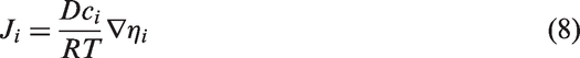
Using initial and boundary condition, jet diameter and solvent evaporation parameters are related as below

r = R (t) : \frac{dR (t)}{dt} = - \frac{k_{g} M_{si}}{RT ρ_{si}} (p_{s i} - p_{\infty})

(11)

where R(t) is the jet radius in time t; k_g (cm/g) is the coefficient of solvent mass transfer at the jet surface; M_si is the solvent molar weight for both core and shell solutions (M_s₁ and M_s₂ are solvent molar weight for shell and core solution, respectively); T is the absolute temperature near the surface; R = 8.3144 J/mol is the universal gas constant; p_∞ is the solvent vapor pressure in the atmosphere far from the jet surface (p in this study); p_si is the solvent saturation vapor pressure near the jet surface or interface for both core and shell solutions (p_s₁ and p_s₂ are the vapor pressure for shell and core solution respectively); and ρ_si is the solvent density of both parts as well (more explanation in given in Appendix 1) [34,56].

The parameters used in this simulation, concerning Fick’s equation, the same as experimental part, are as follows:

The mass densities of solvent for according to Polyvinyl alcohol (PVA)/water solution in shell and water in core part (M_s₁ = 18 and M_s₂ = 18) are ρ_s₁ = 1 g/cm³ and ρ_s₂ = 1 g/cm³ (solvent is water in both solutions in this case). The PVA diffusion coefficient in infinite water is D = 0.2 × 10⁻⁴ m²/s [57] (Appendix 1 formulas). Solvent (water) saturation vapor pressure at 25℃ is for both core and shell solution is considered as p_s₁ and p_s₂= 3170 Pa [58]. The solvent mass transfer coefficient at the jet surface is k_gi which are k_g₁= 0.90 × l0⁻³cm/s for water in PVA/water solution in shell part and k_g₂ = 1.8 × 10⁻³ for water in shell part, by analogy with similar solvents [59].

So equation (11) can be written as

\frac{dR (t)}{dt} = - \frac{k_{g} M_{si}}{RT ρ_{si}} (p_{si} - p)

(12)

In this approach a set of governing equations, which are used for coaxial jet motion modeling, are contained mass and momentum conservation, Maxwell and Fick's equations for fluids together with the advection–diffusion equation of the diffuse interface are used to solve as following:

\nabla . u = 0

(13)

ρ (\frac{\partial u}{\partial t} + u . \nabla u) = - \nabla . p - \frac{1}{2} E . E \nabla ɛ + \nabla . (ɛ E) E + \nabla . η (\nabla u + \nabla u^{T})

(14)

\nabla . (ɛ_{r} E) = ρ_{e}

(15)

\nabla \times E = 0

(16)

\frac{\partial φ}{\partial t} + \nabla . (φ u) = - \nabla . [- Γ (φ) \nabla λ] = \nabla . (M_{φ} \nabla λ)

(17)

\frac{dR (t)}{dt} = - \frac{k_{g} M_{Si}}{RT ρ_{si}} (p_{si} - p)

(18)

where u, t, ρ, p, η, g, ϕ, λ, ɛ_r, E, and ρ_e denote velocity, time, density, pressure tensor, viscosity, gravity, order parameter (in Cahn–Hilliard method), chemical potential, relative dielectric constant, electric field, and volumetric charge density, respectively [60]. Relative dielectric constant ɛ can be obtained by

ɛ_{r} = \frac{ɛ_{f 1}}{ɛ_{f 2}}

(19)

where ɛ_f₁ and ɛ_f₂ are dielectric constants of the first and the second fluid, respectively.

According to equation (18) the diameter of shell and core parts of nanojet can be calculated for each time step by inserting M_s₁, p_s₁, and ρ_s₁ constants for the shell and M_s₂, p_s₂, and ρ_s₂ constants for the core parts of nanojets. Furthermore, p is calculated from other mentioned governing equations in the discussed partial differential equations system (as it can be seen in Figure 2 and Table 1 in “Results and discussion” section). On the other hand, equation (17) is for one time step. Total time steps, which used to complete solving equations, is applied as theoretical solvent evaporation time.

Figure 2.

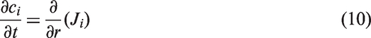
Coaxial electrospinning setup.

Table 1.

Comparison between theoretical and experimental nanofiber diameter in different initial jet diameter (nozzle diameter) and polymer solution concentration for both core and shell part of nanofibers (spinning distance is considered to be 10 cm).

Initial jet diameter (µm)	Polymer solution concentration (wt%)	Theoretical shell diameter (µm)	Theoretical core diameter (µm)	Experimental shell diameter (µm)	Experimental core diameter (µm)	Shell diameter relative error (%)	Core diameter relative error (%)
10	6	0.54	0.32	0.49–0.63	0.28–0.42	3.7	9.0
30	6	1.29	0.76	0.70–1.92	0.42–1.22	2.0	6.0
50	6	1.82	0.98	1.35–2.23	0.56–1.31	1.0	2.5
10	10	1.21	0.73	0.72–1.75	0.37–1.18	2.0	6.0
30	10	1.57	1.06	1.07–2.11	0.67–1.52	1.2	3.0
50	10	1.83	1.29	1.44–2.24	0.78–1.77	0.5	1.0

Experimental

The PVA (Mw = 72,000 Da) was obtained from Merck Company and its solution was prepared by dissolving PVA in deionized water for shell part of nanofibers. The solution was magnetically stirred at 80℃ for 2 h to obtain homogenous solution. Coaxial electrospinning was performed in two different concentrations of PVA/water (6 and 10%) and distilled water for core part of nanofibers. Five different size of syringes (with diameter of 10, 30, 50, 70, and 100 µm) was placed on a programmable syringe pumps for both shell and core fluid, respectively. The initial spinning condition for experimental section is adjusted similar to the simulation part in order to provide better comparison situation between experimental and theoretical data. Spinning distance, ambient temperature, initial voltage, nozzle diameter (initial jet diameter), and flow rate in experimental spinning setup are selected as 10 cm, 25℃, 0 V, 10–100 µm, and 0.1 ml/h, respectively. Figure 2 shows the structure of coaxial electrospinning setup.

Scanning electron microscope (Philips XL-30) was employed to get and control nanofiber diameters. Further diameter characterization was applied for core–shell electrospun nanofibers using JEOL JEM-2010F FasTEM field emission electron microscope operated at 100 keV in order to measure core and shell part of nanofibers separately and to compare with simulation results. The samples were dried in a vacuum oven for 48 h at room temperature prior to TEM imaging. Typical SEM and TEM images of electrospuned core–shell PVA nanofibers are shown in Figures 4 and 5.

A high-speed video camera and the TAG Heuer Mikrotimer Flying 1000 that can track time down to 1/1000th of a second is applied to measure very fast motion of coaxial jet to compare with theoretical solvent evaporation time. The total time for the fluid jet motion toward the collector is considered as experimental evaporation time because solvent evaporation completed when the solid electrospuned nanofibers lay out on the collector.

Results and discussion

Discussed governing nonlinear equations (13) to (18) have been solved in a partial differential equations system simultaneously applying FEniCS package software in every time steps and grids of defined finite element mesh. The virtual setup frame in this modeling is defined in a way that spinning distance and the nozzle dimensions are simulated to be as same as the real operating coaxial electrospinning setup. Final results such as jet’s diameter in core and shell part, velocity profile, electric field magnitude, and solvent evaporation rate are defined for every time steps and grids of finite element mesh which are analyzed using Paraview software. Figure 3 depicts simulation results of core–shell nanofiber’s jet diameter changes under electric fields.

Figure 3.

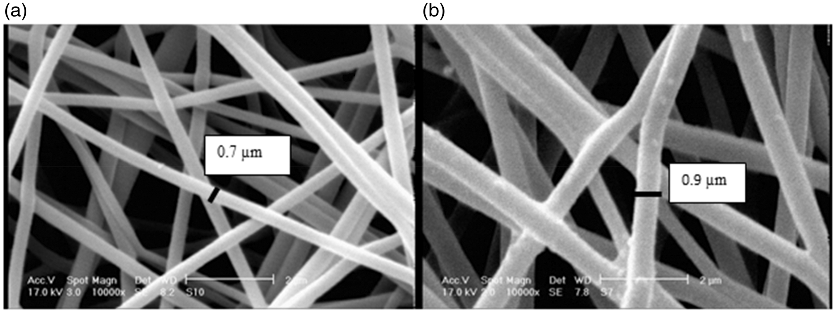
Theoretical results of jet diameter changes during motion toward collector using FEniCS simulation are presented: (a) Taylor cone creation, (b) jet initiation, (c) jet motion toward collector, (d) arriving to the collector, (e) core and shell diameter changes during coaxial electrospinning (nozzle diameter, spinning distances, and solution concentration are considered to be as 50 µm, 10 cm, and 6%, respectively).

Figure 4.

TEM results of PVA/water core–shell nanofibers with different polymer solution concentration: (a) polymer concentration of 10% and (b) polymer concentration of 6%. (Other spinning parameters such as nozzle diameter, spinning distances, temperature, initial voltage, and flow rate are selected as 50 µm, 10 cm, 25℃, 0 V, and 0.1 ml/h for both samples, respectively.) PVA: Polyvinyl alcohol; TEM: Transmission electron microscopy.

Figure 5.

SEM results for PVA core–shell nanofibers with different polymer solution concentration: (a) polymer concentration of 6% and (b) polymer concentration of 10%. (Other spinning parameters such as nozzle diameter, spinning distances, temperature, initial voltage, and flow rate are selected as 50 µm, 10 cm, 25℃, 0 V, and 0.1 ml/h for both samples, respectively.) PVA: Polyvinyl alcohol; SEM: Transmission electron microscopy.

The continuous and dotted lines show core and core–shell diameter changes during coaxial electrospinning, respectively. The initial diameter of core–shell jet and as a consequence core–shell nanofiber is considered equal to the electrospinning nozzle diameter. As it is recognized in the graph, the diameter reduction of the jet is sharply at first and slowly at the end of the process. At the initial stages of the process, the jet is coming out of the electrospinning nozzle as a drop named Taylor cone [36,43,61]. Finally a jet diameter reduction is obvious in the last part of simulation which is similar to other theoretical study results [33,62,63]. The primary jet is exerted toward collector because of attraction force between electrode connected to the collector and surface electric charges on coaxial jet. Although the force of polymer’s viscosity and surface tension resists against the movement of fluidic jet, the electric force between two electrodes can overcome these forces if the voltage magnitude is selected correctly. As it can be seen from the vortexes around the jet, velocity is increasing during the process and the jet is further accelerated by the time. It is clear from Figure 3 that jet diameter of both phases is decreased, which is consistent with Feng’s model [62].

The diameter reduction occurs during electrospinning mostly at first and middle of jet motion and slowly at the end, which can be considered as core–shell nanofiber diameter. According to this analytical model, forces that determine the jet diameter during electrospinning or coaxial electrospinning can be considered as of viscosity, surface tension, electric force, and flow rate which all influence jet velocity [15,64,65]. Electric field and diameter changes are deeply interrelated. Since the jet becomes thinner downstream, the increasing of jet speed enlarges the surface charge density and thus electric field which creates electrostatic forces. The produced electric force exerts on the jet and thus diameter becomes smaller [62]. Figure 4 shows TEM photographs of PVA core–shell nanofibers with the same spinning parameters with simulation setup, such as flow rate, voltage, nozzle diameter, spinning distance, and different polymer solution concentration (6 and 10%). As it is obvious, reduction of the concentration is leading to the finer nanofibers. Sharp boundaries of core–shell structure can be clearly seen along the nanofiber length which indicates well produced and homogenous core–shell nanofibers.

Figure 5 presents SEM photographs of PVA core–shell nanofibers with the same spinning parameters with simulation setup. The reduction of nanofibers diameter in more dilute polymer solution is clear in these photographs too. These experimental results are compared with the designed simulation in the following.

Table 1 signifies a comparison between theoretical and experimental nanofiber diameters in different initial jet diameter (nozzle diameter) for both polymer solution concentration (6 and 10 wt%) with spinning distance of 10 cm for both shell and core parts of nanofibers. It can be found that the model results have good compatibility with the experimental data with the same initial parameters including flow rate, applied voltage, solution concentration, and nozzle diameter. The two data in experimental columns for both core and shell parts (in this section, shell diameter is related to the total diameter of the nanofiber) indicate the minimum and maximum amount of measured diameter. Since naturally there are inhomogeneities in final diameter of collected nanofiber, the average diameter for both core and shell part is considered in calculating relative error (RE) between experimental (Diameter_e) and theoretical (Diameter_t) data due to the following equation

RE = \frac{D_{e} - D_{t}}{D_{t}} \times 100

(20)

where D_e and D_t are experimental and theoretical diameters, respectively.

In order to have a reliable average diameter, for each spinning condition (discussed different nozzle diameters and polymer solution concentrations), 50 different points of nanofibers are selected randomly to measure their diameter applying their SEM and TEM photographs for both core and shell parts. The average diameter is calculated by adding all selected sample diameters divided by 50 for both parts.

RE values that are used for comparing theoretical and experimental results in this table (and also Table 2) can demonstrate the compatibility and validity of this model. On the other hand, the model can help future researches to use diameter simulation and select the spinning condition with less RE before experimental or even industrial nanofiber production in order to save time and budget. In Table 1, RE shows that for the higher nozzle diameter (coarser nanofibers) and higher polymer solution concentration, the model can have an acceptable prediction for core and shell diameter of nanofibers. Furthermore, RE is less in shell diameter (total diameter of nanofiber) measurement rather than core part and can be used confidently for predicting nanofiber diameter in all polymer solution concentration before experimental produce. In addition, for nozzle diameter of 30 and 50 µm, especially in higher polymer solution concentration, a reliable prediction is possible for core diameter according to theoretical results. Most of the theoretical works in this field did not consider nanofiber diameter changes or did not report its compatibility with experimental results [4,63,66]. Among few works that focused on these significant parameters, this model is more reliable due to less RE [67].

Table 2.

Variation in the jet drying time (solvent evaporation time) with the initial jet diameter.

Initial jet diameter (µm)	Polymer solution concentration (wt%)	Theoretical evaporation time (s)	Experimental evaporation time (s)	Theoretical shell diameter (µm)	Experimental final diameter (µm)	Evaporation time relative error (%)
10	6	0.0014	0.001	0.54	0.60–0.78	28.2
30	6	0.0090	0.010	1.29	0.70–2.08	11.1
50	6	0.0125	0.034	1.82	1.35–2.23	4.6
70	6	0.2280	0.233	2.09	1.56–2.61	2.1
100	6	0.3120	0.310	2.51	1.88–3.11	0.6
10	10	0.0123	0.012	1.21	0.72–1.75	24.3
30	10	0.0940	0.103	1.57	1.07–2.11	9.5
50	10	0.2400	0.233	1.83	1.44–2.24	2.9
70	10	0.5700	0.560	2.48	2.23–2.55	1.7
100	10	0.8730	0.875	2.87	2.37–3.02	0.2

Figure 6 shows coaxial jet velocity and electric field changing during coaxial electrospinning. As clearly seen, velocity increases like a sinusoidal equation during coaxial electrospinning process that is similar to some related models [68,69]. At the initial stage jet velocity depends on the electric force between two electrodes of system profoundly. Since the electric force is small at the first time steps, surface tension and viscosity forces resist jet movement. Hence, the velocity increase is slow. After thinning the jet in the middle of the process, surface charge density and as a result electric force increases in a way that they can dominate opposition forces. Therefore, the jet velocity and as a result electric field has a sharp rise. Electric field increases in the jet motion direction and will lead to a huge electric force which accelerates the coaxial jet toward the collector. It has a maximum value after passing the nozzle since the shrinking diameter of the jet in combination with charge conservation demands a higher rate of convection, leading to surface charge density, ρ_e, growing [33,43,70]. As the jet becomes thinner downstream, the velocity increases and electric field decreases slowly after a sharp rise which is confirmed by Feng model [62,63].

Figure 6.

Jet velocity and electric field magnitude increase in coaxial electrospinning process.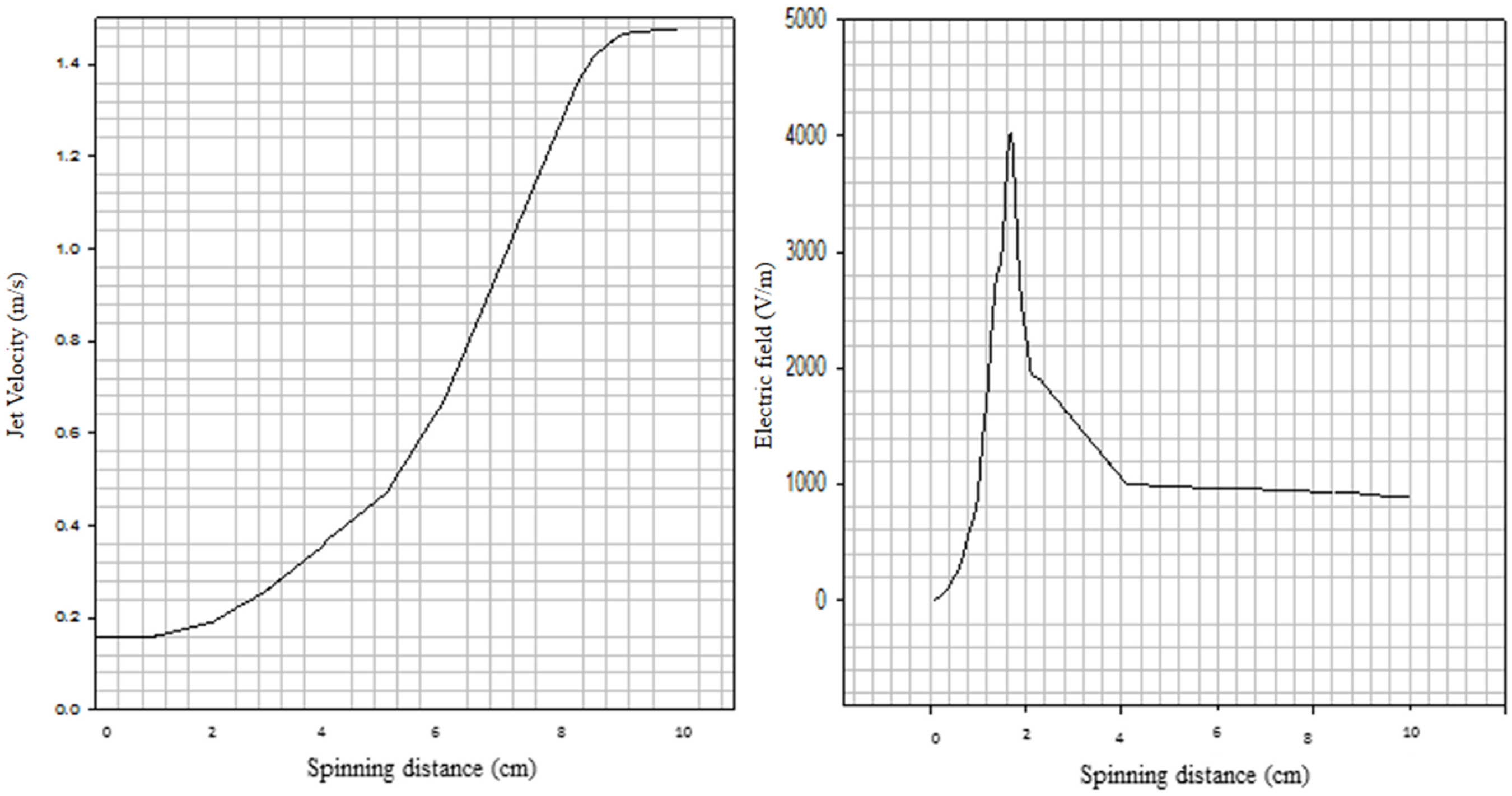

As mentioned before, solvent evaporation plays a critical role in nanofiber formation and jet diameter changes in electrospinning and coaxial electrospinning. Applying Fick’s law, the following assumptions are used in this model to simulate solvent evaporation from thin polymer jets: (a) no temperature gradient exists inside the jet, (b) the mass diffusion and transfer is axisymmetric, and (c) no chemical reactions take place inside the jet [34,35,71].

Figure 7 depicts solvent evaporation trends with different nozzles. According to the figure, at the first stages of the spinning process, the amount of evaporated solvent is more and during jet motion, it decreases. It is an expected trend because by passing the time, less solvent will be remained to be evaporated (as it is approved in Figure 8 too).

Figure 7.

Simulation of core–shell jet solvent evaporation in a virtual electrospinning setup using FEniCS model with nozzle diameter of (a) 50 µm and (b) 10 µm, respectively. (Polymer solution concentration, time of process, and spinning distances for both nozzle diameters setup are considered to be 10%, 10 ms, and 10 cm respectively.)

Figure 8.

Solvent evaporation rate in different polymer solution concentration. (Polymer solution concentration, spinning distances, and nozzle diameters setup are considered to be 6–10%, 10 cm, and 50 µm, respectively.)

On the other hand, numerical simulation demonstrates high transient inhomogeneity of solvent concentration evaporation on the surface of the spinning jet. The degree of inhomogeneity decreases when the spinning jet becomes finer as it is shown in Figure 7. It means that the jet with lower nozzle diameter is more homogeneous. The simulated jet drying time decreases rapidly with the decreasing initial jet diameter as it has good compatibility with experimental data. Solving Fick’s governing equation by different initial nozzle diameter (initial jet diameter) leads to various solvent evaporation times which show some extent of homogeneity.

Table 2 shows the variation of evaporation time of the solvent with the initial jet diameter (nozzle diameter). The data present that by increasing the diameter of the nozzle, solvent evaporation takes more time and as a result, there will be more inhomogeneity and larger diameter which has the same trend as experimental results. On the other hand, according to both theoretical and experimental results, solvent evaporation time becomes larger by increasing the concentration from 6 to 10%, in Table 2. Relative error percentage for evaporation time is calculated as following to have a comparison between experimental and theoretical data

RE = \frac{t_{e} - t_{t}}{t_{t}} \times 100

(21)

where t_e and t_t are experimental and theoretical evaporation times, respectively.

As discussed previously, relative error values can compare theoretical and experimental results precisely to confirm validity of the model. By applying a simulated virtual electrospinning setup before operating, nanofibers manufactures can have faster and less expensive production procedure. As mentioned before, the total time for the fluid jet motion toward the collector is estimated as experimental evaporation time, that is discussed in this section, because solvent evaporation completed when the solid electrospuned nanofibers lay out on the collector.

As it is obvious, evaporation time relative error percent decreases in coarser nanojets. It means that when the initial nanofiber diameter increases, the model has an acceptable compatibility with experimental results especially for nozzle diameters more than 50 µm.

For the electrospun nanojets with initial diameter of 30 µm and less, jets motion is extremely fast and even experimental measurements of the time still have errors despite many repetitions. Because of that the relative error is reasonably high. But for coarser nanojets, this model can apply to predict the evaporation time acceptably. The amount of relative error percentage is less for nanofibers with more concentrated polymer solution and the best result for prediction solvent evaporation time is nanofibers with nozzle diameter and polymer solution concentration of 100 µm and 10 wt%, respectively.

A comparative plot of solvent evaporation rates for different polymer solutions (6 and 10 wt%) containing PVA and water is presented in Figure 8. Spinning distances and nozzle diameters setup are considered to be 10 cm and 50 µm for both polymer solution concentrations, respectively. By increasing polymer solution concentration from 6 to 10%, evaporation time increases because the solution evaporation procedure is easier in more dilute solution. This fact affects final diameter of nanofibers while in the equal spinning distance, solvent evaporation rate increases in more dilute polymer solution leading to finer nanofibers as it can be compared in Table 2. The evaporation rates are calculated from the slope of evaporation curves for the mentioned solutions which is higher for 6% polymer solution obviously.

Conclusion and outlook

Development of coaxial electrospinning technologies for industrial applications should probably be more challenging than in the case of an ordinary electrospinning due to the multiphysical nature of the process and the complex interplay of multiple design, process, and material parameters. Being basically a simple and economical process, coaxial electrospinning can have large-scale industrial future by devoting more attention to physical phenomena which govern coaxial jet and as a consequence resultant core–shell nanofibers. This strategy will avoid unnecessary costs, reducing trial-and-error campaigns leading to fast material developments for tailored properties.

This study has focused on modeling and simulation of coaxial electrospinning by focusing on solving the governing equations of mass, momentum conservation, Maxwell and Fick’s equations together with the advection–diffusion equation of the diffuse interface for electrified fluid jet using software packages including FEniCS, GMSH, and Paraview software by applying Cahn–Hilliard and Newton solvers for finite element method.

Simulation results indicate that diameter reduction for both core and shell parts, occur mostly at first and middle of jet motion and slowly at the end of the electrospinning process. Applying this analytical model, nanofiber diameter for both core and shell parts with different polymer solution concentration (6 and 10%) and nozzle diameter (10, 30, and 50 µm) with the equal spinning distances of 10 cm were calculated and compared with experimental results in the same spinning condition.

Calculated relative error shows that for the higher nozzle diameter and polymer solution concentration, the model can have an acceptable prediction for core and shell diameter of nanofibers. Furthermore, relative error is less in shell diameter (total diameter of nanofiber) measurement rather than core part, but in initial nanofiber diameter of 30 and 50 µm, especially in higher polymer solution concentration, theoretical results can be used for core diameter prediction justifiably. On the other hand, TEM and SEM results for experimentally produced core–shell PVA nanofibers confirmed that both core and shell diameter decrease in more dilute polymer solution.

Modeling and simulation results for jet velocity and electric field are depicted in this model. Numerical results represent a sharp sinusoidal increase during jet motion toward collector for all spinning conditions which is confirmed by other experimental and numerical studies. As the jet becomes thinner downstream, the velocity increases and electric field decreases slowly after a sharp rise which is confirmed by Feng model. The velocity of electrified jet and resulted electric force magnitude changes are deeply related to each other. The reason is that increasing electric field, the surface charge density and as a result electric force is necessary to dominate opposition forces against jet motion in order to accelerate the jet. Therefore, electric field increases in the jet motion direction, leading to a huge electric force which accelerates the jet toward the collector with high velocity.

Investigation of the solvent evaporation behavior of the process by mentioned model indicates that by nozzle diameter increasing, solvent evaporation takes more time and as a result, there will be more inhomogeneity which has the same trend as experimental results. Furthermore, simulation results exhibit that more concentrated polymer solution jet needs more time to be dried. The evaporation rates can be calculated from the slope of evaporation curves for the different polymer solutions which is higher for 6% polymer solution obviously. Evaporation time relative error percent decreases in nanojets with higher diameter. And the model has an acceptable compatibility with experimental results especially for nozzle diameters more than 50 µm. The best result for prediction solvent evaporation time is nanofibers with nozzle diameter and polymer solution concentration of 100 µm and 10 wt%, respectively.

Regarding to discussed results, this model can successfully help future researchers to apply related virtual setup simulation for different parameters to select the spinning condition with less relative error before moving to the nanofiber manufacturing sector in order to save time and budget.

Footnotes

Declaration of Conflicting Interests

The author(s) declared no potential conflicts of interest with respect to the research, authorship, and/or publication of this article.

Funding

The author(s) received no financial support for the research, authorship, and/or publication of this article.

Appendix 1

References

Bhardwaj

Kundu

. Electrospinning: A fascinating fiber fabrication technique. Biotechnol Adv 2010; 28: 325–347.

Fong H and Reneker DH. Electrospinning and the formation of nanofibers. Structure formation in polymeric fibers. Vol. 6. Hanser, Cincinnati, USA: Hanser Gardner Publications, 2001, p.577.

Taylor G (ed) Electrically driven jets. Proc R Soc Lond A Math Phys Eng Sci 1969; 313: 454–483.

Mohammadzadeh moghadam

Dong

Davies

. Modelling electrospun nanofibers: An overview from theoretical, empirical, and numerical approaches. Int J Polym Mater 2016; 65: 901–915.

Sill

von Recum

. Electrospinning: Applications in drug delivery and tissue engineering. Biomaterials 2008; 29: 1989–2006.

Pham

Sharma

Mikos

. Electrospinning of polymeric nanofibers for tissue engineering applications: A review. Tissue Eng 2006; 12: 1197–1211.

Xia

Wei

Wan

. Conducting polymer nanostructures and their application in biosensors. J Colloid Interface Sci 2010; 341: 1–11.

Zhang

Zheng

et al.

Highly sensitive and stable humidity nanosensors based on LiCl doped TiO₂ electrospun nanofibers. J Am Chem Soc 2008; 130: 5036–5037.

Graham K, Gogins M and Schreuder-Gibson H (eds) Incorporation of electrospun nanofibers into functional structures. In: International nonwoven technical conference, Baltimore, Maryland, 15–18 September 2003, pp.1–16. International Nonwovens Journal.

10.

Cai

Z-X

X-M

Zhang

K-K

et al.

Fabrication of chitosan/silk fibroin composite nanofibers for wound-dressing applications. Int J Mol Sci 2010; 11: 3529–3539.

11.

Steinhart

Wehrspohn

Gösele

et al.

Nanotubes by template wetting: A modular assembly system. Angew Chem Int Ed 2004; 43: 1334–1344.

12.

Wang

Hao

Luo

et al.

Keratose/poly (vinyl alcohol) blended nanofibers: Fabrication and biocompatibility assessment. Mater Sci Eng C 2017; 72: 212–219.

13.

Peng

Lee

JKY

et al.

Electrospun carbon nanofibers and their hybrid composites as advanced materials for energy conversion and storage. Nano Energy 2016; 22: 361–395.

14.

Sun

Zussman

Yarin

et al.

Compound core–shell polymer nanofibers by co-electrospinning. Adv Mater 2003; 15: 1929–1932.

15.

Nirmala

Navamathavan

Park

S-J

et al.

Recent progress on the fabrication of ultrafine polyamide-6 based nanofibers via electrospinning: A topical review. Nano-Micro Lett 2014; 6: 89–107.

16.

Liu

Lau

et al.

Recent advances in directed assembly of nanowires or nanotubes. Nano-Micro Lett 2012; 4: 142–153.

17.

Llorens

Ibañez

Del Valle

et al.

Biocompatibility and drug release behavior of scaffolds prepared by coaxial electrospinning of poly (butylene succinate) and polyethylene glycol. Mater Sci Eng C 2015; 49: 472–484.

18.

Xia

. Direct fabrication of composite and ceramic hollow nanofibers by electrospinning. Nano Lett 2004; 4: 933–938.

19.

Yarin

. Coaxial electrospinning and emulsion electrospinning of core–shell fibers. Polym Adv Technol 2011; 22: 310–317.

20.

Chen

Wang

et al.

Nanowire-in-microtube structured core/shell fibers via multifluidic coaxial electrospinning. Langmuir 2010; 26: 11291–11296.

21.

Lallave

Bedia

Ruiz-Rosas

et al.

Filled and hollow carbon nanofibers by coaxial electrospinning of alcell lignin without binder polymers. Adv Mater 2007; 19: 4292–4296.

22.

Liao

Chew

Leong

. Aligned core–shell nanofibers delivering bioactive proteins. Nanomedicine 2006; 1: 465–471.

23.

Yarin

Zussman

Wendorff

et al.

Material encapsulation and transport in core–shell micro/nanofibers, polymer and carbon nanotubes and micro/nanochannels. J Mater Chem 2007; 17: 2585–2599.

24.

Cui

Zhou

Chang

. Electrospun nanofibrous materials for tissue engineering and drug delivery. Sci Technol Adv Mater 2010; 11: 014108–014108.

25.

Nguyen

TTT

Ghosh

Hwang

S-G

et al.

Porous core/sheath composite nanofibers fabricated by coaxial electrospinning as a potential mat for drug release system. Int J Pharm 2012; 439: 296–306.

26.

Jiang

Wang

Zhu

. Coaxial electrospinning for encapsulation and controlled release of fragile water-soluble bioactive agents. J Control Release 2014; 193: 296–303.

27.

Shao

Sang

et al.

Coaxial electrospun aligned tussah silk fibroin nanostructured fiber scaffolds embedded with hydroxyapatite–tussah silk fibroin nanoparticles for bone tissue engineering. Mater Sci Eng C 2016; 58: 342–351.

28.

Zhang

Huang

Z-M

et al.

Preparation of core-shell structured PCL-r-gelatin bi-component nanofibers by coaxial electrospinning. Chem Mater 2004; 16: 3406–3409.

29.

Bagheri

Rezvani

Banihashemi

. Core–shell electrospun polybutylene terephthalate/polypyrrole hollow nanofibers for micro-solid phase extraction. J Chromatogr A 2016; 1434: 19–28.

30.

Prakobna

Berthold

Medina

et al.

Mechanical performance and architecture of biocomposite honeycombs and foams from core–shell holocellulose nanofibers. Compos Part A Appl Sci Manuf 2016; 88: 116–122.

31.

Rafiei S. Electrospinning process: A comprehensive review and update. Appl Method Polym ResTechnol 2014; 1: 1–100.

32.

Rafiei S, Maghsoodlou S, Noroozi B, et al. Advances in electrospun nanofibers modeling: An overview. In: Hamrang A (ed.) Materials science and engineering. Volume I: Physical process, methods, and models. Waretown, NJ: Apple Academic Press, 2014, pp.30–50.

33.

Ismail

Maksoud

Ghaddar

et al.

Simplified modeling of the electrospinning process from the stable jet region to the unstable region for predicting the final nanofiber diameter. J Appl Polym Sci 2016; 133: 44112–44112.

34.

X-F

Salkovskiy

Dzenis

. Modeling of solvent evaporation from polymer jets in electrospinning. Appl Phys Lett 2011; 98: 223108–223108.

35.

Veleirinho

Rei

Lopes-DA-Silva

. Solvent and concentration effects on the properties of electrospun poly (ethylene terephthalate) nanofiber mats. J Polym Sci B Polym Phys 2008; 46: 460–471.

36.

Reznik

Yarin

Zussman

et al.

Evolution of a compound droplet attached to a core-shell nozzle under the action of a strong electric field. Phys Fluids 2006; 18: 62101–62108.

37.

Zussman

Yarin

Bazilevsky

et al.

Electrospun polyaniline/poly (methyl methacrylate)-derived turbostratic carbon micro-/nanotubes. Adv Mater 2006; 18: 348–353.

38.

Šimko

Lukáš

. Mathematical modeling of a whipping instability of an electrically charged liquid jet. Appl Math Model 2016; 40: 9565–9583.

39.

Wang

Huang

et al.

The morphology of Taylor cone influenced by different coaxial composite nozzle structures. Fiber Polym 2016; 17: 624–629.

40.

Xie

Jiang

Davoodi

et al.

Electrohydrodynamic atomization: A two-decade effort to produce and process micro-/nanoparticulate materials. Chem Eng Sci 2015; 125: 32–57.

41.

Yan

Davoodi

Tong

et al.

Computational study of core-shell droplet formation in coaxial electrohydrodynamic atomization process. AIChE J 2016; 62: 4259–4276.

42.

Borbas

Sinkó

Tsinman

et al.

Investigation and mathematical description of the real driving force of passive transport of drug molecules from supersaturated solutions. Mol Pharm 2016; 13: 3816–3826.

43.

Davoodi

Feng

et al.

Coaxial electrohydrodynamic atomization: Microparticles for drug delivery applications. J Control Release 2015; 205: 70–82.

44.

Herráez

González

Lopes

et al.

Computational micromechanics evaluation of the effect of fibre shape on the transverse strength of unidirectional composites: An approach to virtual materials design. Compos Part A Appl Sci Manuf 2016; 91: 484–492.

45.

Pokuri

BSS

Ganapathysubramanian

. Morphology control in polymer blend fibers—a high throughput computing approach. Model Simul Mater Sci Eng 2016; 24: 065012–065012.

46.

Chaudhuri

. A multiphysics model for charged liquid droplet breakup in electric fields. Int J Multiph Flow 2017; 90: 46–56.

47.

Yin

X-Y

Yin

X-Z

. Axisymmetric and non-axisymmetric instability of an electrified viscous coaxial jet. J Fluid Mech 2009; 632: 199–225.

48.

Yin

X-Y

Yin

X-Z

. Absolute and convective instability of a coaxial viscous liquid jet under both axial and radial electric fields. Eur J Mech B-Fluid 2016; 55: 39–48.

49.

Kasagi

. Phase-field simulation of small capillary-number two-phase flow in a microtube. Fluid Dyn Res 2008; 40: 497–509.

50.

Yue

Feng

Liu

et al.

Diffuse-interface simulations of drop coalescence and retraction in viscoelastic fluids. J Nonnewton Fluid Mech 2005; 129: 163–176.

51.

Zhang

Wang

Tang

. Simulating two-phase viscoelastic flows using moving finite element methods. Commun Comput Phys 2010; 7: 333–349.

52.

Wang Y. Numerical methods for two-phase jet flow. Citeseer, 2010.

53.

Kim

. Phase-field models for multi-component fluid flows. Commun Comput Phys 2012; 12: 613–661.

54.

Gómez

Calo

Bazilevs

et al.

Isogeometric analysis of the Cahn–Hilliard phase-field model. Comput Methods Appl Mech Eng 2008; 197: 4333–4352.

55.

Jacqmin

. Calculation of two-phase Navier–Stokes flows using phase-field modeling. J Comput Phys 1999; 155: 96–127.

56.

Dayal

Kyu

. Porous fiber formation in polymer-solvent system undergoing solvent evaporation. J Appl Phys 2006; 100: 043512–043512.

57.

Nithiarasu P, Lewis RW and Seetharamu KN. Fundamentals of the finite element method for heat and mass transfer. Hoboken, New Jersey, USA: John Wiley & Sons, 2016.

58.

Osborne

Meyers

. A formula and tables for the pressure of saturated water vapor in the range 0 to 374 C. J Res Natl Bur Stand 1934; 13: 1–20.

59.

Poirier D and Geiger G. Interphase mass transfer. Transport phenomena in materials processing. New York City, USA: Springer, 2016, pp.547–569.

60.

Yang Q, Li BQ and Ding Y (eds) Phase field modeling of drops and bubbles in electric fields. In: Proceedings of the World Congress on Engineering, London, UK, 3–5 July 2013, pp.1663–1668.

61.

Hohman

Shin

Rutledge

et al.

Electrospinning and electrically forced jets. I. Stability theory. Phys Fluids 2001; 13: 2201–2220.

62.

Feng

. Stretching of a straight electrically charged viscoelastic jet. J Nonnewton Fluid Mech 2003; 116: 55–70.

63.

Feng

. The stretching of an electrified non-Newtonian jet: A model for electrospinning. Phys Fluids 2002; 14: 3912–3926.

64.

Doshi J and Reneker DH (eds) Electrospinning process and applications of electrospun fibers. In: Industry Applications Society Annual Meeting, Conference Record of the 1993 IEEE, Toronto, Ontario, Canada, 2–8 October 1993, pp.1170–1173.

65.

Rafiei

Maghsoodloo

Noroozi

et al.

Mathematical modeling in electrospinning process of nanofibers: A detailed review. Cellulose Chem Technol 2013; 47: 323–338.

66.

Kowalewski TA, Barral S and Kowalczyk T (eds) Modeling electrospinning of nanofibers. In: IUTAM symposium on modelling nanomaterials and nanosystems. IUTAM Bookseries, Volume 13, Netherlands: Springer, 2009, pp.19–22.

67.

Fridrikh

Jian

Brenner

et al.

Controlling the fiber diameter during electrospinning. Phys Rev Lett 2003; 90: 144502–144504.

68.

Knopf JA. Investigation of linear electrospinning jets. Bachelor of chemical engineering thesis, supervisors: Norman Wanger, Joseph Deitzel. University of Delaware, Newark, USA, 2009, p.61.

69.

Hohman

Shin

Rutledge

et al.

Electrospinning and electrically forced jets. II. Applications. Phys Fluids 2001; 13: 2221–2236.

70.

Rafiei

Maghsoodloo

Saberi

et al.

New horizons in modeling and simulation of electrospun nanofibers: A detailed review. Cellulose Chem Technol 2014; 48: 401–424.

71.

Jarusuwannapoom

Hongrojjanawiwat

Jitjaicham

et al.

Effect of solvents on electro-spinnability of polystyrene solutions and morphological appearance of resulting electrospun polystyrene fibers. Eur Polym J 2005; 41: 409–421.

An authenticated theoretical modeling of electrified fluid jet in core–shell nanofibers production

Abstract

Keywords

Introduction

Numerical method

Experimental

Results and discussion

Conclusion and outlook

Footnotes

Declaration of Conflicting Interests

Funding

Appendix 1

References