
Abstract
Gene regulatory network reconstruction is an essential task of genomics in order to further our understanding of how genes interact dynamically with each other. The most readily available data, however, are from steady-state observations. These data are not as informative about the relational dynamics between genes as knockout or over-expression experiments, which attempt to control the expression of individual genes. We develop a new framework for network inference using samples from the equilibrium distribution of a vector autoregressive (VAR) time-series model which can be applied to steady-state gene expression data. We explore the theoretical aspects of our method and apply the method to synthetic gene expression data generated using GeneNetWeaver.
Introduction
With continuing advances in gene expression measurement technologies, more and more expression data are becoming available for analysis. One of the important uses for these data has been in inferring gene regulatory networks. These networks identify relationships between genes and give insight into the complex inner workings of the cell.
Even with the increasing amounts of data, constructing gene regulatory networks is difficult in practice. The large number of genes involved, generally in the thousands, makes methods developed for smaller networks computationally infeasible. Time-series genetic data, with the same population of cells observed at multiple times, is useful in inferring the direction of the relationships (Yeung et al., 2011; Young et al., 2014). Knockdown and over-expression data can also be used to infer directionality of relationships (Young et al., 2016). However, most data take the form of perturbation screens or steady-state data at a single timepoint. This makes it harder to identify the direction of the relationship between two genes without prior knowledge.
There have been many methods developed for the analysis of steady-state data. Mutual information and correlation-based methods are commonly used, although the resulting networks tend to lack directionality (Basso et al., 2005; Faith et al., 2007; Margolin et al., 2006; Meyer et al., 2007; Tusher et al., 2001). Regression-based methods have also been applied to steady-state data to infer network structure (Omranian et al., 2016; Singh and Vidyasagar, 2016). Bayesian network methods (Friedman et al., 2010) can result in directed graphs, but the networks generated are, of necessity, acyclic. This means that any cycles, such as those that are found in real biological systems, will not be captured, so the resulting networks will be unrealistic in this respect. Shojaie et al. (2014) developed a method combining information from both perturbation and steady-state data to increase the accuracy of the inferred network.
Here, we propose a new method based on an implicit multivariate time-series model that uses steady-state data and has the capability to test the existence of edges in directed networks. This method is not restricted to acyclic networks, but can be used to infer information about cycles in the network. We present proofs of consistency and efficiency in a constrained case as well as a likelihood ratio test for the existence of an edge. We also give simulation results and apply the method to a synthetic dataset, showing that the method performs well in practice.
First-order vector autoregressive model
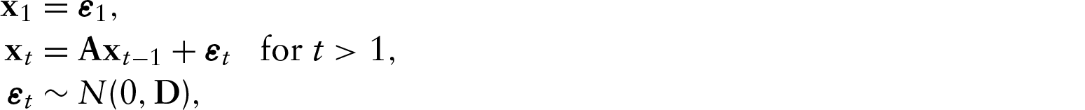
To build a model for equilibrium data, first consider a first-order vector autoregres- sive, or VAR(1) model for time-series data for a system with p genes with no correlation in the error term between genes (Lütkepohl, 2005). We can write the model as
Autoregressive models have been broadly used to infer gene networks from time-series data, with approaches ranging from penalized regression (LASSO, elastic net) to Bayesian model averaging (BMA) to dynamic Bayesian networks (DBN). Michailidis and dAlché Buc (2013) review many of these approaches to modelling time series using autoregressive models.
At first glance, the VAR(1) model does not appear to be applicable to steady-state data. However, if the eigenvalues of
Equilibrium distribution
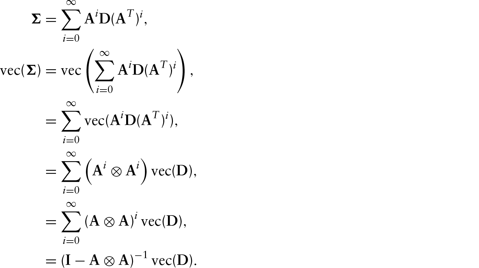
Since this is a Gaussian VAR model, we can write the equilibrium distribution as

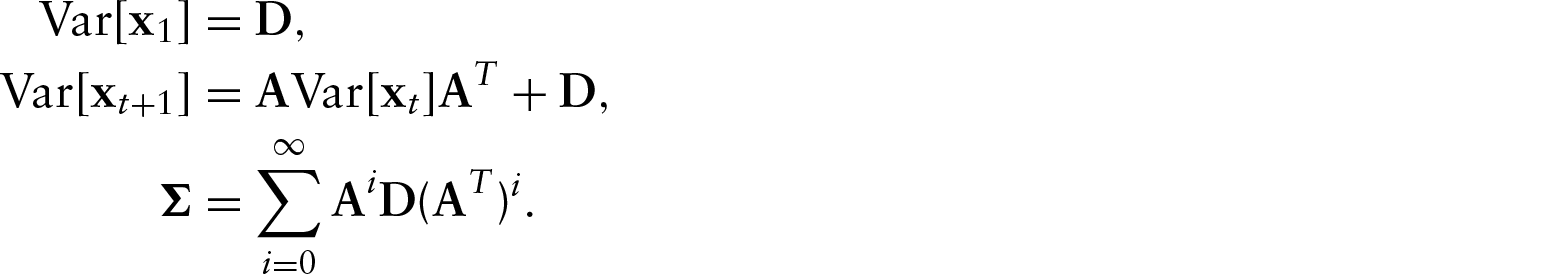
We will call this the summation identity (Sheppard, 2013).
Another expression for the asymptotic variance uses the identity

When looking at steady-state data as opposed to time-series data, we must rely on the relationship between

We can state the identifiability problem as follows. Under what conditions is the map

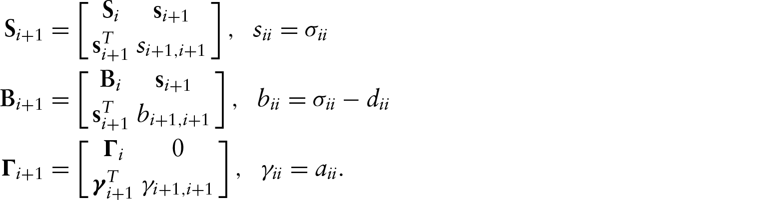
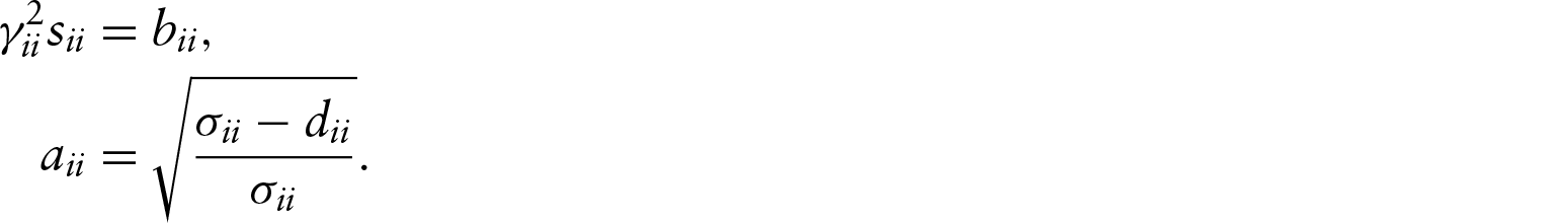
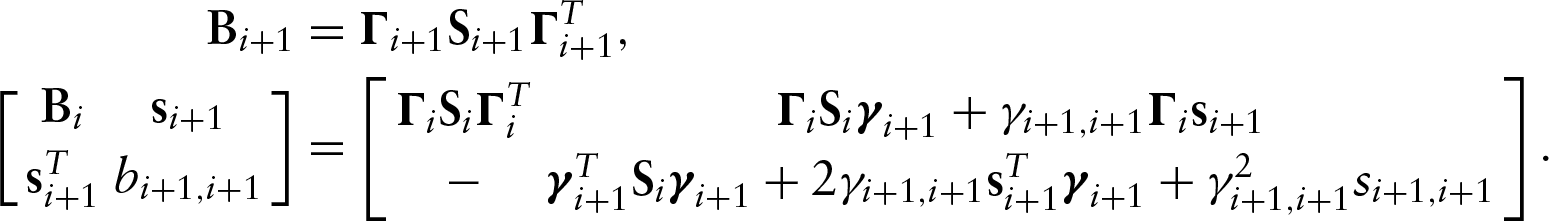
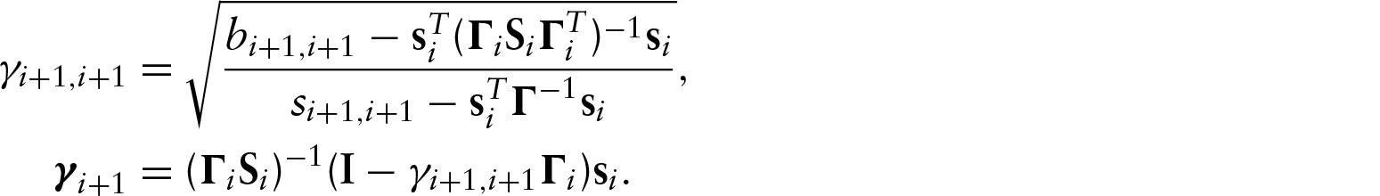
Parameter counting yields a necessary condition, but it is not a sufficient condition. We have not found sufficient conditions in the most general case. We have, however, been able to examine identifiability in two specific examples, one acyclic and one cyclic. To assess the identifiability of a specific model, we used the recursive identity,

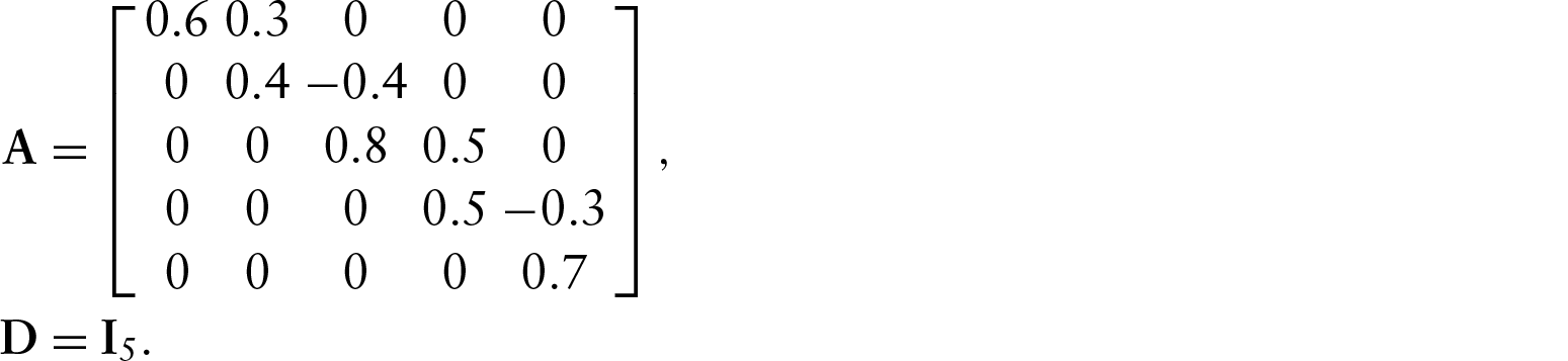
The first example is a five-dimensional model with a simple network structure, given in Figure 1. This model has four off-diagonal non-zero elements in
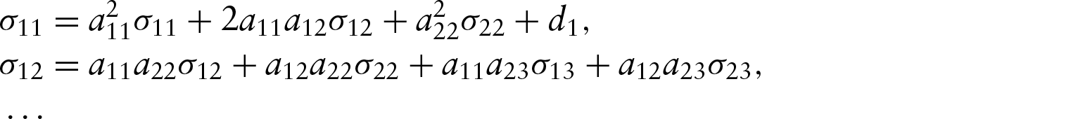
where
To test the parameter solutions, we used the following model parameters:
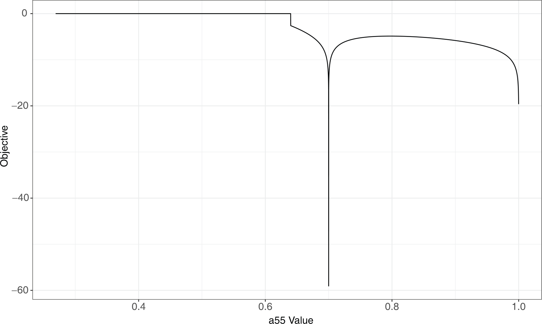
The grid search was performed by allowing
The network structure for the cyclic identifiability example
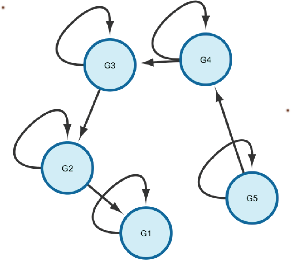
The network structure for the cyclic identifiability example
Grid search for solutions of the acyclic identifiability example. The objective function is minimized at the true value of
, showing that the model is identifiable in this example
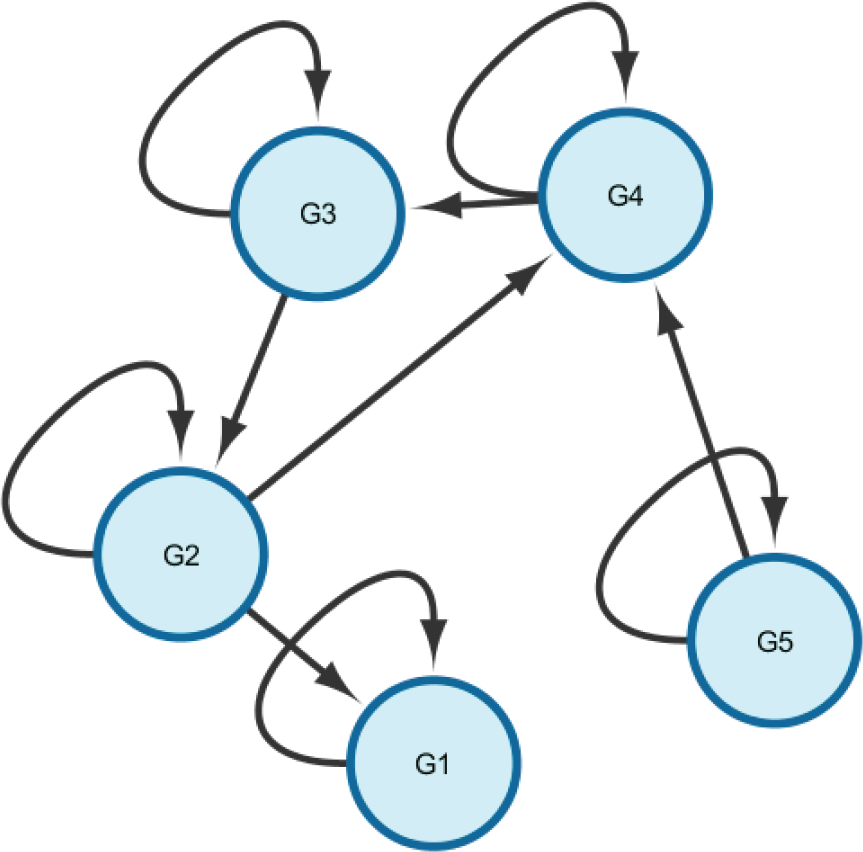
Our second example involves a cyclic network. We added a single edge to the previous network, making a 3-node cycle, as shown in Figure 3. We used the following model parameters:
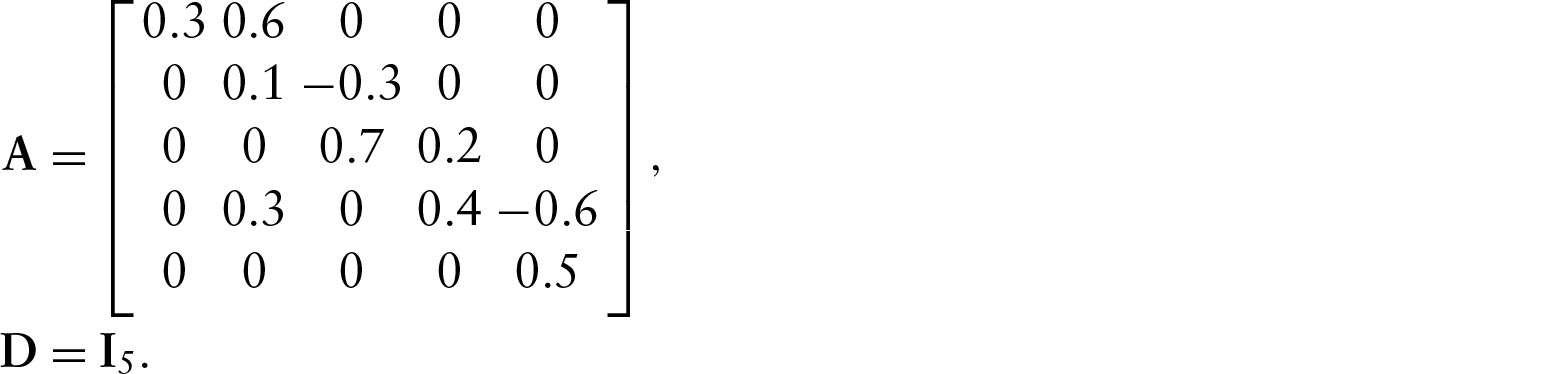
The network structure for the cyclic identifiability example
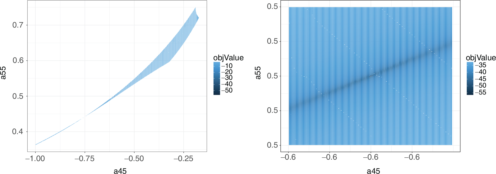
Grid search for solutions of the cyclic identifiability example showing the value of the objective function at each point searched. The left plot shows the grid search over the entire model space, while the right plot is zoomed in on the true parameter value. The white areas indicate parameter values that result in invalid solutions. The true solution at (
0.6, 0.5) is the only valid solution
Although the parameter counting condition is helpful and results in identifiability in at least a couple of examples, it is important to find a more general result for identifiability.
We now find a more general condition for identifiablity within a specific subset of VAR(1) models. We do this by restricting the model considerably to make the analysis more tractable. First, we constrain
Consider the model as constrained earlier. We order the nodes in the network topologically, meaning that there are no edges from node


Now, for
This gives us
We solve for
Notice here that the expression for

where


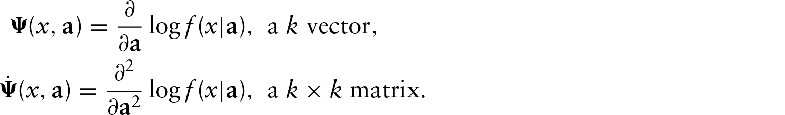
The appendix contains derivations of the first- and second-partial derivatives and show that they exist and are continuous. For example, the first partial derivatives take the form

Now let

where the

where
These results, along with the earlier proof of identifiability and the form of the constraints on
In addition to asymptotic consistency and efficiency, we also can form a likelihood-ratio test for the existence of an edge.

has a
We have an asymptotic distribution for the MLE, and now we assess the quality of its approximation in finite samples via simulation. Because of the complexity of the calculations involved in finding the Fisher information matrix, we will restrict ourselves to a two-dimensional model. This model has three parameters for

so

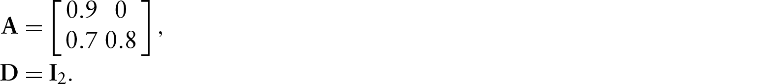
Using these values, the asymptotic variance of the MLE for

To test this, we performed a simulation where we generated
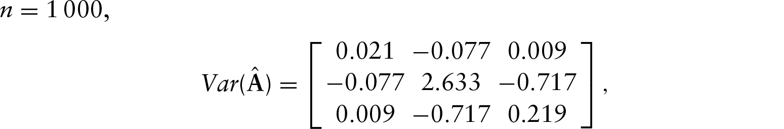
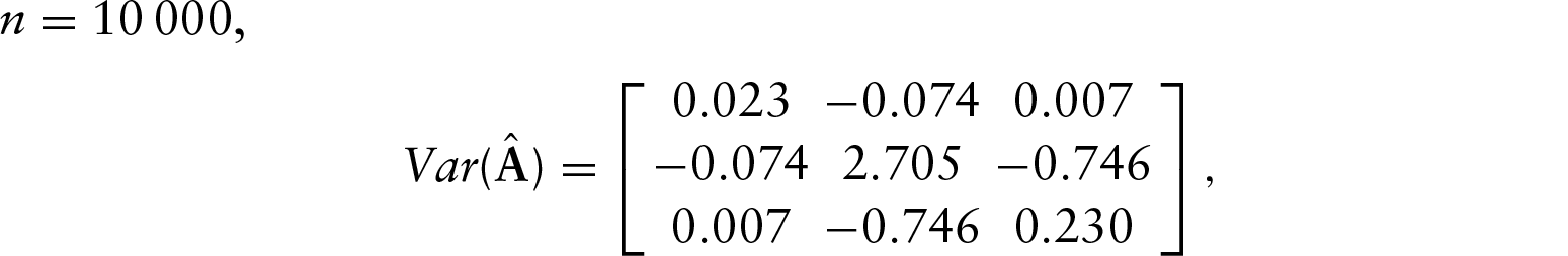
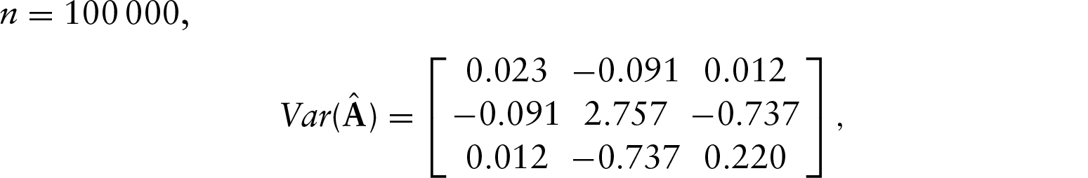
These results show that the asymptotic variance approximates the finite sample variances quite well, and so provide support for the asymptotic theory.
Simulation results: Coverage
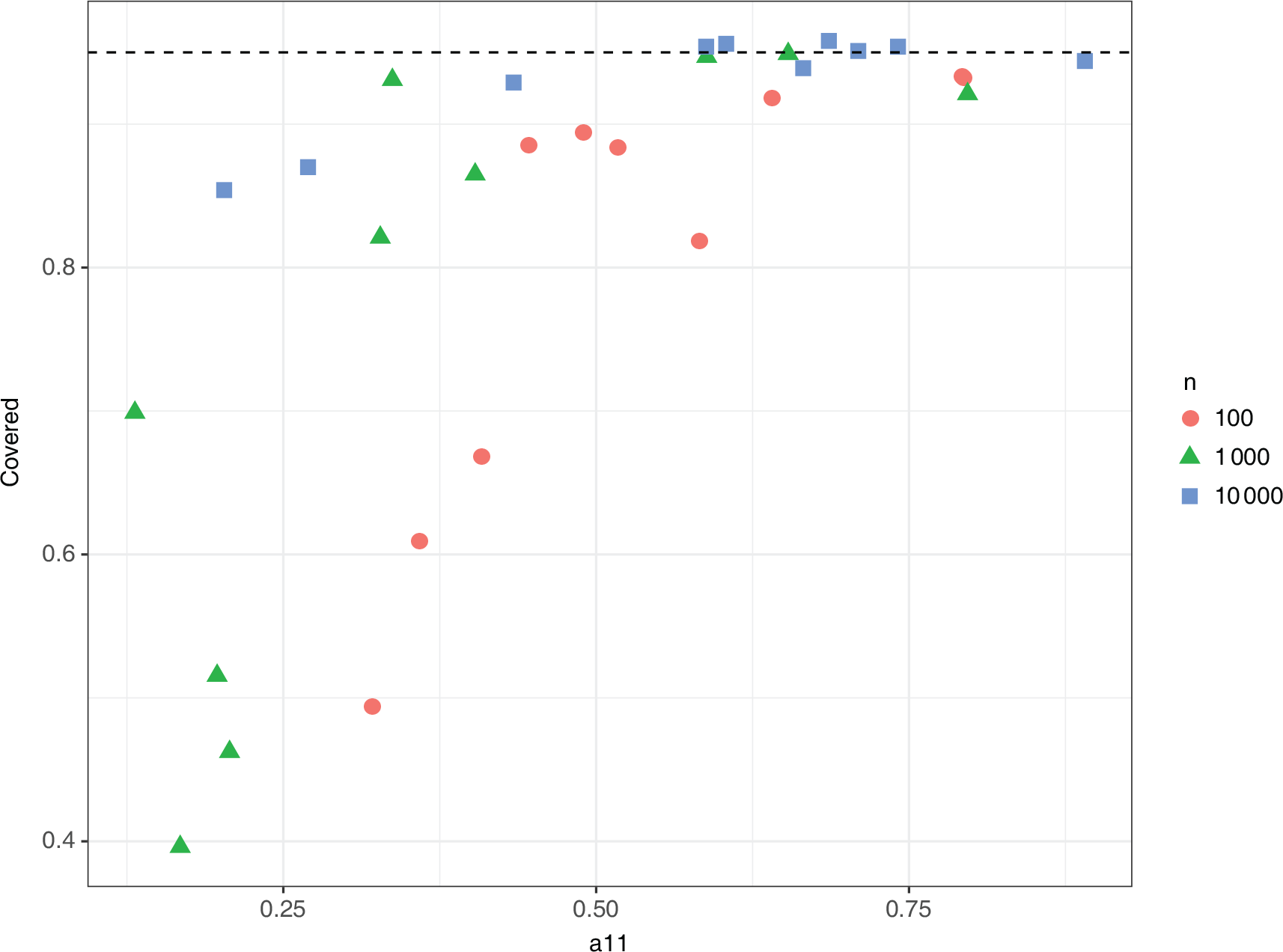
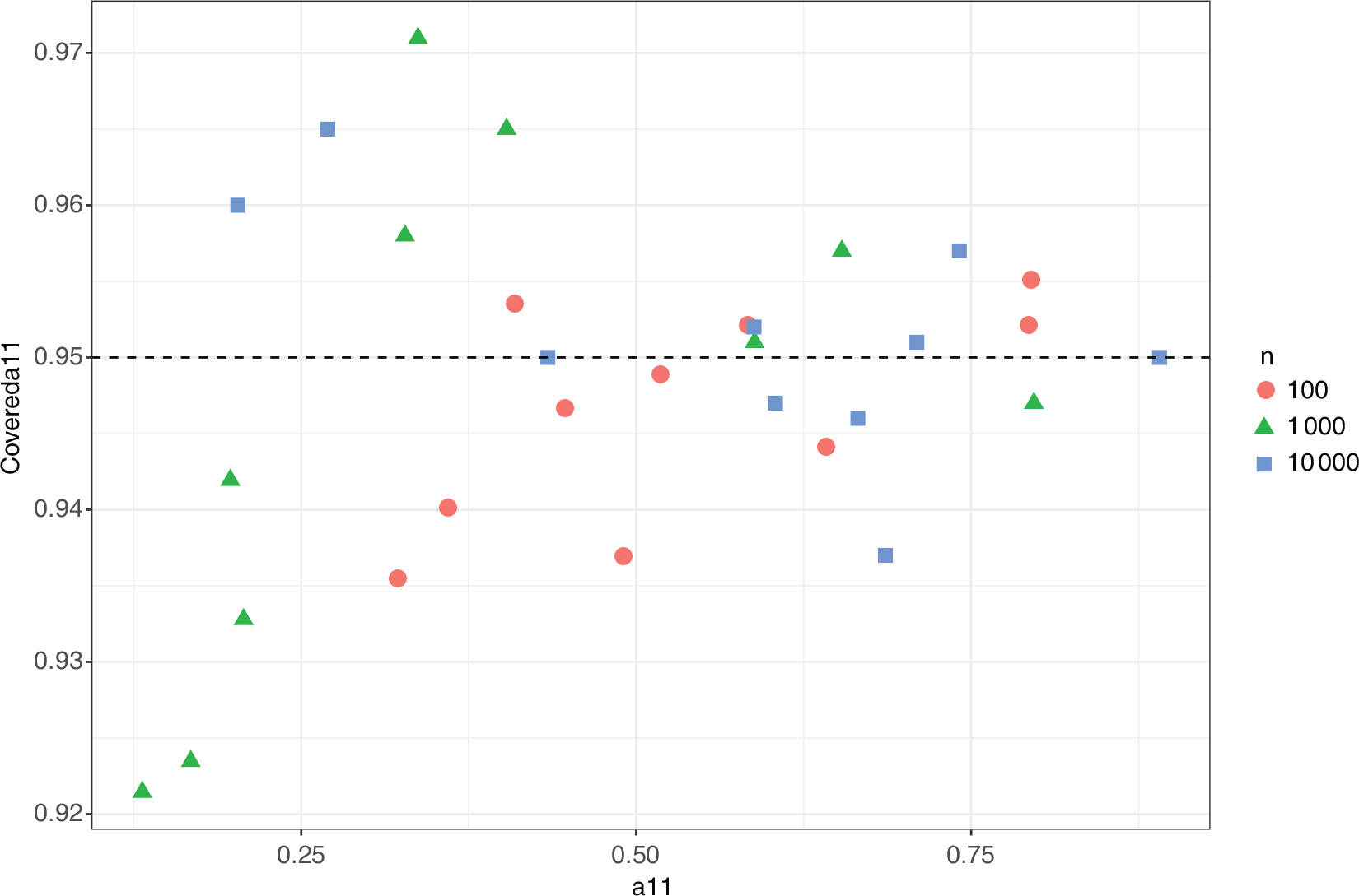
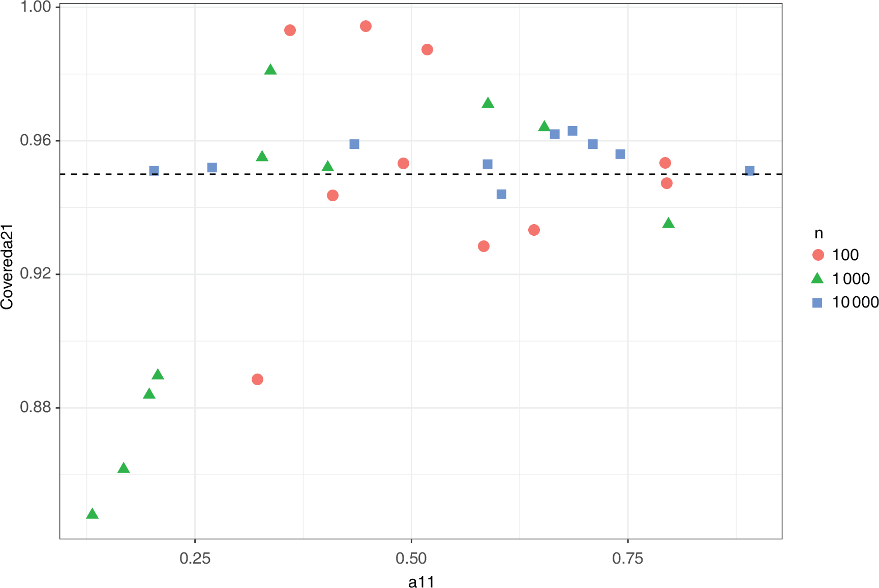
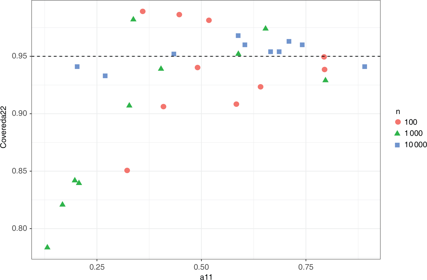
Another way to assess the accuracy of the asymptotic approximation for finite samples is to look at the coverage of the resulting confidence intervals. To do this, we used the same two-dimensional model as earlier. In each single simulation,
We carried out this procedure 10 times each for
We note that with small
Joint coverage for
using the asymptotic distribution of the MLE]Joint coverage for all parameters of
using the 95% confidence interval from the multivariate normal asymptotic distribution of the MLE
Joint coverage for
using the asymptotic distribution of the MLE]Joint coverage for all parameters of
using the 95% confidence interval from the multivariate normal asymptotic distribution of the MLE
Marginal coverage for
using the asymptotic distribution of the MLE]Marginal coverage for
using the 95% confidence interval from the asymptotic distribution of the MLE
Marginal coverage for
using the asymptotic distribution of the MLE]Marginal coverage for
using the 95% confidence interval from the asymptotic distribution of the MLE
Marginal coverage for
using the asymptotic distribution of the MLE]Marginal coverage for
using the 95% confidence interval from the asymptotic distribution of the MLE
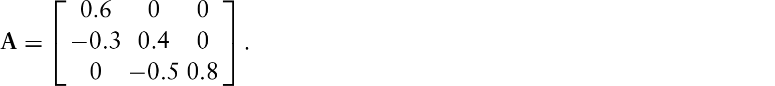
We now assess the validity of the likelihood-ratio test for the simple VAR equilibrium model. To test this, we used a three-dimensional system with
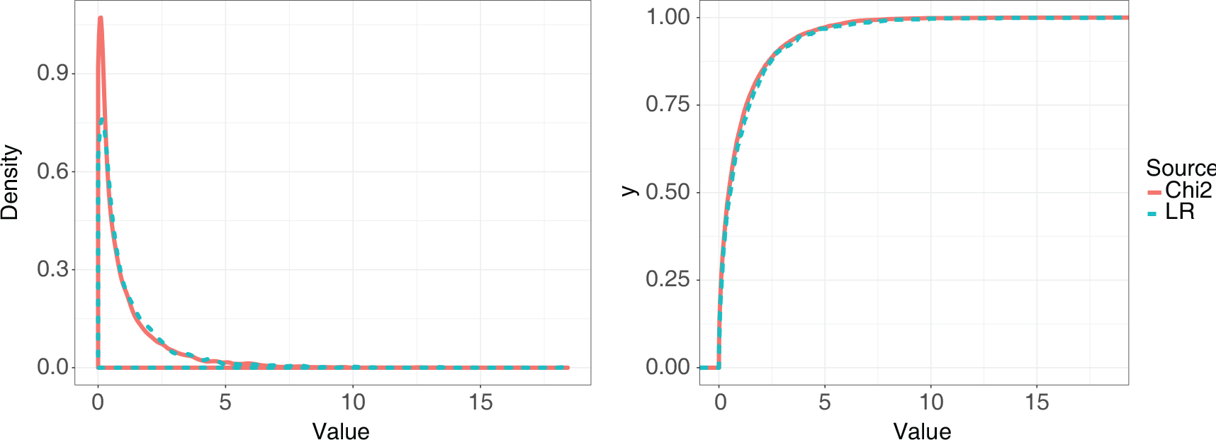
To obtain the empirical distribution of the test statistic, we generated 10 000 samples from the equilibrium distribution and calculated the likelihood ratio for those data. We repeated this 1 000 times to get a distribution values of the statistic. Figure 9 shows the distribution compared with a
Comparison of the empirical distribution of the likelihood ratio statistic to test for an additional edge in the VAR equilibrium problem with a
distribution with one degree of freedom. The left-hand plot shows the density of the test statistic compared with the
distribution, while the right-hand plot shows the empirical CDF comparison
We have shown by simulation that the asymptotic distributions of estimators and likelihood-ratio test statistics provide good approximations to finite-sample distributions in several example scenarios. What happens when we try to apply the method in situations where the model is not known to be correct? The matrix
GeneNetWeaver data
To look at the method in a more realistic setting, we need a reasonable size network where the truth is known. For this we used networks from the DREAM4 in silico network challenge competition (http://dreamchallenges.org/project/dream4-in-[silico-network-challenge/]). The 10-gene networks from the competition are a good size for analysis, include cycles, and are known. The original data used in the competition include time-series data simulating a perturbation to the network. The first and last time points do correspond to a stable equilibrium for the network, but these cannot be used for our purposes because the original data do not include enough separate time series from which to get samples.
However, the software used to generate the data, GeneNetWeaver, is available online at http://gnw.sourceforge.net/(Marbach et al., 2009; Schaffter et al., 2011). The software can be configured to generate any number of independent time series from a given network model. The data are generated according to a dynamical model using ordinary differential equations with added stochastic noise. For the time-series data, the network begins at equilibrium, and then the network is artificially perturbed for the first half of the time course. At the midpoint of the time course, the perturbation is removed and the network is allowed to return to its equilibrium state by the end of the time course. The GeneNetWeaver software is designed to provide a rich simulation of the dynamics of biological regulatory networks. The ODEs used include terms simulating transcription and translation rates as well as protein degradation rates, and simulates mRNA levels and protein levels simultaneously. Noise is added to the system to simulate both random fluctuations in the actual levels of mRNA and protein as well as measurement error.
We used GeneNetWeaver to generate time-series data using the network model used in the first 10-gene network from the DREAM4 competition. The GeneNetWeaver software has this network available as a pre-configured model from which data can be generated. The network has 10 nodes and 15 non-self edges, including a cycle involving 3 genes. All settings for data generation were the same as those used in the DREAM4 competition, including the amount of added noise to the system and the model of noise in microarrays. We used GeneNetWeaver to generate 100 random time series of 21 points each from the model and took the first and last time points as samples from the equilibrium distribution.
Method application
To see how the VAR equilibrium method works on these data, we used the known network structure as our initial model for
To find the MLE for the model, we randomly initialized
After
This gave an estimate of the parameters for the true model, but in order to test individual edges, we needed to find the MLE for models adjacent to the true model. These models are defined by taking the original network structure and adding or removing a single edge. When removing edges, we needed to ensure that the connectivity of the graph was not broken. Three of the edges in the original network, if removed, would isolate a single node. This leaves 12 of the original 15 edges available to be tested. Adding an edge does not create problems, and thus we were able to test all 75 extra edges. With the results from the true model and the 87 testable models, we could see which edges the likelihood ratio test identified as significant.
Running the above optimization scheme for each of the 88 models resulted in an approximate MLE for each model. Because these optimizations were run independently for each model and the model space is not necessarily fully searched, this resulted in some mis-ordering of the models. That is, the MLE found for one model resulted in a likelihood that was worse than that of a model in which some of the parameters of the first model are constrained to be zero. This is never allowed since the parameters of the smaller model can be used for the larger model, resulting in the same likelihood.
To fix the ordering issue, we performed a second optimization step for each target model. We initialized
Results
We applied the optimization scheme described earlier to both the initial and final time point data from the generated data from GeneNetWeaver. For each model explored, we obtained the best log-likelihood value for comparison. We then compared the true model with each other model, either with one less or one more edge, and computed the likelihood ratio statistic for testing the edge. From the likelihood ratio statistic we computed a p-value by comparing the value to a
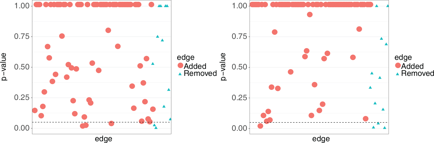
Ideally, the p-values corresponding to the 12 edges which are in the true network would be low and the p-values for the 75 edges added to the true model would be high. Figure 10 shows the results for both the first and the last time point. Looking at the circles, we find that 7 of the 150 edges added to the true network were identified as true edges at
p-values for testing edges in GeneNetWeaver data]p-values for each tested edge in the GeneNetWeaver data. Circles correspond to edges added to the true network (false edges) and triangles correspond to edges removed from the true network (true edges). The left figure is using data from the first time point and the right figure is using data from the last time point. The dashed line corresponds with a
-value of 0.05
Steady-state gene expression data present a challenge in inferring directional edges. We have presented a model which can be used to test for the existence of edges in such data. We have derived asymptotic properties of estimators and tests for this model in a constrained, but still reasonably large subset of the possible models, and we found that the resulting asymptotic approximations performed well in some finite-sample settings. The derivation of necessary and sufficient conditions for identifiability in the fully general case is a topic for future research.
The identifiability problem is also found in structural equation modeling (SEM) (Bentler and Weeks, 1980). SEM is similar to a VAR model in that it specifies relationships among a set of variables. SEM, however, relates the variables without considering the time element. If

We have shown that even in cases where the theory has not been validated, the VAR equilibrium method can still identify true relationships among genes. This is evident in the analysis of the GeneNetWeaver data, where true edges were identified more consistently than extraneous edges.
If the network is partially known, then the likelihood ratio statistic can be used to test for extra edges and thus build up a more comprehensive view of the network. As an example, we may want to learn about a network perturbed with a certain drug. If the unperturbed network is known, we can test edges in and around that network using the perturbation data to learn about the changes induced by the drug. Since we may not expect the entire network to change, the VAR equilibrium method takes advantage of prior knowledge about the network structure.
To apply the VAR equilibrium-based likelihood ratio test method to steady-state data without a known network to start from will take further development. One way to go about this would be to take a subset of genes and look at all possible network structures for those genes. For each model, the steady-state data would be used to maximize the likelihood. One could then combine the models using a BMA approach. To do this, the integrated likelihood needs to be approximated for each model. As a starting point, the Bayesian Information Criteria (BIC) could be used. The BIC is equal to
Declaration of Conflicting Interests
The author(s) declared no potential conflicts of interest with respect to the research,authorship and/or publication of this article.
Funding
This research was supported by NIH grants U54-HL127624, R01-HD054511 and R01-HD070936. Raftery's research was also partly supported by the Center for Advanced Study in the Behavioral Sciences at Stanford University.