Sage Journals: Discover world-class research

Abstract

Currently there is little guidance on the power considerations for the multiple-group (controlled) interrupted time series design (MG-ITSA). In this study, simulations estimated power based on the number of time periods, the number of control units, when the treatment is introduced, and the degree of autocorrelation. The measures of effect were the difference in differences (DID) in level and the DID in trend. Power was evaluated at three different effect sizes. Higher power was generally associated with longer studies, more control units, larger effect sizes, and decreasing autocorrelation. Introducing the treatment at the halfway point in the study typically produced higher power than elsewhere for DID in trend. DID in level required fewer time periods to achieve the desired power than the DID in trend. The results show that to increase power, a researcher can increase the number of control units, increase the number of time periods, utilize the DID in level as the measure of effect, and maximize the effect size. Autocorrelation cannot be readily manipulated, and therefore must be accounted for in the time series regression model. Health researchers must consider the many factors highlighted here that uniquely affect power when determining the most efficient way to conduct an MG-ITSA study.

Keywords

interrupted time series analysis multiple-group interrupted time series analysis controlled interrupted time series analysis power sample size autocorrelation

Introduction

Interrupted Time Series Analysis (ITSA) is a widely used research design in healthcare for evaluating the impact of treatments, policy changes, and natural events. In this approach, the outcome of interest is measured as a time series—repeated observations taken at regular intervals—typically at an aggregate level (e.g., morbidity or mortality rates, average costs). A single unit, such as a hospital, city, or region, is exposed to a specific “treatment,” which is expected to cause a noticeable change, or “interruption,” in the level and/or trend of the time series following its introduction (Campbell & Stanley, 1966; Shadish et al., 2002). ITSA is generally considered to have strong internal validity, largely because it helps control for regression to the mean (Campbell & Stanley, 1966; Linden, 2013; Shadish et al., 2002). It also tends to demonstrate good external validity, particularly when applied at the population level or when findings can be generalized across different units, treatments, or contexts (Campbell & Stanley, 1966; Shadish et al., 2002).

Despite its strengths, the single-group version of ITSA (SG-ITSA) has notable limitations. Some major threats to the internal validity of a SG-ITSA include history (external events coinciding with the intervention), maturation (natural changes in participants over time), instrumentation (changes in how the outcome is measured) and attrition (participants leaving the study) (Campbell & Stanley, 1966; Shadish et al., 2002). These factors can provide alternative explanations for observed effects, potentially confounding the interpretation of the intervention’s true impact. Recent studies have further shown that the SG-ITSA design may overlook the influence of external factors on the time series, leading to erroneous causal conclusions, or it may produce misleading interpretations when a correct directional change in the outcome occurs before the treatment is implemented (Linden, 2017a; Linden & Yarnold, 2016). These problems can persist even in more complex designs that involve multiple transitions between treatment and non-treatment periods (Linden, 2017b).

The limitations of the SG-ITSA can be overcome with the inclusion of one or more control units that are comparable to the treated unit on both the baseline level and trend of the outcome variable (Linden, 2015; 2017a; 2017b) as well as on other observed pretreatment characteristics (Abadie et al., 2010; Linden, 2018). This ITSA design is generally referred to as a multiple-group ITSA or controlled ITSA (from here on out in the paper, it will be referred to as MG-ITSA). Only control units that are comparable to the treated unit in all observable ways can offer a plausible counterfactual when estimating treatment effects (Rubin, 1974).

Despite the ubiquity of healthcare studies using the MG-ITSA design (for some recent examples, see Ansermino et al., 2025; Aye et al., 2024; Barbalat et al., 2025; Du et al., 2025; Gressler et al., 2025; Luo et al., 2025; Tsunemitsu et al., 2025; Walter et al., 2025; Wanigaratne et al., 2025; Wyper et al., 2023), very few studies conduct a power analysis. This is mainly due to the fact that most MG-ITSA studies are retrospective, making formal power analyses both conceptually inappropriate and potentially misleading (Dziak et al., 2021). In a sampling of three studies in which the MG-ITSA design was applied prospectively, three different approaches were used to estimate power. Fanshawe et al. (2022) estimated power in their MG-ITSA study by first fitting autoregressive integrated moving average (ARIMA) models to each site’s pre-intervention time series, capturing trends and autocorrelation. They then simulated post-intervention outcomes under specified effect sizes for the treated sites and combined these with the control site forecasts to generate counterfactuals. Yelland et al. (2015) appears to have used cluster-level standard deviations and intra-class correlation to estimate power to detect a relative change in the outcome, but the exact approach was not clearly defined. Power et al. (2014) used a simple baseline average versus end of study average comparison to compute power. They suggested that this was preferable to basing the power calculation on an interrupted time series using a fixed number of cases per month, because they did not know in advance how the sites would choose to implement their activities or the likely impact of these activities. These findings highlight the inconsistency in how power analyses for the MG-ITSA design are currently being conducted and the need for formal tools specific to MG-ITSA. That said, Schochet (2022) developed closed-form expressions that quantify the statistical power and minimum detectable effect size of an MG-ITSA estimator given the design’s sample size, timing structure, and autocorrelation. In Schochet’s framework, study units are treated as clusters for variance estimation. An important consideration when using this approach is that it implicitly requires at least two clusters for identification, and many more for reliable cluster-robust inference. Thus, it may not be suitable for the most common MG-ITSA scenario in which there is a single treated unit, there may be few comparable controls available, and all units are pure individual units rather than representing clusters.

This paper adds to the limited literature on power for the MG-ITSA study by conducting a comprehensive set of simulations to address factors unique to the study design when estimating sample size/power using time series regression. These factors include the total number of time periods under study, the number of control units serving as comparators, the time point within the overall time series when the treatment is introduced, handling of the autocorrelated nature of the data (i.e., the degree to which errors between consecutive observations are serially correlated), and the measure of effect which can be expressed as either differences in the pre-to post-treatment change in level (i.e. difference in differences in level) or differences in the pre-to post-treatment change in trend (i.e. difference in differences in trend) of the outcome variable. In contrast to Schochet (2022), here a single treatment unit is examined and compared to controls which are treated as individual units and not clusters.

We examine the difference in differences in level and trend of the time series using ordinary least squares (OLS) regression adjusted with Newey-West standard errors (Newey & West, 1987). Simulations are repeated for the number of time periods ranging from 10 to 50, the number of control units ranging from 4 to 20, autocorrelation ranging from −0.90 to 0.90, and when the introduction of the treatment occurs at one-third, one-half, and two-thirds of the length of the time series. Additionally, a worked example is presented to demonstrate how the simulation approach described in the paper can be used to estimate the number time periods necessary using specific input criteria to achieve the desired power in a prospective healthcare study. The generalized results of these analyses, as well as a new community-contributed package for Stata called POWER_ITSA (Linden, 2025b) will guide healthcare researchers in determining the most efficient way to achieve anticipated treatment effects when using the MG-ITSA design.

Methods

The MG-ITSA regression model assumes the following form (Linden, 2015, 2017c):

Y_{t} = β_{0} + β_{1} T_{t} + β_{2} X_{t} + β_{3} X_{t} T_{t} + β_{4} Z + β_{5} Z T_{t} + β_{6} Z X_{t} + β_{7} Z X_{t} T_{t} + ϵ_{t}

(1)

where Y_t is the aggregated outcome variable measured at each time-point t, T_t is the time since the start of the study; X_t is a dummy variable representing the treatment (pre-treatment periods = 0, otherwise 1); Z is a dummy variable to denote the cohort assignment (treatment or control); and X_tT_t, ZT_t, ZX_t and ZX_tT_t are all interaction terms among these variables. Coefficients β₀ – β₃ represent the control group and the coefficients β₄ – β₇ represent values of the treatment unit. More specifically, β₀ represents the intercept, or starting level of the aggregated outcome variable of the control group; β₁ is the slope, or trajectory of the outcome variable for the control group until the introduction of the treatment; β₂ represents the intercept at the time-point immediately following the introduction of the treatment and indicates whether there was a change in the level of the outcome immediately following the introduction of the treatment for the control group; β₃ represents the change in slope or trajectory of the outcome in the control group after introduction of the treatment until the end of the study; β₄ represents the difference in the level (intercept) of the outcome variable between the treatment unit and controls prior to the treatment; β₅ represents the difference in the trajectory (slope) of the outcome variable between the treatment unit and controls prior to the treatment; β₆ indicates the difference between the treatment unit and controls in the predicted level of the outcome variable versus their counterfactuals in the period immediately following introduction of the treatment (i.e. difference in differences in level), and β₇ represents the difference between the treatment unit and controls in the slope (trend) of the outcome variable after initiation of the treatment compared with pre-treatment (i.e. difference in differences in trend) (Linden, 2015). When the random error terms follow a first-order autoregressive (AR1) process,

ϵ_{t} = {ρ ϵ}_{t - 1} + u_{t}

(2)

where, the autocorrelation parameter ρ is the correlation coefficient between adjacent error terms, such that |ρ| < 1, and the disturbances u_t are independent N (0,σ²) (see Kutner et al. (2005) for a detailed discussion of autocorrelation in time-series regression models).

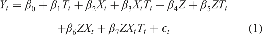
The two parameters (β₄ and β₅) play a particularly important role in establishing whether the treatment unit and controls are balanced on both the level and trend of the outcome variable in the pre-treatment period. If these data are from an RCT, we would expect similar levels and trends prior to the treatment. However, in an observational study where equivalence between groups cannot be ensured, any observed differences will likely raise concerns about the ability to draw causal inferences about the outcomes (Linden, 2015, 2017c). For a visual depiction of these parameters the reader is referred to Linden (2015, 2022).

The POWER_ITSA Package for Stata

All simulations in the current study were conducted using the new community-contributed package for Stata called POWER_ITSA (Linden, 2025b). The sub-routine called POWER_MULTI_ITSA takes values representing coefficients from the MG-ITSA regression model (Equation (1)) to generate artificial datasets containing one treated unit and a user-specified number of control units. POWER_MULTI_ITSA takes additional inputs pertaining to the overall simulation process itself.

In the current study, the following options were specified as inputs for POWER_MULTI_ITSA:

The number of time periods in the series (ranging from 10 to 50). The minimum of 10 periods was based on the results of Zhang et al. (2011) and Linden (2025a) that showed inconsistent power estimates for time series with less than 10 periods in simulation studies of power for the SG-ITSA design. The upper limit of 50 time periods represents a reasonably long time series for most ITSA studies.

The time period when the treatment begins (set at one-third, one-half, and two-thirds of the length of the time series). These treatment initiation times are consistent with those used in simulation studies of power for the SG-ITSA design (Hawley et al., 2019; Linden, 2025a; Zhang et al., 2011).

The number of controls (set to range from 4 to 20 in increments of 4, except when evaluating autocorrelation where the number of controls was set to 12). This is a reasonably large range of controls that might be available in most health care settings (e.g. medical groups, wards, hospitals, laboratories, etc.).

The starting level (intercept) of the control time series (set to 10). This is consistent with (Linden, 2025a). A non-zero intercept ensures ensure that simulated datasets will not produce negative values.

The starting level of the treatment unit’s time series (set to 10). This is consistent with (Linden, 2025a). A non-zero intercept ensures ensure that simulated datasets will not produce negative values.

The trend (slope) of the controls’ time series prior to the treatment (set to 1). This small period over period increase is intended to represent a small underlying secular trend in the time series.

The trend (slope) of the treatment unit’s time series prior to the treatment (set to 1). This small period over period increase is intended to represent a small underlying secular trend in the time series.

The change in the level of the controls’ time series immediately following the introduction of the treatment versus the counterfactual at that time-point (set to 0). We do not expect any factor to influence the level of the controls’ time series.

The change in the level of the treatment unit’s time series immediately following the introduction of the treatment versus the counterfactual at that time-point (set to increase in increments of 2, 2.5, and 3 points when evaluating change in level, else 0). These values represent a 20%, 25% and 30% immediate increase in level versus the counterfactual at the first post-treatment time point and are consistent with the range of effect sizes reported in (Linden, 2025a) for time periods 10 through 50 with 80% power and alpha 0.05. Additionally, power curves were computed for 5 points (50%) to allow for a direct comparison between level and trend at 25% and 50%.

The trend (slope) of the controls’ time series after introduction of the treatment (set to 1). In the absence of a treatment, we expect the controls’ time series to continue unchanged from baseline (set to 1 to represent a small continued secular trend from baseline).

The trend (slope) of the treatment unit’s time series after introduction of the treatment (set to increase in increments of 1.25, 1.5, and 2 points when evaluating change in trend, else 0). These values represent a 25%, 50% and 100% increase in the post-treatment trend and are consistent with the range of effect sizes reported in (Linden, 2025a) for time periods 10 through 50 with 80% power and alpha 0.05.

The correlation coefficient between adjacent (autoregressive) error terms (ranging from −0.9 to 0.9, in increments of 0.3 for both treated unit and control units for specific analyses of autocorrelation, otherwise the autocorrelation was set to 0.2 for both treated and control units), representing a small positive autocorrelation. This is consistent with that used in Linden (2025a).

1 standard deviation (SD) was used in generating the normally distributed random error term for the treatment unit and 2 SDs for controls. The 1 SD random error for the treatment unit is consistent with that used in Linden (2025a). The slightly higher level of random error used for generating the control groups’ time series is intended to represent the typical scenario where matched controls may have a similar mean baseline level or trend to that of the treatment unit, but likely differ in their variability than the control unit (Linden, 2018).

Sensitivity analyses were performed to determine if differing baseline levels and trends between treatment and control units impact power curves. For level change, the starting value of the treatment unit’s time series was 10 and the starting value of the treatment unit’s time series was 8. For trend change, the baseline trend for the treated unit was 5 and the baseline trend for the control units was 1. These values were chosen because, in practice, controls are matched to treated units based on comparability of baseline level and trend to the treated unit (Linden, 2018). Therefore, small differences may be expected when the pool of controls is small. All other inputs remained unchanged from above.

The percentage bias of the β₆ and β₇ coefficients (difference in differences in level and difference in differences in trend, respectively) was calculated for the base scenario in which the treatment was introduced at the halfway point in the time series, the number of controls ranged from 4 to 20, the number of time periods ranged from 10 to 50, and autocorrelation was set to 0.20 for both treatment and control units. Additionally, percentage bias was computed for values of autocorrelation ranging from −0.9 to 0.9, in increments of 0.3, where the number of controls was set to 12 and all other input values were set as in the base scenarios for difference in differences in level and trend. Percentage bias is computed as $(\frac{\bar{\hat{β}} - β}{β})$ x 100, where $\bar{\hat{β}}$ is the mean estimate across all simulations and $β$ is the true value for the estimate of interest (Burton et al., 2006).

Figure 1 visually summarizes the data generating process (DGP) for evaluating differences in change in trend and level, respectively. As shown, the treatment unit and controls are comparable on the baseline level and trend. However, while the controls’ time series do not change after introduction of the treatment, the treatment unit’s time series increases incrementally by 1.25, 1.50, and 2 absolute points for a trend change (representing a 25%, 50% and 100% increase) and by 2, 2.5, and 3 absolute points for a level change versus the counterfactual (representing a 20%, 25% and 30% increase).

Figure 1

A Visual Depiction of the Data Generating Process to Detect an (A) Difference Between the Treated Unit and Controls’ Change in the Post-treatment Trend From the Pre-treatment Trend (Representing a 25%, 50% and 100% Increase in the Treatment Unit’s Trend), and (B) the Difference Between the Treated Unit and Controls’ Post-Treatment Level From Their Respective Counterfactuals (Representing a 20%, 25% and 30% Step Increase in the Treatment Unit’s Level Versus the Counterfactual)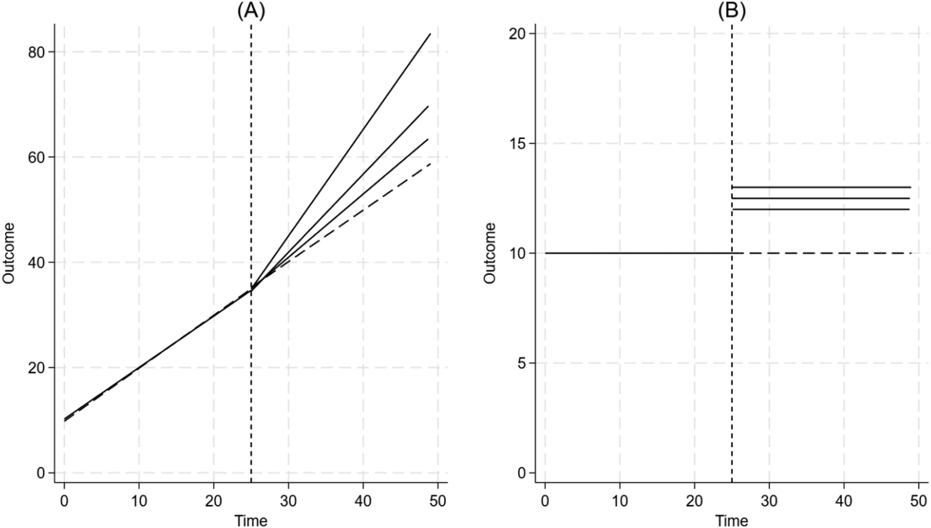

For each time series dataset generated (containing the treatment unit and the number of control units specified), POWER_MULTI_ITSA estimates the treatment effects represented by coefficients β₆ and β₇ in equation (1) (i.e. the difference in differences in level of the time series and difference in differences in trend, respectively). This study used the default estimation model which is a generalized linear model (GLM) adjusting for autocorrelation with Newey-West standard errors (Newey & West, 1987) for a lag (1) autocorrelation structure. After model estimation, a Wald test was utilized to determine if the coefficient β₆ or β₇ is 0 (representing the difference in differences in level and difference in differences in trend, respectively), and the associated P-value was saved. For all scenarios (i.e. varying numbers of time periods, varying number of control units, varying levels of autocorrelation, varying effect sizes, and varying the time-point of introduction of the treatment within the time-series) 2,000 simulated datasets were generated and power was computed as the proportion of simulations in which p < 0.05 (see Landau & Stahl [2013] for a comprehensive tutorial on designing simulation studies for estimating power). The number of simulations was selected after examining a set of preliminary results across a range of 100 to 10,000 simulations. It was found that the results generally stabilized at 1000 simulations, meaning they were comparable to those from 10,000 simulations. Ultimately, 2000 simulations were chosen as a compromise between resource demands and enhanced accuracy. Stata^TM version 19.0 was used for conducting all analyses.

The study design presented in this paper aims to identify generalizable patterns in the factors that influence power within a multi-group interrupted time series analysis, such as the number of time periods, the number of control groups, the level of autocorrelation, etc. As such, the current study design excludes special cases such as higher-order autocorrelation, seasonal dynamics, unusual events and other non-linear features.

Results

Difference in Differences in Trend

Figure 2 illustrates that power consistently increases as a function of an increasing number of control units, an increasing number of time periods, and increasing effect size when the treatment is introduced at the halfway point in the time series. As shown, with a 25% effect size, it takes over 30 periods for any sized control group to achieve approximately 80% power. Conversely, with a large effect size (100%), all control units can achieve over 80% power within 20 time periods.

Figure 2

The Impact of the Number of Control Units and the Number of Time Periods on Power for a Difference in Differences in Trend, when the Treatment Begins at the Halfway Point in the Time Series. Panel A Represents a 25% Effect, Panel B Represents a 50% Effect, and Panel C Represents a 100% Effect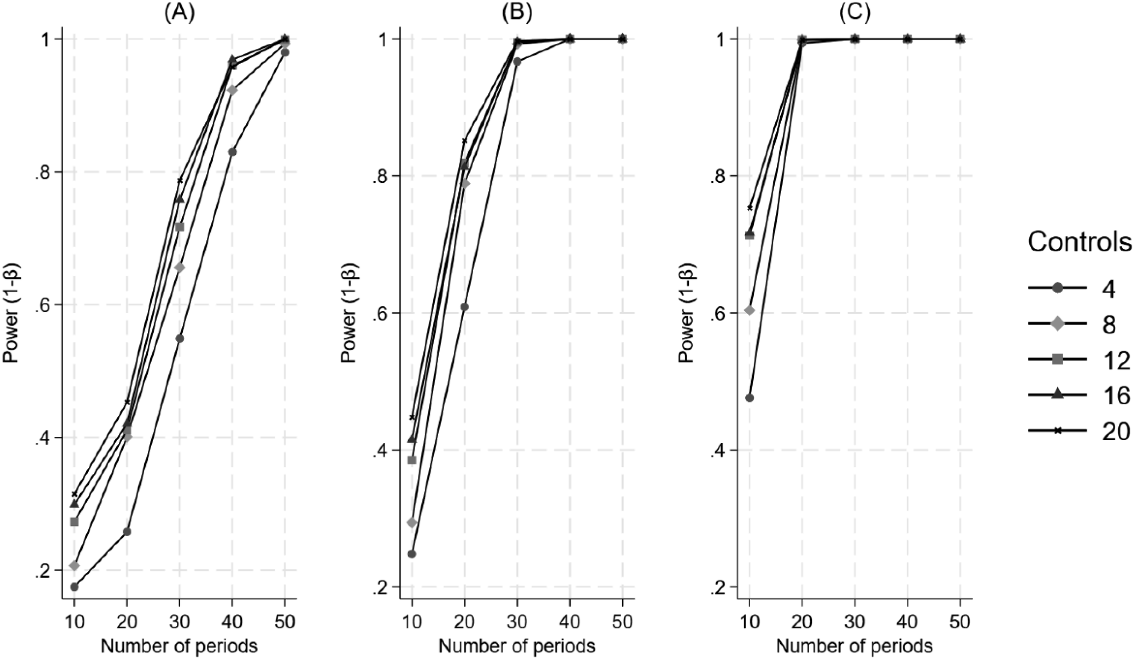

Figure 3 illustrates that when the treatment is introduced at a third of the time series, power increases monotonically as a function of an increasing number of control units and increasing effect size but requires an increasing number of time periods.

Figure 3

The Impact of the Number of Control Units and the Number of Time Periods on Power for a Difference in Differences in Trend, when the Treatment Begins at a Third of the Time Series. Panel A Represents a 25% Effect, Panel B Represents a 50% Effect, and Panel C Represents a 100% Effect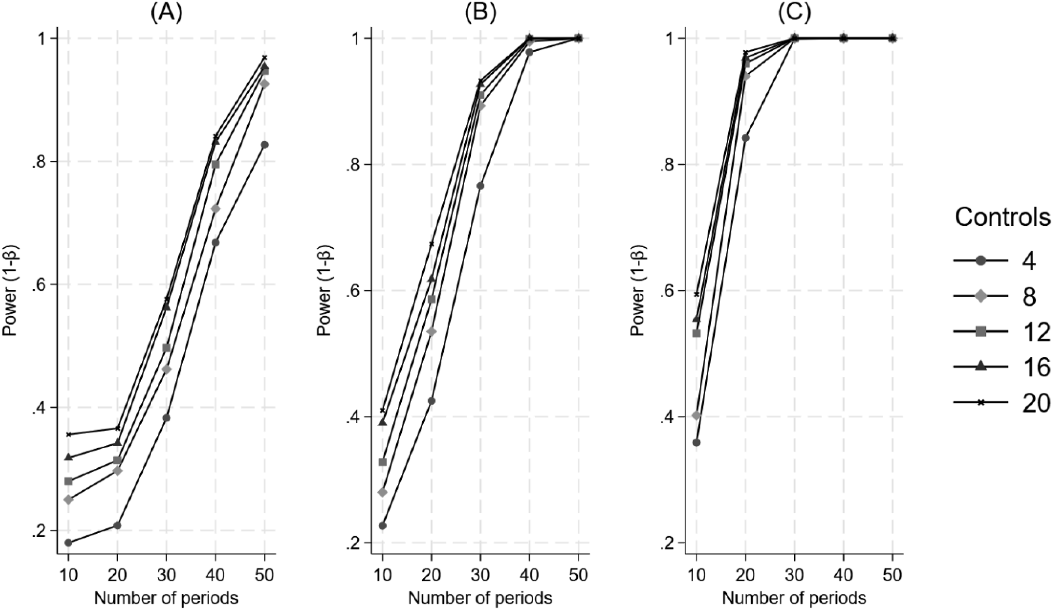

Figure 4 illustrates that when the treatment is introduced at two-thirds of the time series, the interaction between factors is similar to that of when the treatment is introduced at a third of the time series. That is, power increases monotonically as a function of an increasing number of control units and increasing effect size but requires an increasing number of time periods.

Figure 4

The Impact of the Number of Control Units and the Number of Time Periods on Power for a Difference in Differences in Trend, when the Treatment Begins at Two-Thirds of the Time Series. Panel A Represents a 25% Effect, Panel B Represents a 50% Effect, and Panel C Represents a 100% Effect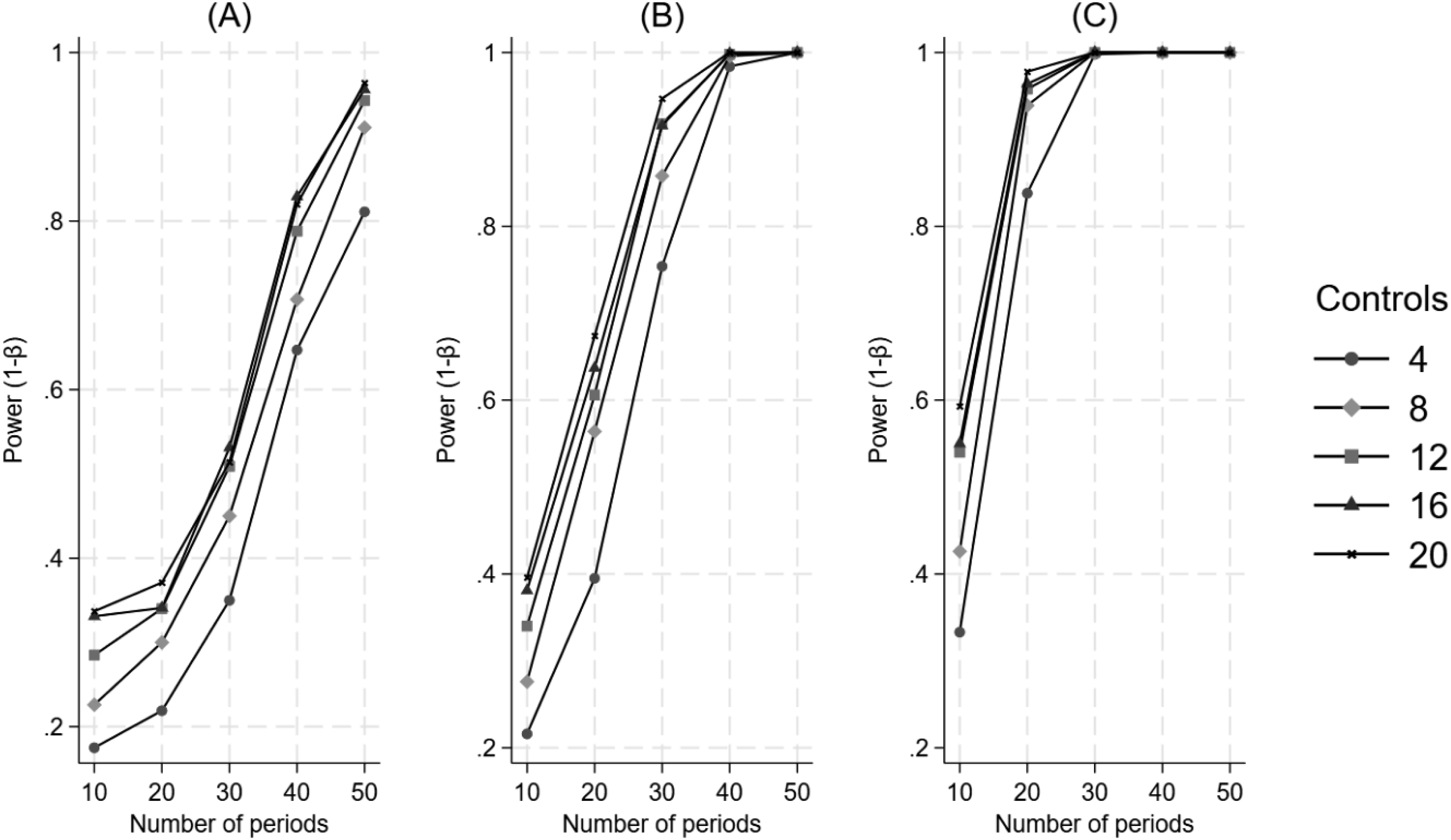

Appendix Figure 1 shows a direct comparison of power curves for when the treatment is introduced at a third, a half and two-thirds of the time series. The number of controls was set to 12 while all other input values were set as in the base scenario for difference in differences in trend. We see that power is consistently higher when the treatment is introduced at the halfway mark in the time series than when it is introduced earlier or later in the time series.

Figure 5 illustrates that increasing autocorrelation is associated with lower power, which remains consistent with an increasing number of time periods under study. There is a large amount of variability in the autocorrelation curves at a low effect size, and the patterns only become clear with a larger number of time periods.

Figure 5

The Impact of Varying Values of Autocorrelation and the Number of Time Periods on Power for a Difference in Differences in Trend. Panel A Represents a 25% Effect, Panel B Represents a 50% Effect, and Panel C Represents a 100% Effect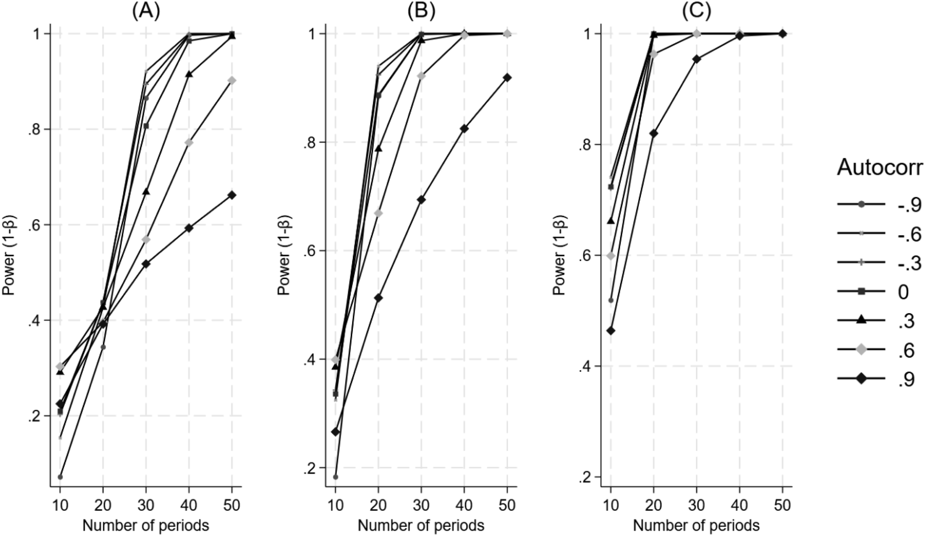

Difference in Differences in Level

Figure 6 illustrates that power increases consistently as a function of an increasing number of control units, an increasing number of time periods, and increasing effect size when the treatment is introduced at the halfway point in the time series.

Figure 6

The Impact of the Number of Control Units and the Number of Time Periods on Power for a Difference in Differences in Level, when the Treatment Begins at the Halfway Point in the Time Series. Panel A Represents a 20% Effect, Panel B Represents a 25% Effect, and Panel C Represents a 30% Effect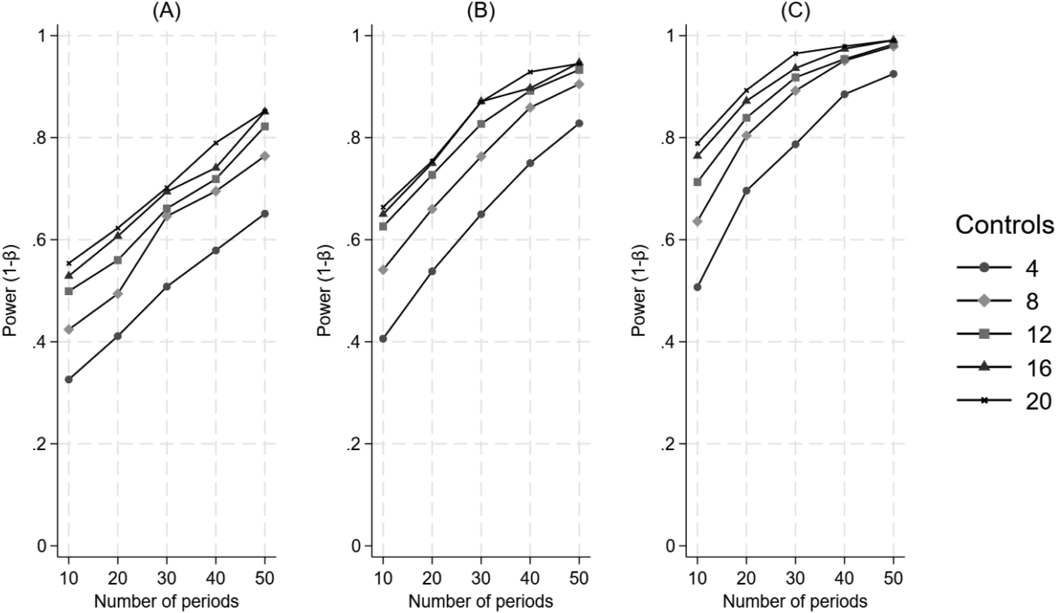

Figure 7 illustrates that power consistently increases as a function of an increasing number of control units, an increasing number of time periods, and increasing effect size when the treatment is introduced at a third of the time series. The behavior of the power curves is similar to those of when the treatment is introduced at the halfway mark in the time series.

Figure 7

The Impact of the Number of Control Units and the Number of Time Periods on Power for a Difference in Differences in Level, when the Treatment Begins at a Third of the Time Series. Panel A Represents a 20% Effect, Panel B Represents a 25% Effect, and Panel C Represents a 30% Effect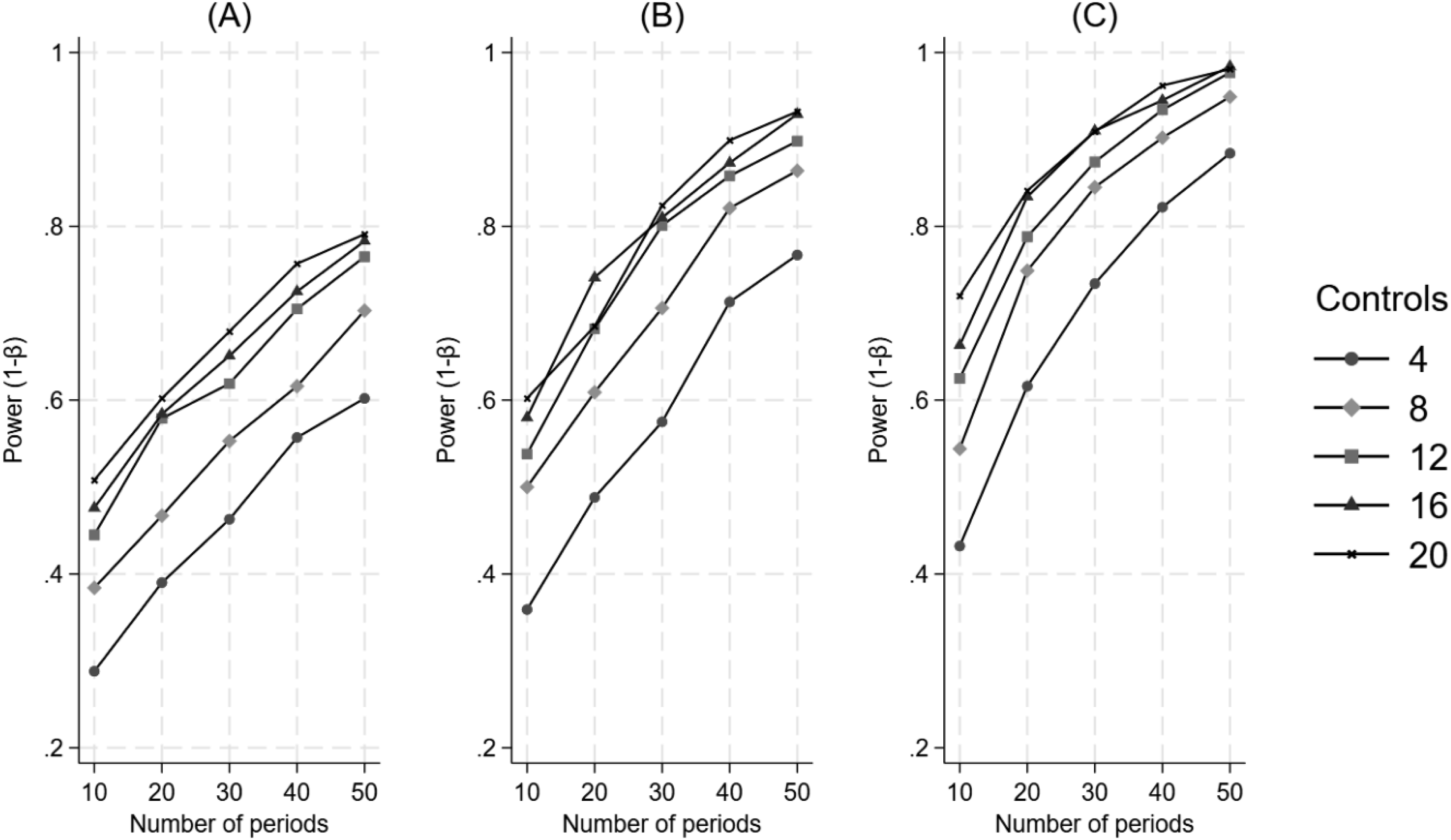

Figure 8 illustrates that the power curves, when the treatment is introduced at two-thirds of the time series, behave similarly to those when the treatment is introduced at a third of the time series. That is, power increases as a function of an increasing number of control units, an increasing number of time periods, and increasing effect size.

Figure 8

The Impact of the Number of Control Units and the Number of Time Periods on Power for a Difference in Differences in Level, when the Treatment Begins at a Two-Thirds of the Time Series. Panel A Represents a 20% Effect, Panel B Represents a 25% Effect, and Panel C Represents a 30% Effect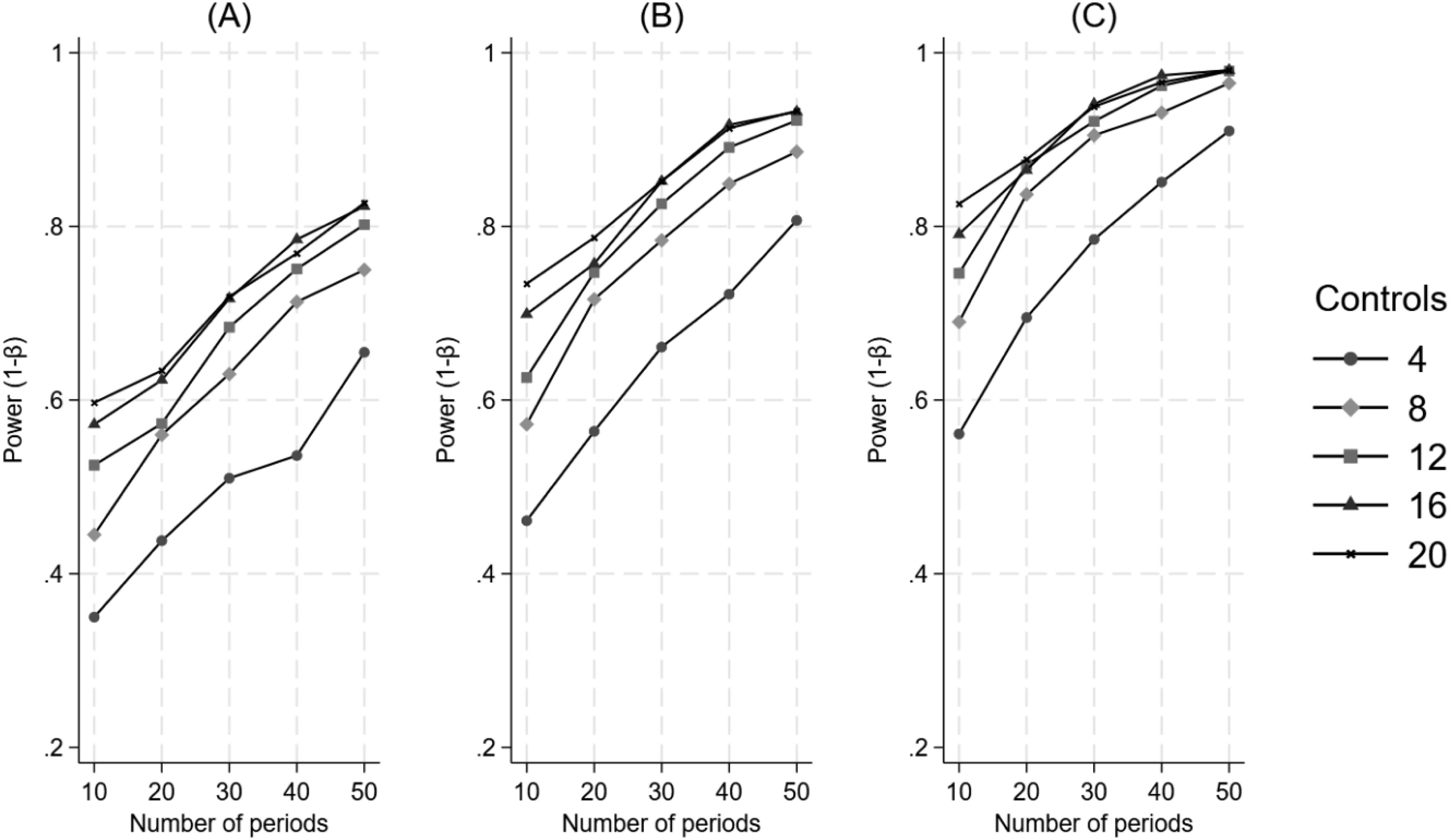

Appendix Figure 2 shows a direct comparison of power curves for when the treatment is introduced at a third, a half and two-thirds of the time series. The number of controls was set to 12 while all other input values were set as in the base scenario for difference in differences in level. We see little difference in power following an early or late intervention as compared to when the intervention occurred halfway through the time series.

Figure 9 illustrates an inconsistent relationship between autocorrelation and power, where the highest level of autocorrelation (0.9) is nearly flat regardless of the number of time periods, and the lowest level of autocorrelation (−0.9) how the lowest power of all the curves with the fewest time periods in the study and only appears to follow the path of the other curves at 15 time periods.

Figure 9

The Impact of Varying Values of Autocorrelation and the Number of Time Periods on Power for a Difference in Differences in Level. Panel A Represents a 20% Effect, Panel B Represents a 25% Effect, and Panel C Represents a 30% Effect

Appendix Figure 3 presents power curves for difference in differences in level when the treatment is introduced at the halfway point in the time series for effect sizes of 25% (reproduced from Figure 6) and 50%, to allow for a direct comparison with difference in differences in trend at 25% and 50% (Figure 2). In contrast to the difference in differences in trend, we see that generally fewer time periods are necessary to achieve power of 80%. For example, with a 25% effect size we see that at 30 time periods, the 3 largest control groups have surpassed 80% power for the difference in differences in level whereas it takes 40 time periods for the control groups to surpass 80% power for the difference in differences in trend. The gap widens between the two measures at 50% effect size where all control group sizes surpass 80% power within 10 time periods for the difference in differences in level, whereas it takes 30 time periods for all control group sizes to surpass 80% power in difference in differences in trend.

Sensitivity Analysis

Appendix Figures 4 and 5 present power curves for the sensitivity analysis of difference in differences in level and trend, respectively. The curves are consistent with those of the primary analyses illustrated in Figure 2 and in Figure 6, indicating that having different baseline levels or trends between treatment unit and controls does not affect power differently than when the groups share the same baseline level or trend.

Performance Analysis

Appendix Figures 6 and 7 present percentage bias estimates for difference in differences in level and trend, respectively. The percentage bias in both model coefficients was related to both the number of time periods and the effect size. Bias decreased as effect size increased and as the number of timer periods increased. The number of controls appears to differentially affect bias, with a larger number of controls exhibiting less bias.

Appendix Figures 8 and 9 present the bias estimates for difference in differences in level and trend at different levels of autocorrelation, respectively. For difference in differences in level, bias decreased as effect size increased and the number of time periods increased, with no differentiation between levels of autocorrelation. For difference in differences in trend, bias decreased as effect size increased, as the number of time periods increased, and with decreasing levels of autocorrelation. Overall, difference in differences in trend exhibited much more variability in bias than did the difference in differences in level.

Example

In this section we provide a worked example, using POWER_ITSA, to demonstrate how the simulation approach described herein can be tailored for a specific prospective research study, where the investigator wants to determine the number of control units and number of time periods necessary for a given effect size to achieve statistical significance.

Assume that a group of health services researchers are planning to conduct a longitudinal study in which one medical group will be given an artificial intelligence (AI) tool to assist in diagnosing patients’ ailments. Physicians will decide in which patient encounters they will employ the AI tool. The researchers hypothesize that the AI tool will reduce repeat office visits over time. 10 other medical groups will serve as controls and will not be given the AI tool. The researchers want to estimate how long the study should last in order to detect a statistically significant (p < 0.05) decrease in weekly office visits with at least 80% power. Since the study groups will be matched (and therefore comparable on baseline level and trend), the intercepts for both treatment unit and all control units are set to 500 weekly visits (their baseline level), and the pre-treatment trends of both treatment and control units are set to 0. However, the groups differ in the variability around the mean of their baseline time series, with the treated unit set to 2 standard deviations, and the control units’ set to 8 standard deviations. The researchers don’t expect to see a step change, since it will take time for the AI tool to achieve an effect. Therefore, the step option for both groups is also set to 0. The post-treatment trend for the control group is set to 0 since no change is expected in that group. However, the treated unit is expected to experience a decreased trend of 2 office visits per week (0.4%). We set the number of time periods to range from 10 to 20 weeks, in increments of 2. We set the treatment period to start at the halfway mark in the time series, and we specify that 2000 datasets for each time period (10 through 20) be simulated. We also set the level of autocorrelation at 0.20 for all units. This figure is derived from an analysis of existing time series data for the 11 groups using autocorrelation and partial autocorrelation functions (which are implemented in Stata using the AC and PAC commands). As shown in Appendix Figure 10, the results indicate that it will take about 16 weeks for the difference in differences in trend coefficient to achieve p < 0.05 at approximately 80% power (representing a total 6.4% decrease from the starting level). The investigators are also interested in estimating what effect size is needed to achieve 80% power assuming that the study was limited to only 10 weeks in total. As shown in Appendix Figure 11, we see that a reduction of 4 visits per week would be necessary to achieve 80% power at 10 weeks (holding all other input values at the same level as above).

Discussion

This novel study has identified several factors that a healthcare researcher must consider when determining the most efficient way to conduct an MG-ITSA study. The simulation results show that to increase power, a researcher can increase the number of control units, increase the number of time periods, focus on a difference in differences in level as the outcome of interest, start the treatment at the halfway mark in the time series (when testing the difference in differences in trend), and increase the effect size (or combinations of these factors). Autocorrelation is one aspect of an ITSA that cannot be readily manipulated by the researcher, and the simulation results show that increasing the amount of autocorrelation reduce power.

The finding of a direct association between an increasing number of control units and power has important implications for research studies using the MG-ITSA design. Holding all other factors constant, by simply increasing the number of control units, investigators can substantially reduce the overall length of the study to achieve the same power. This finding is intuitive given that the standard errors of the treatment effect coefficients (β₆ and β₇ in Equation (1)) get smaller with increasing sample size. In fact, the models with 12 control units produced standard errors for β₆ and β₇ that were about half the size as those for models with 4 control units, holding all other factors constant.

The explanation for why the difference in differences in level requires fewer time periods in a study to achieve the desired power than the difference in differences in trend lies in the fact that the coefficients representing the change in level focus on the period immediately following introduction of the treatment, resulting in a more easily detected signal when comparing against the pre-treatment level. Conversely, the change in trend is typically more subtle than the change in level, requiring more time periods to detect a signal. Taken together, this suggests that level changes are more readily detected in a study with a smaller number of time periods, and changes in trend are more likely detected as the number of time periods increase (Linden, 2025a).

For a study investigating the difference in differences in trend, introducing the treatment at the midpoint of the time series results in higher power than when the treatment begins either earlier or later in the time series. A likely explanation for this finding is that by balancing the number of time periods before and after the introduction of the treatment, the standard errors of the treatment effect estimates are minimized, thereby maximizing power (assuming no unusual factors impact the pre- and post-treatment periods differentially). This is a design efficiency analogous to why balanced groups maximize power in a two-group comparison (Van Belle, 2008).

Given the inverse relationship between effect size and study duration, investigators should strive to maximize effect size if reducing study length is important. In the worked Example, the effect size (a reduction of two office visits per week) was based on the fact that physicians decide whether and when to employ the AI tool. However, if the existing evidence indicates that the AI tool is effective in all patient encounters, the investigators could mandate its use for every visit. This would then allow them to assume a larger effect size, thereby shortening the overall duration of the study. In clinician-centered studies, the treatment effect could be enhanced by ensuring that sufficient training is provided to address potential cognitive biases and by asking physicians to commit to following the specific study protocols (Kullgren et al., 2017). In patient-centered studies, investigators should implement theory-based approaches to behavioral change to ensure that patients adhere to the treatment, thereby maximizing its effectiveness (Linden & Adler-Milstein, 2008; Linden et al., 2006). Additionally, investigators can potentially increase the size of treatment effects by maximizing the strength or dosage of the treatment, standardizing the treatment protocol, maintaining strong fidelity in treatment implementation, increasing the reliability in measuring treatment outcome, and taking steps to reduce error variance by holding constant or measuring (a) variations in treatment implementation and (b) irrelevancies in the treatment setting and treatment units.

From a statistical perspective, anticipating the level of autocorrelation is crucial. As the simulation results show for the difference in differences in trend, increasing autocorrelation results in lower power, holding the number of time periods, the number of controls, and the effect size constant. Given that only some of the lost power can be recovered through the use of time series regression, it is critical to obtain as accurate an estimate of autocorrelation as possible. If pre-study data are available, the investigator can review autocorrelation and partial autocorrelation functions (Box et al., 2016). One may ask how different levels of autocorrelation between the treatment unit and controls impact power? In a simple analysis of difference in differences in trend in which autocorrelation levels of −0.80, 0, and 0.80 were permuted for both the treatment unit and control units (for 4, 12, and 20 controls) and effect size was 25%, the results indicate that generally power is lowest when the control units’ autocorrelation is highest (0.80), regardless of what the treated unit’s autocorrelation was (Appendix Figure 12). This result is intuitive given that in an MG-ITSA power depends on how well the controls’ time series identify the counterfactual trend for the treated unit. High autocorrelation in the controls’ time series sharply inflates the variance, thereby reducing power to detect a treatment effect. Autocorrelation in the single treated unit matters far less because it affects only one time series and does not substantially impair estimation of the counterfactual. In the absence of any pre-treatment data the most practical advice may be to “over-correct” for the expected level of autocorrelation when planning the study. For example, the investigator can assume a higher level of autocorrelation and plan to extend the study for the number of time periods necessary to elicit the desired power. Alternatively, one can simply apply a range of autocorrelations in the power computations and determine where the tradeoff is between the various factors that can be manipulated and autocorrelation, which cannot. The effect of autocorrelation on power was less clear for the difference in differences in level (Figure 9). This may also be related to fact that the difference in differences in level measures the change in the time series for a single time period whereas the difference in differences in trend measures the change in the time series over a number of time periods. Naturally, the effects of autocorrelation are harder to detect for a single observation than when measured over a larger number of observations.

Given that autocorrelation cannot be directly manipulated as a study element, it must be controlled for in the time series regression model used to estimate treatment effects. In the current paper, power was computed using OLS regression adjusted with Newey-West standard errors (Newey & West, 1987), however many other time series regression models are available, such as Prais-Winsten (Prais & Winsten, 1954), Cochrane-Orcutt (Cochrane & Orcutt, 1949), and any one of the autoregressive conditional heteroskedasticity (ARCH) family of estimators, among others (see Harvey [1989] and Enders [2004] for a comprehensive discussion of econometric time series models). A general limitation of these models is that they are unduly complex and unapproachable for non-econometricians. Conversely, an OLS estimator with Newey-West standard errors requires no specialized training, and the interpretation of coefficients is straight-forward.

While the current paper includes figures for investigators that are based on general guidance related to the various components of power and their interactions, the simulation methods implemented here can be tailored to use specific inputs, much in the same way that empirically-driven power calculations are used for generating estimates. This was demonstrated in the worked example. The community-contributed Stata package POWER_ITSA (Linden, 2025b) allows researchers to replicate the results of the simulation study and the worked example, as well as design their own power analyses.

The strength of this study lies in its comprehensive simulation strategy, in which every input variable was manipulated to some degree, with the exception of the variability (noise) infused in the control units’ time series (the controls were set to 2 SD and the treated unit was set to 1 SD, throughout). Increased variability in the controls time series relative to that of the treated unit functionally reduces power, so the simulations here could have been idealized by setting both treated and control units to have the same amount of variability in their time series. However, the present design is more aligned with what researchers can expect in real MG-ITSA data where potential controls may have comparable mean baseline level and trend to that of the treated unit, but more variability around those estimates. Taken together, the results presented here are likely to generalize to most MG-ITSA conditions.

These findings offer practical guidance for health professionals designing MG-ITSA studies. Clinicians and quality improvement leaders can prospectively plan study duration and comparator selection and health services researchers benefit from knowing that additional control units substantially increase power, often enabling shorter study periods and faster translation to practice.

The present study has limitations. The simulation strategy developed here was designed to replicate the most common MG-ITSA study in healthcare research: a single treatment-group compared to 2 or more control units with a single treatment (treatment) period, in which OLS time series regression is used as the statistical model and assumes a first-order autocorrelation (lag = 1) for both treatment and control units, and handles the outcome variable as continuous (regardless of true data type). This implies that several factors were not included in the simulation design: multiple consecutive treatments, seasonality, higher-order autocorrelation, and different outcome variable types. Generally, when there is suspected seasonality in the data and it cannot be modeled directly at the design stage, investigators should err on the side of increasing the length of the study, as the minimum required sample size increases with variability, model complexity, and seasonal period length (Hyndman & Kostenko, 2007). When other factors appear to impact the time series, the investigator should attempt to model them at the design stage of the simulations to get the most accurate estimates of power. Finally, OLS regression was the underlying statistical model used here for estimating power via simulation. Future research should investigate how power estimates for MG-ITSA studies compare when different modeling approaches are considered, such as other time series regression models (e.g. ARCH), autoregressive integrated moving average (ARIMA) models for interventions (Box & Tiao, 1976), Bayesian frameworks (Ma & Benmarhnia, 2025), instrumental variables (Linden & Adams, 2006), and machine learning algorithms (Linden & Yarnold, 2018).

Conclusion

Based on the results of a comprehensive set of simulations, this novel study provides guidance on estimating power in MG-ITSA studies for which OLS time series regression will be used as the statistical model. Healthcare researchers must consider the many factors highlighted here that uniquely affect power when determining the most efficient way to conduct an MG-ITSA study.

Supplemental Material

Suppplemental Material - Power Considerations for Multiple-Group (Controlled) Interrupted Time Series Analysis: A Comprehensive Simulation Study

Suppplemental Material for Power Considerations for Multiple-Group (Controlled) Interrupted Time Series Analysis: A Comprehensive Simulation Study by Ariel Linden in Evaluation & the Health Professions

Footnotes

Funding

The author received no financial support for the research, authorship, and/or publication of this article.

Declaration of conflicting interests

The author declared no potential conflicts of interest with respect to the research, authorship, and/or publication of this article.

Supplemental Material

Supplemental material for this article is available online.

References

Abadie

Diamond

Hainmueller

(2010). Synthetic control methods for comparative case studies: Estimating the effect of California’s tobacco control program. Journal of the American Statistical Association, 105(490), 493–505. https://doi.org/10.1198/jasa.2009.ap08746

Ansermino

J. M.

Pillay

Tagoola

Zhang

Dunsmuir

Kamau

Kigo

Agaba

Aye

I. A.

Hwang

Novakowski

S. K.

Huxford

Wiens

M. O.

Kimutai

Ouma

Ahmed

Mwaniki

Oyella

Tenywa

, …, & Pediatric Sepsis CoLab . (2025). Implementation of smart triage combined with a quality improvement program for children presenting to facilities in Kenya and Uganda: An interrupted time series analysis. PLOS Digital Health, 4(3), Article e0000466. https://doi.org/10.1371/journal.pdig.0000466

Aye

T. T.

Nguyen

H. T.

Petitfour

Ridde

Amberg

Bonnet

Seynou

Kiendrébéogo

J. A.

De Allegri

(2025). How do free healthcare policies impact utilization of maternal and child health services in fragile settings? Evidence from a controlled interrupted time series analysis in Burkina Faso. Health Policy and Planning, 39(9), 891–901. https://doi.org/10.1093/heapol/czae077

Barbalat

De Rozario

Franck

(2025). Reducing mental health emergency department visits through community-based assessment services. A controlled time-series analysis in the city of Lyon, France. Health Policy, 161, Article 105419. https://doi.org/10.1016/j.healthpol.2025.105419

Box

G. E. P.

Jenkins

G. M.

Reinsel

G. C.

Ljung

G. M.

(2016). Time series analysis: Forecasting and control (5th ed.). Wiley.

Box

G. E. P.

Tiao

G. C.

(1976). Intervention analysis with applications to economic and environmental problems. Journal of the American Statistical Association, 70(349), 70–79. https://doi.org/10.1080/01621459.1975.10480264

Burton

Altman

D. G.

Royston

Holder

R. L.

(2006). The design of simulation studies in medical statistics. Statistics in Medicine, 25(24), 4279–4292. https://doi.org/10.1002/sim.2673

Campbell

D. T.

Stanley

J. C.

(1966). Experimental and quasi-experimental designs for research. Rand McNally.

Cochrane

Orcutt

G. H.

(1949). Application of least squares regression to relationships containing auto-correlated error terms. Journal of the American Statistical Association, 44(245), 32–61. https://doi.org/10.2307/2280349

10.

Liu

Yang

(2025). How DRG payment reform shapes inpatient neurological care in an underdeveloped region: Evidence from a controlled interrupted time series study in Yunnan, China. Risk Management and Healthcare Policy, 18, 2575–2590. https://doi.org/10.2147/RMHP.S530693

11.

Dziak

J. J.

Dierker

L. C.

Abar

(2020). The interpretation of statistical power after the data have been gathered. Current Psychology, 39(3), 870–877. https://doi.org/10.1007/s12144-018-0018-1

12.

Enders

(2004). Applied econometric time series (2nd ed.). Wiley.

13.

Fanshawe

T. R.

Turner

P. J.

Gillespie

M. M.

Hayward

G. N.

(2022). The comparative interrupted time series design for assessment of diagnostic impact: Methodological considerations and an example using point-of-care C-reactive protein testing. Diagnostic and Prognostic Research, 6(1), 3. https://doi.org/10.1186/s41512-022-00118-w

14.

Gressler

Lewis

(2025). Changes in maternal morbidity and infant outcomes following state-level abortion bans post-Dobbs: A comparative interrupted time series study. BMC Public Health, 25(1), 2265. https://doi.org/10.1186/s12889-025-23468-8

15.

Harvey

A. C.

(1989). Forecasting, structural time series models and the kalman filter. Cambridge University Press.

16.

Hawley

Ali

M. S.

Berencsi

Judge

Prieto-Alhambra

(2019). Sample size and power considerations for ordinary least squares interrupted time series analysis: A simulation study. Clinical Epidemiology, 11, 197–205. https://doi.org/10.2147/CLEP.S176723

17.

Hyndman

R. J.

Kostenko

A. V.

(2007). Minimum sample size requirements for seasonal forecasting models. Foresight, 6(Spring), 12–15.

18.

Kullgren

J. T.

Krupka

Schachter

Linden

Miller

Acharya

Alford

Duffy

Adler-Milstein

(2018). Precommitting to choose wisely about low-value services: A stepped wedge cluster randomised trial. BMJ Quality and Safety, 27(5), 355–364. https://doi.org/10.1136/bmjqs-2017-006699

19.

Kutner

M. H.

Nachtsheim

C. J.

Neter

(2005). Applied linear statistical models. McGraw-Hill Irwin.

20.

Landau

Stahl

(2013). Sample size and power calculations for medical studies by simulation when closed form expressions are not available. Statistical Methods in Medical Research, 22(3), 324–345. https://doi.org/10.1177/0962280212439578

21.

Linden

(2013). Assessing regression to the mean effects in health care initiatives. BMC Medical Research Methodology, 13, 1–7, Article 119. https://doi.org/10.1186/1471-2288-13-119

22.

Linden

(2015). Conducting interrupted time-series analysis for single-and multiple-group comparisons. STATA Journal, 15(2), 480–500. https://doi.org/10.1177/1536867X1501500208

23.

Linden

(2017a). Challenges to validity in single-group interrupted time series analysis. Journal of Evaluation in Clinical Practice, 23(2), 413–418. https://doi.org/10.1111/jep.12638

24.

Linden

(2017b). Persistent threats to validity in single-group interrupted time series analysis with a crossover design. Journal of Evaluation in Clinical Practice, 23(2), 419–425. https://doi.org/10.1111/jep.12668

25.

Linden

(2017c). A comprehensive set of postestimation measures to enrich interrupted time-series analysis. STATA Journal, 17(1), 73–88. https://doi.org/10.1177/1536867X1701700105

26.

Linden

(2018). A matching framework to improve causal inference in interrupted time‐series analysis. Journal of Evaluation in Clinical Practice, 24(2), 408–415. https://doi.org/10.1111/jep.12874

27.

Linden

(2022). Erratum: A comprehensive set of postestimation measures to enrich interrupted time-series analysis. STATA Journal, 22(1), 231–233. https://doi.org/10.1177/1536867X221083929

28.

Linden

(2025a). A comprehensive simulation study to evaluate the effect size and study length relationship in single-group interrupted time series analysis. Evaluation & the Health Professions, Article 01632787251361514. https://doi.org/10.1177/01632787251361514

29.

Linden

(2025b). POWER_ITSA: Stata module to compute power for single and multiple-group interrupted time series analysis. In: Statistical software components (S459461). Boston College Department of Economics.

30.

Linden

Adams

J. L.

(2006). Evaluating disease management programme effectiveness: An introduction to instrumental variables. Journal of Evaluation in Clinical Practice, 12(2), 148–154. https://doi.org/10.1111/j.1365-2753.2006.00615.x

31.

Linden

Adler-Milstein

(2008). Medicare disease management in policy context. Health Care Financing Review, 29(3), 1–11.

32.

Linden

Butterworth

S. W.

Roberts

(2006). Disease management interventions II: What else is in the black box? Disease Management, 9(2), 73–85. https://doi.org/10.1089/dis.2006.9.73

33.

Linden

Yarnold

P. R.

(2016). Using machine learning to identify structural breaks in single-group interrupted time series designs. Journal of Evaluation in Clinical Practice, 22(6), 855–859. https://doi.org/10.1111/jep.12544

34.

Linden

Yarnold

P. R.

(2018). Using machine learning to evaluate treatment effects in multiple‐group interrupted time series analysis. Journal of Evaluation in Clinical Practice, 24(4), 740–744. https://doi.org/10.1111/jep.12966

35.

Luo

Zhao

Yao

Liu

(2025). Reducing proton pump inhibitors overuse with an advisory, risk-based, context-aware electronic alert system: A controlled interrupted time series analysis. International Journal of Medical Informatics, 202, Article 105960. https://doi.org/10.1016/j.ijmedinf.2025.105960

36.

Benmarhnia

(2025). Interrupted time series analysis in environmental epidemiology: A review of traditional and novel modeling approaches. Current Environmental Health Reports, 12(1), 50. https://doi.org/10.1007/s40572-025-00517-3

37.

Newey

W. K.

West

K. D.

(1987). A simple, positive semi-definite, heteroskedasticity and autocorrelation consistent covariance matrix. Econometrica, 55(3), 703–708. https://doi.org/10.2307/1913610

38.

Power

Tyrrell

P. J.

Rudd

A. G.

Tully

M. P.

Dalton

Marshall

Parry

Corgié

Goldmann

Webb

Dixon-Woods

(2014). Did a quality improvement collaborative make stroke care better? A cluster randomized trial. Implementation Science, 9(1), 40. https://doi.org/10.1186/1748-5908-9-40

39.

Prais

S. J.

Winsten

C. B.

(1954). Trend estimators and serial correlation. Discussion Paper 383, Cowles Commission.

40.

Rubin

D. B.

(1974). Estimating causal effects of treatments in randomized and non-randomized studies. Journal of Educational Psychology, 66(5), 688–701. https://doi.org/10.1037/h0037350

41.

Schochet

P. Z.

(2022). Statistical power for estimating treatment effects using difference-in-differences and comparative interrupted time series estimators with variation in treatment timing. Journal of Educational and Behavioral Statistics, 47(4), 367–405. https://doi.org/10.3102/10769986211070625

42.

Shadish

W. R.

Cook

T. D.

Campbell

D. T.

(2002). Experimental and quasi-experimental designs for generalized causal inference. Houghton Mifflin.

43.

Tsunemitsu

Shin

J. H.

Hamada

Tsutsumi

Sasaki

Kunisawa

Imanaka

(2025). Effects of protocol-driven care by internists on adherence to clinical practice guidelines for hip fracture surgery patients: An interrupted time series study using a nationwide inpatient database. Internal Medicine, 64(14), 4358–4424. https://doi.org/10.2169/internalmedicine.4358-24

44.

Van Belle

(2008). Statistical rules of thumb (2nd ed.). Wiley & Sons.

45.

Walter

S. R.

Salisbury

Scott

L. J.

de Vocht

Macleod

Ben-Shlomo

Curtis

H. J.

Sheikh

Katikireddi

S. V.

Mehrkar

Bacon

Hickman

Goldacre

Redaniel

M. T.

OpenSAFELY Collective . (2025). The impact of COVID-19 lockdowns on primary care contact among vulnerable populations in England: A controlled interrupted time series study. British Journal of General Practice Open, 9(4). https://doi.org/10.3399/BJGPO.2025.0017

46.

Wanigaratne

Stukel

Guan

Hynie

Saunders

N. R.

Guttmann

(2025). Morbidity among resettled refugees at arrival in Ontario, Canada (1994–2017): A controlled interrupted time series study examining the effect of the immigration refugee protection act, 2002. Journal of Epidemiology & Community Health, 79(4), 249–256. https://doi.org/10.1136/jech-2024-222947

47.

Wyper

Mackay

D. F.

Fraser

Lewsey

Robinson

Beeston

Giles

(2023). Evaluating the impact of alcohol minimum unit pricing on deaths and hospitalisations in Scotland: A controlled interrupted time series study. Lancet, 401(10385), 1361–1370. https://doi.org/10.1016/S0140-6736(23)00497-X

48.

Yelland

Riggs

Szwarc

Casey

Dawson

Vanpraag

Brown

Wallace

Teale

Harrison

Petschel

Furler

Goldfeld

Mensah

Biro

M. A.

Willey

Cheng

I. H.

Small

(2015). Bridging the gap: Using an interrupted time series design to evaluate systems reform addressing refugee maternal and child health inequalities. Implementation Science, 10, Article 62. https://doi.org/10.1186/s13012-015-0251-z

49.

Zhang

Wagner

A. K.

Ross-Degnan

(2011). Simulation-based power calculation for designing interrupted time series analyses of health policy interventions. Journal of Clinical Epidemiology, 64(11), 1252–1261. https://doi.org/10.1016/j.jclinepi.2011.02.007

Supplementary Material

Please find the following supplemental material available below.

For Open Access articles published under a Creative Commons License, all supplemental material carries the same license as the article it is associated with.

For non-Open Access articles published, all supplemental material carries a non-exclusive license, and permission requests for re-use of supplemental material or any part of supplemental material shall be sent directly to the copyright owner as specified in the copyright notice associated with the article.

0.00 MB

0.68 MB