Nonlinear dynamical behavior of a three-degree-of-freedom asymmetric rigid body under gyroscopic torque

Abstract

The study in this paper focuses on solving the problem of rigid body (RB) rotary motion under the effect of both gyrostatic torque (GT) and the body’s constant fixed torques (BCFTs). The controlling equations of motion (EOMs), in such a case, are derived from Euler’s kinematic equations. Novel analytical solutions for the body angular velocities are approached in three instances: major, minor, and intermediate with a detailed description of the stability regions, equilibrium points (EPs), and the motion critical points. The extreme value of the case is also examined, with stabilization addressed in two sections. Each section offers a solution and includes a table of extreme values within the stable separatrix region. Additionally, the effect of distinct GT values on the motion’s paths and stabilization is analyzed, resulting in valuable insights for this scenario. For each case, a comprehensive estimation of the maximum values and minimum ones at distinct non-dimensional angular velocity components (NAVCs) in addition to periodic solutions has been approached. A contour mapping for the motion is presented to see the influence of the GT on the separatrix surfaces (SS), non-periodic or periodic solutions, and extreme periodic ones. Moreover, a three-dimensional (3D) representation of the numerical solution in the intermediate case was presented to also reveal the GT impact. The significant implications of these findings are clear in systems’ designing and evaluation utilizing asymmetric RBs, such as spaceships. This research could inspire further exploration of different perspectives within the GT in comparable scenarios, potentially impacting numerous fields, such as the engineering industry and navigation.

Introduction

The rotary motion of RBs, particularly when influenced by GT, is a complex yet fascinating area of study in dynamics and mechanical engineering. The GT, which arises from the angular momentum of rotating systems, plays a crucial role in stabilizing and controlling the motion of various mechanical and aerospace structures. When the RB experiences this torque, its rotational behavior exhibits unique characteristics, often leading to phenomena such as precession and nutation. Understanding these effects is essential for the design and operation of gyroscopes, spinning satellites, and other rotational devices. This study delves into the principles governing the gyrostatic effects on RBs, providing insights into their practical applications and theoretical underpinnings. In addition to a solution for such a problem in three distinct cases, the governing EOMs for such a problem are given by Euler’s equations^1,2 and the RB’s orientation for a constrained problem ³ . A study is conducted on the rotary movement of asymmetric RB when impacted by a stationary torque ⁴ and with a GT ⁵ . The focus is on developing 3D phase space paths for three scenarios: BCFTs along the major axis, BCFTs along the minor axis, and BCFTs along the central axis. These studies present novel analytical and numerical simulated findings for each case, including SS, EPs, periodic or non-periodic solutions, and the motion critical points. In ⁶ , the authors have successfully obtained analytical solutions for the EOMs under conditions that align with the physical characteristics of the body. The solution’s uniqueness is demonstrated in the presence of GT. Furthermore, novel theoretical applications are introduced for cases where the body exhibits symmetrical about one of its principal axes and when it is entirely symmetric. In ⁷ , the study investigates the motion of a charged RB having a spherical cavity filled with an incompressible viscous liquid. Factors such as the GT, BCFTs, and the torque from a resistant force, influenced by the liquid’s shape, are taken into account. The averaging method is employed to derive a suitable form of the governing system for EOMs. Taylor’s method is then utilized to solve the averaged EOMs for the RB, considering various initial conditions to achieve the desired outcomes. The asymptotic approach of the averaged system, combined with numerical analysis, facilitates the attainment of appropriate results for the problem. In ⁸ , the study investigates the dynamics of a charged axisymmetric RB in the presence of GT. The effects of transverse and BCFTs are examined. By using small angular approximation, approximate novel solutions are derived for the attitude and examined motion. These concise, complex-form responses are quite useful for deciphering the actions performed by spinning RBs. In^9,10, the study is focused on the symmetric RB’s motion about one of the main axes in the existence of a Newtonian force field (NFF) and a GT with a second component equal to zero ⁹ and the absence of the NFF ¹⁰ . The assumption is restricted that the body’s center of mass is slightly displaced relative to the dynamic axis of symmetry. The periodic solutions and Euler angles for irrational frequencies’ cases are achieved at any given time.

In ¹¹ , novel analytical solutions are presented for the rotary motion of RB with two equal principal inertia moments, under the influence of a stationary external torque. The following scenarios have solutions derived just for them; firstly, when the starting angular velocity is random and the torque is supposed to be parallel to the symmetry axis; secondly, when the torque rotates about the symmetry axis at a stationary rate with an arbitrary initial angular velocity while it is perpendicular to the symmetry axis; thirdly, when the starting angular velocity and torque are both orthogonal to the symmetry axis, and the torque stays stationary with the RB. In ¹² , the averaging method of Krylov–Bogoliubov is employed. It has been shown in ¹³ that problems involving the dynamics of an RB with a viscous fluid can be broken down into two separate categories: dynamic and hydrodynamic. The authors examine the rotation of almost spherical RB with a cavity full of a viscous liquid. The body is subjected to BCFTs while considering asymptotic approximations of the torques of the viscous fluid. The estimation of the body’s motion under the influence of small internal and external torques is described through solutions obtained from numerical and analytical calculations conducted over the time interval. In ¹⁴ , the authors introduce a novel solving procedure applicable to all equations, including the momentum equation of a charged RB influenced by the Lorentz force in the non-relativistic scenario.The study ¹⁵ concentrates on using non-dimensional variables to achieve the time-optimal slowing of a dynamically asymmetric RB, which allowed for the derivation of a multi-parameter system of EOMs. Constructing a vector hodograph of the angular momentum in 3D space involves varying the system parameters. According to the study’s outcomes, certain ratios between the problem’s parameters are necessary to get the best possible RB deceleration. In ¹⁶ , the study examines the movement of a closely spherical RB with a viscoelastic component. The dynamics of the RB around the mass center, where viscoelasticity arises from the movement of mass linked by spring-dampers to points on the main axes is investigated. Numerical integration of asymptotic EOMs is performed to analyze the body’s motion, yielding solutions over an infinite period with asymptotically small errors. In ¹⁷ , an analytical technique is proposed, grounded in the identification of failure mechanisms. Initially, a forensic survey is conducted on two typical cases of overturning, culminating in the identification and summary of three typical overturning failure modes along with their respective criteria for evaluating failure. Subsequently, the analytical technique is developed under the assumption that the girder’s overturning involves both RB and deformable body rotations, taking into account characteristics such as radial bending and torsional deformation. In ¹⁸ , a novel procedure is introduced to determine the coordinates of the infinitesimal body with its orbit positioned close to a planet. A system of EOMs is utilized to derive analytic and semi-analytic solutions. Two Cartesian coordinates are shown to be dependent on the genuine anomaly and a function that determines whether the solution is quasi-periodic, while the third coordinate shows quasi-periodic fluctuations. In ¹⁹ , the GT and the BCFTs are the two external torques that affect the RB’s rotation. In order to decouple and solve the governing EOMs in a complex form, the authors have been developed and scaled these equations. A software has been used to approach and illustrate the new analytical approaches for the angular velocities. In ²⁰ , the primary torques of inertia are thought to correlate to a basic algebraic equivalence. Furthermore, the selection of the first condition is constrained. Using the same software in ¹⁹ , the problem’s analytical solution is presented and graphically represented.

In ²¹ , the author investigates the dynamics of a system comprising two RBs connected by a cylindrical hinge. While there are no rotors involved, a control element in the form of a latch is present, capable of securing the rotor’s position. Various attitude control tasks are explored, including the gyrostat’s flipping. In ²² , the authors address the motion of a gyrostat influenced by potential and gyroscopic forces, particularly when its GT varies. The study delves into the conditions necessary for the existence of linear invariant relations within Kirchhoff-Poisson’s equations. Additionally, a novel solution to these equations is derived regarding the elementary functions. In ²³ , investigations are conducted into perturbed rotational movements of the RB, which are comparable to normal precession in the Lagrange scenario, where the restoring torque is dependent on the angle of nutation. The perturbed rotational movements of the RB near regular precession in Lagrange scenario are studied again in ²⁴ but the authors made three restrictions on the problem regarding the angular velocity, the dynamic symmetry axis, and the perturbation moment. For the same problem again, in ²⁵ , the acceleration approach is applied, and a small parameter is added in a unique way. The first and second approximations yield averaged systems of motion equations. The second approximation determines the development of the precession angle. In ²⁶ , a virtually dynamically spherical RB with a viscoelastic component is examined in its rotatory motion. A moving mass attached to a location on one of the primary axes of inertia via a spring and damper simulates this element. In ²⁷ , The movement of a nearly symmetrical RB subject to BCFTs about three axes is studied and approximate real analytic solutions are obtained. Fresnel integrals are used to give the exact solution to Euler’s equations of motion for symmetric bodies. In ²⁸ , using Euler’s angles, the author has shown an elegantly analytical instance of rotations of the general kind in a fixed Cartesian coordinate system. In ²⁹ , the authors have examined a disturbed motion that is similar to the Lagrange situation, accounting for tiny and constant dissipative torques as well as dissipative torques that vary on slow time. In ³⁰ , the authors have extended their work on earlier findings about the dynamic motion of symmetric RB under perturbation and restoring torques. The average method has been used to simplify the EOMs and latterly approach a solution for the problem. In ³¹ , an almost spherical RB with a hollow interior filled with a very viscous fluid and exposed to BCFTs is examined in terms of its motion about its center of mass. While the liquid dynamics is addressed by 3D Navier–Stokes equations which has been transformed into two Riccati solved equations ³² . In ³³ , the authors have derived a fourth first integral for the motion in the three well-known cases while the GT has taken action on the RB orientation. In ³⁴ , for Euler–Poinsot case, the problem has been investigated and solved for the RB orientating in the NFF and impacted by GT. In ³⁵ , for a similar model in an NFF, Poincare small parameter method is used to solve the problem with the impact of the third component of the GT only. In ³⁶ , the perturbed rotary motion of a gyrostat about a fixed point with mass distribution near to Lagrange’s case is investigated. The method presented in ³⁷ enables us to arrive at all of the equations that any RB shifting arbitrarily in 3D space has to fulfill in a logical and ordered manner. In ³⁸ , for the scenario of a symmetric RB, the authors obtain the sum of the Cauchy–Kovalevskaya series. They derive the solution to the EOMs for the RB in terms of elementary functions by employing the integrals of motion and directly adding the elements of these series. The study ³⁹ examines the analytical approach for rotational movement when a motor with limited power is present. The goal is to demonstrate that, regardless of the variables of the issue and the beginning circumstances, the carrier body’s movement approaches revolution around an axis that is stationary.

Some lately published works on the problem dealing with the applications of the problem in spacecrafts, satellites, and asteroids have been investigated in^40–48. In ⁴⁰ , the case of a spacecraft subjected to a time-dependent temperature field has led to a revisitation of the traditional Euler–Poisson’s EOMs that describe the movement of RB about the stationary point. While a new study has investigated the effects of energy dissipation ⁴¹ and the response of a spacecraft to GT and BCFTs ⁴² while it contains a slug has also been derived. In ⁴³ , the presence and stability of periodic orientation close to hyperbolic precession for a symmetric RB with an elliptical orbiting center of gravity are the main topic of the research. In ⁴⁴ , the attitude development of a spacecraft loaded with dual liquids and undergoing internal energy dissipation is examined. In order to investigate several trajectories, such as major axis spin, period-n limit cycle, and chaotic motion, the spacecraft system’s dynamic equations are created. Melnikov’s technique provides a criterion for predicting when the system may experience chaotic motion. In ⁴⁵ , for an axi-symmetrical satellite model impacted by the GT and orientating in both NFF and electromagnetic one with also its center of gravity shift from the symmetrical axis, the small parameter method of Poincare has been used to approach a solution for the problem in the irrational frequencies case. In ⁴⁶ , it is demonstrated that, subject to a restriction on the Euclidean norm of the applied torque, the anti-parallel approach is the best course for spaceship collapse. The solution is validated for lengthy maneuver periods and extremely asymmetric spacecraft by comparisons to a numerically integrated optimum control rule. Any asymmetric spacecraft’s rest-to-rest reorientation maneuver may be analytically expressed by combining the parallel and anti-parallel torque solutions. In ⁴⁷ , in order to describe the physically plausible response of a “rubble pile” of asteroid volumetric material to the action of a projectile impacting its surface, the authors have examined a novel particular model for the dynamics of a non-rigid asteroid rotation. This model assumes the added mass model rather than the concept of Viscoelastic Oblate Rotators. In ⁴⁸ , the outermost layer of a magnetically induced asteroid with a predominantly conducting structure has been observed to have a novel physical effect that is physically self-consistent to consider when further calculating the dynamics of asteroid rotation. Normally, an asteroid with a predominantly metallic formation is thought to be moving in the planet’s external magnetic field while orbiting, ideally, outside its sphere of effective attraction. These pervious works have proved the various applications of the problem in aerospace engineering, navigation, and control.

In this paper, analytical solutions for the RB’s motion affected by the GT and BCFTs are presented. Euler’s EOMs are scaled and nondimensionalized for BCFTs, identifying EPs, linearized EOMs, stability characteristics, and characteristic equations. For BCFTs along major and minor axes, analytical solutions are obtained through comprehensive simulations, elucidating steady states, paths, stability regions, and extreme values. BCFT along the central axis is addressed with a numerical solution, displaying 3D and 2D graphs of NAVCs, showcasing typical spin-up maneuvers and stability shifts with varying GT. The study also examines extreme cases, providing solutions and tables of extreme values, while analyzing the impact of GT values on motion paths and stabilization. Comprehensive estimations of minimum and maximum values of NAVCs alongside periodic solutions are included. This research holds the potential to enhance understanding in aerospace industries, concluding with an extensive report on rotary and orbital motion complexities.

Problem’s illustration

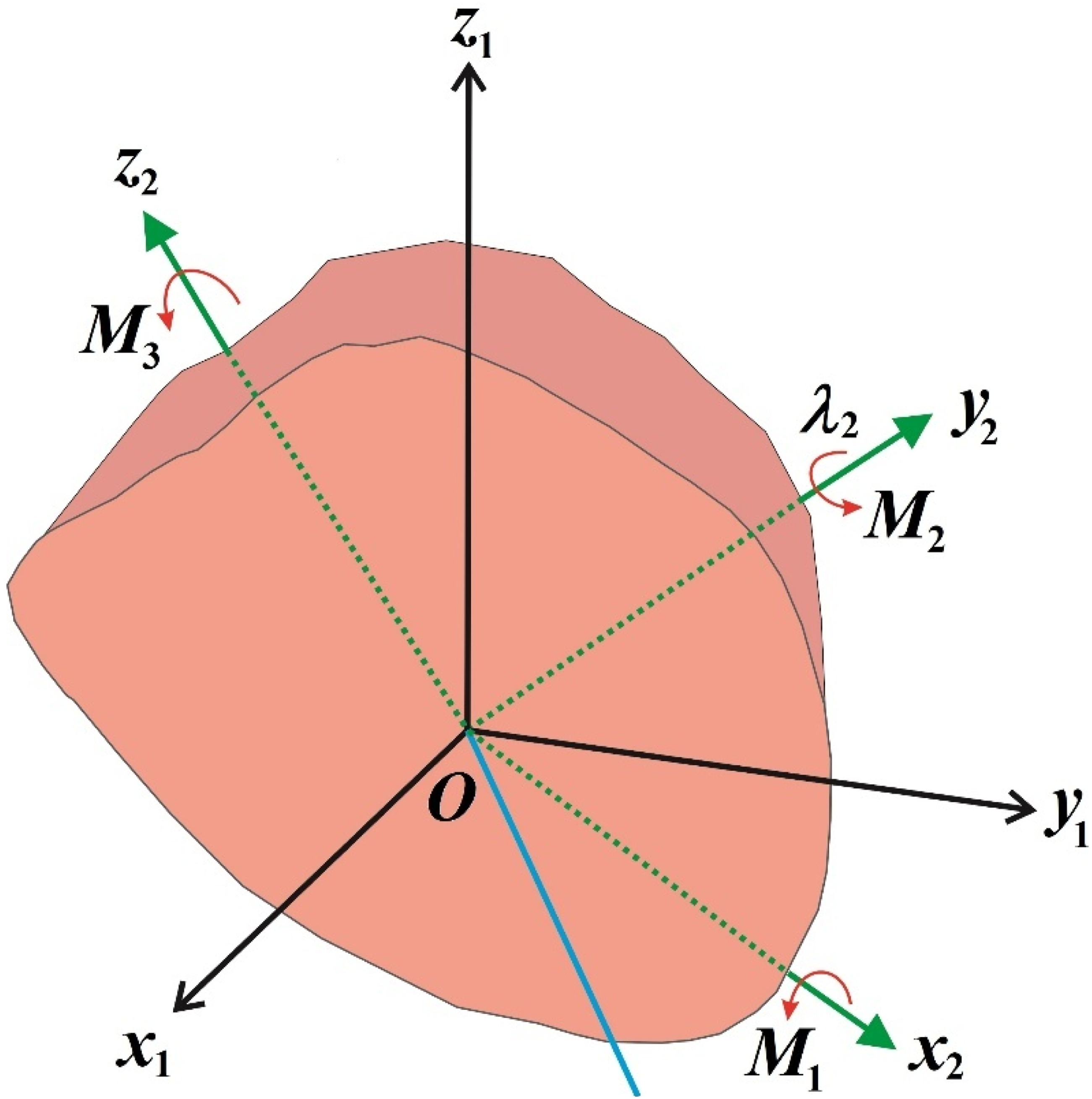
In this section, a detailed description of the problem has been presented. The presented model is an asymmetric RB rotating about a fixed point $O$ concerning two frames; one $O{x}_1{y}_1{z}_1$ is the inertial, while the other $O{x}_2{y}_2{z}_2$ is the rotational. The rotary motion of the RB is impacted by two torques. The first one is the GT which arises from a located rotating rotor on the intermediate axis, as $\underset{\_}{\lambda }=\left(0,{\lambda }_2,0\right)$ , where the first and third components of the GT along the major and minor axes are disregarded. The second one is the acting BCFTs $\underset{\_}{M}=\left(M_1,M_2,M_3\right)$ along the body’s principal axes $O{x}_2,O{y}_2,$ and $O{z}_2$ , respectively, see Figure 1.

Figure 1.

A simulated model for the RB’s motion.

Euler’s EOMs for the RB are given by^4,5

$\begin{array}{l}{D}_1{\dot{\omega }}_1=M_1-\left(D_3-D_2\right){\omega }_2{\omega }_3+{\lambda }_2{\omega }_3,\\ D_2{\dot{\omega }}_2=M_2-\left(D_1-D_3\right){\omega }_3{\omega }_1,\\ D_3{\dot{\omega }}_3=M_3-\left(D_2-D_1\right){\omega }_1{\omega }_2-{\lambda }_2{\omega }_1,\end{array}$

(1)

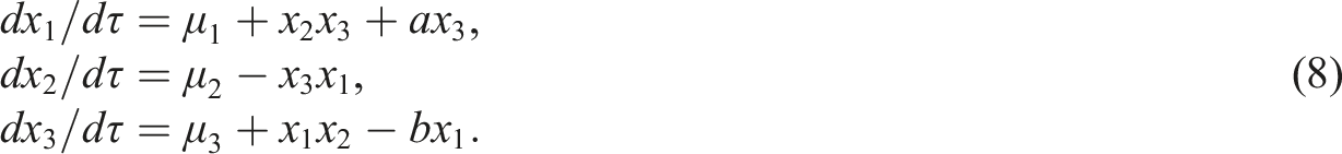
where the dots represent the differentiating concerning time $t$ , the RB’s angular velocities are denoted by $\underset{\_}{\omega }=\left({\omega }_1,{\omega }_2,{\omega }_3\right)$ and the BCFTs vector components are $\left(M_1,M_2,M_3\right)$ , while ${\lambda }_2$ is the second component of the GT vector $\underset{\_}{\lambda }$ which directed along $O{y}_2$ , where ${\lambda }_1={\lambda }_3=0$ . The principal inertia torques are denoted by $D=\left(D_1,D_2,D_3\right)$ as $D_1>D_2>D_3$ .

Considering the following new parameters

$\begin{array}{l}{k}_1=\left(D_2-D_3\right)/D_1, k_2=\left(D_1-D_3\right)/D_2, k_3=\left(D_1-D_2\right)/D_3,\\ u_j=M_j/D_j, k=k_1{k}_2{k}_3, T=\sqrt{k}\hspace{0.17em}t, {\mathrm{\Pi }}_j=u_j/\sqrt{k}\sqrt{k_j},\\ a={\lambda }_2/D_1{k}_1\sqrt{k_2}, b={\lambda }_2/D_3{k}_3\sqrt{k_2}, {\mathrm{\Omega }}_j={\omega }_j/\sqrt{k_j}, \left(j=1,2,3\right).\end{array}$

(2)

System (1) is transformed into

$\begin{array}{l}d{\mathrm{\Omega }}_1/dT={\mathrm{\Pi }}_1+{\mathrm{\Omega }}_2{\mathrm{\Omega }}_3+a{\mathrm{\Omega }}_3,\\ d{\mathrm{\Omega }}_2/dT={\mathrm{\Pi }}_2-{\mathrm{\Omega }}_3{\mathrm{\Omega }}_1,\\ d{\mathrm{\Omega }}_3/dT={\mathrm{\Pi }}_3+{\mathrm{\Omega }}_1{\mathrm{\Omega }}_2-b{\mathrm{\Omega }}_1,\end{array}$

(3)

where ${\mathrm{\Omega }}_j,{\mathrm{\Pi }}_j,$ and $T$ denote the NAVCs, BCFTs, and time, respectively. The EOMs at a steady state are

$\begin{array}{l}{X}_3\left(X_2+a\right)=-{\mathrm{\Pi }}_1,\\ X_3{X}_1={\mathrm{\Pi }}_2,\\ X_1\left(X_2-b\right)=-{\mathrm{\Pi }}_3,\end{array}$

(4)

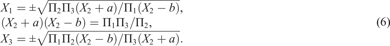
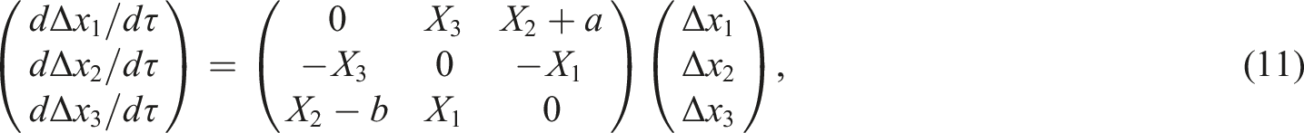
where the EP is represented by $\left(X_1,X_2,X_3\right).$ Hence

${X_1}^2{X_3}^2\left(X_2+a\right)\left(X_2-b\right)={\mathrm{\Pi }}_1{\mathrm{\Pi }}_2{\mathrm{\Pi }}_3.$

(5)

So that, if and only if ${\mathrm{\Pi }}_1{\mathrm{\Pi }}_2{\mathrm{\Pi }}_3\ge 0$ , the system will present eight EPs by knowing the value of ${\mathrm{\Pi }}_j$ as

$\begin{array}{l}{X}_1=\pm \sqrt{{\mathrm{\Pi }}_2{\mathrm{\Pi }}_3\left(X_2+a\right)/{\mathrm{\Pi }}_1\left(X_2-b\right)},\\ \left(X_2+a\right)\left(X_2-b\right)={\mathrm{\Pi }}_1{\mathrm{\Pi }}_3/{\mathrm{\Pi }}_2,\\ X_3=\pm \sqrt{{\mathrm{\Pi }}_1{\mathrm{\Pi }}_2\left(X_2-b\right)/{\mathrm{\Pi }}_3\left(X_2+a\right)}.\end{array}$

(6)

The dependence of system (1) on the values of the BCFTS $\left(M_1,M_2,M_3\right)$ is no longer satisfied, as a result of introducing the parameter $u=\sqrt{k_2{k}_3{u}_1^2+k_3{k}_1{u}_2^2+k_1{k}_2{u}_3^2}/k$ ⁴ and redefining ${\mathrm{\Omega }}_j,{\mathrm{\Pi }}_j,$ and $T$ as $x_j,{\mu }_j,$ and $\tau$ in the formulae

$\tau =\sqrt{k u}\hspace{0.17em}t, x_j={\omega }_j/\sqrt{u k_j}, {\mu }_j=u_j/u \sqrt{k}\sqrt{k_j}, \left(j=1,2,3\right),$

(7)

substituting (7) into (1), yields

$\begin{array}{l}d{x}_1/d\tau ={\mu }_1+x_2{x}_3+a{x}_3,\\ d{x}_2/d\tau ={\mu }_2-x_3{x}_1,\\ d{x}_3/d\tau ={\mu }_3+x_1{x}_2-b{x}_1.\end{array}$

(8)

Effectively utilizing system (7) implies

${\mu }_1^2+{\mu }_2^2+{\mu }_3^2=1.$

(9)

Introducing the perturbation state as ⁵

$\mathrm{\Delta } x_j=x_j-X_j.$

(10)

The linearized form of these EOMs is given by

$\left(\begin{array}{l}d\mathrm{\Delta }{x}_1/d\tau \\ d\mathrm{\Delta }{x}_2/d\tau \\ d\mathrm{\Delta }{x}_3/d\tau \end{array}\right)=\left(\begin{array}{ccc}0& X_3& X_2+a\\ -X_3& 0& -X_1\\ X_2-b& X_1& 0\end{array}\right)\left(\begin{array}{l}\mathrm{\Delta }{x}_1\\ \mathrm{\Delta }{x}_2\\ \mathrm{\Delta }{x}_3\end{array}\right),$

(11)

as the characteristic equation of system (11) is

${\xi }^3+\xi \left[X_1^2-\left(X_2+a\right)\left(X_2-b\right)+X_3^2\right]+X_1{X}_3\left(2X_2+a-b\right)=0.$

(12)

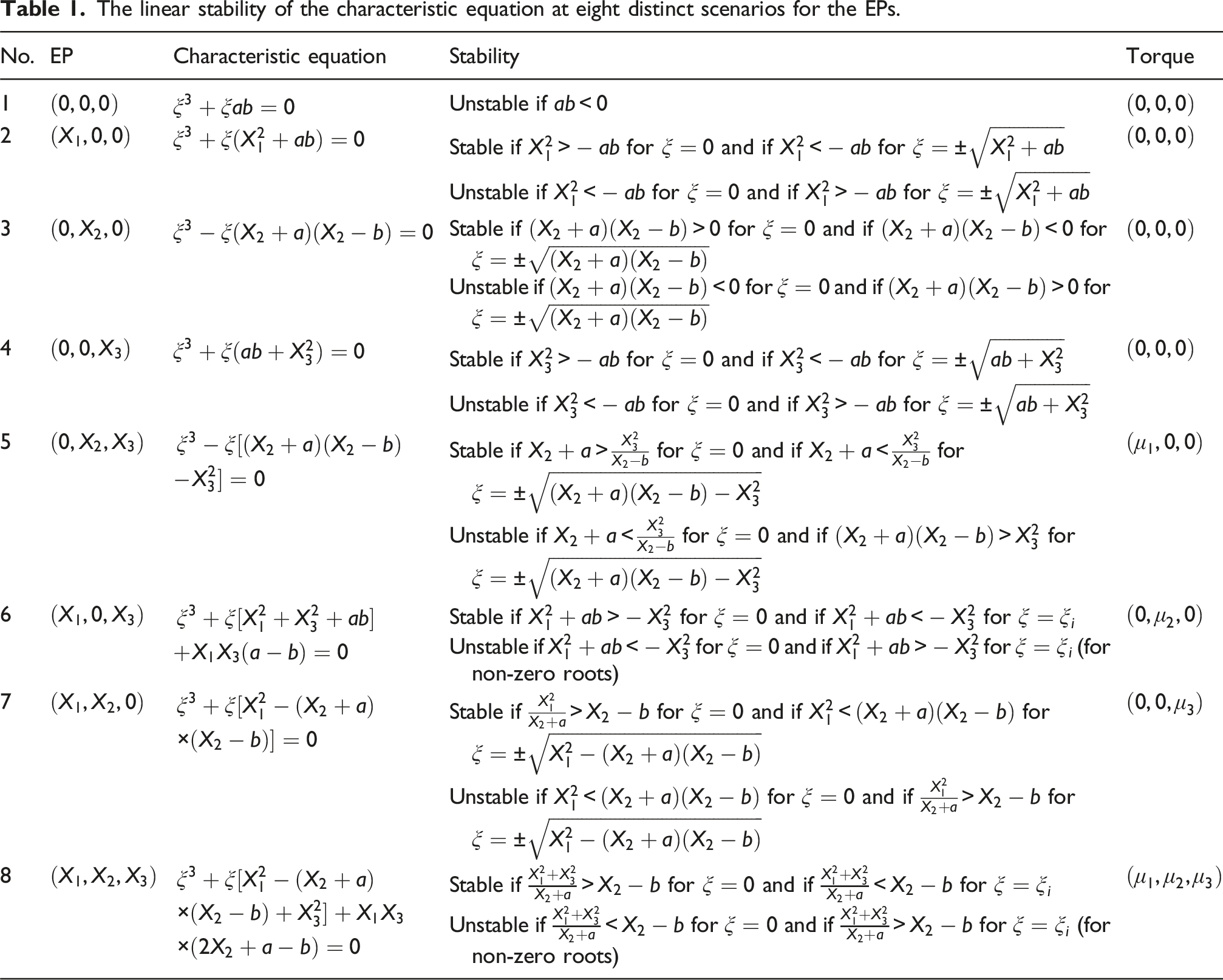
Table 1 provides the necessary conditions for the roots of the characteristic equation (12) to exist and be stable, as well as an exhaustive list of every conceivable pairing of BCFTs and EPs.

Table 1.

The linear stability of the characteristic equation at eight distinct scenarios for the EPs.

No.	EP	Characteristic equation	Stability	Torque
1	$\left(0,0,0\right)$	${\xi }^3+\xi ab=0$	Unstable if $ab<0$	$\left(0,0,0\right)$
2	$\left(X_1,0,0\right)$	${\xi }^3+\xi \left(X_1^2+ab\right)=0$	Stable if $X_1^2>-ab$ for $\xi =0$ and if $X_1^2<-ab$ for $\xi =\pm \sqrt{X_1^2+ab}$	$\left(0,0,0\right)$
			Unstable if $X_1^2<-ab$ for $\xi =0$ and if $X_1^2>-ab$ for $\xi =\pm \sqrt{X_1^2+ab}$
3	$\left(0,X_2,0\right)$	${\xi }^3-\xi \left(X_2+a\right)\left(X_2-b\right)=0$	Stable if $\left(X_2+a\right)\left(X_2-b\right)>0$ for $\xi =0$ and if $\left(X_2+a\right)\left(X_2-b\right)<0$ for $\xi =\pm \sqrt{\left(X_2+a\right)\left(X_2-b\right)}$	$\left(0,0,0\right)$
			Unstable if $\left(X_2+a\right)\left(X_2-b\right)<0$ for $\xi =0$ and if $\left(X_2+a\right)\left(X_2-b\right)>0$ for $\xi =\pm \sqrt{\left(X_2+a\right)\left(X_2-b\right)}$
4	$\left(0,0,X_3\right)$	${\xi }^3+\xi \left(ab+X_3^2\right)=0$	Stable if $X_3^2>-ab$ for $\xi =0$ and if $X_3^2<-ab$ for $\xi =\pm \sqrt{ab+X_3^2}$	$\left(0,0,0\right)$
			Unstable if $X_3^2<-ab$ for $\xi =0$ and if $X_3^2>-ab$ for $\xi =\pm \sqrt{ab+X_3^2}$
5	$\left(0,X_2,X_3\right)$	$\begin{array}{l}{\xi }^3-\xi [\left(X_2+a\right)\left(X_2-b\right)\\ -X_3^2]=0\end{array}$	Stable if $X_2+a>\frac{X_3^2}{X_2-b}$ for $\xi =0$ and if $X_2+a<\frac{X_3^2}{X_2-b}$ for $\xi =\pm \sqrt{\left(X_2+a\right)\left(X_2-b\right)-X_3^2}$	$\left({\mu }_1,0,0\right)$
			Unstable if $X_2+a<\frac{X_3^2}{X_2-b}$ for $\xi =0$ and if $\left(X_2+a\right)\left(X_2-b\right)>X_3^2$ for $\xi =\pm \sqrt{\left(X_2+a\right)\left(X_2-b\right)-X_3^2}$
6	$\left(X_1,0,X_3\right)$	$\begin{array}{l}{\xi }^3+\xi \left[X_1^2+X_3^2+ab\right]\\ +X_1{X}_3\left(a-b\right)=0\end{array}$	Stable if $X_1^2+ab>-X_3^2$ for $\xi =0$ and if $X_1^2+ab<-X_3^2$ for $\xi ={\xi }_i$	$\left(0,{\mu }_2,0\right)$
			Unstable if $X_1^2+ab<-X_3^2$ for $\xi =0$ and if $X_1^2+ab>-X_3^2$ for $\xi ={\xi }_i$ (for non-zero roots)
7	$\left(X_1,X_2,0\right)$	$\begin{array}{l}{\xi }^3+\xi [X_1^2-\left(X_2+a\right)\\ \times \left(X_2-b\right)]=0\end{array}$	Stable if $\frac{X_1^2}{X_2+a}>X_2-b$ for $\xi =0$ and if $X_1^2<\left(X_2+a\right)\left(X_2-b\right)$ for $\xi =\pm \sqrt{X_1^2-\left(X_2+a\right)\left(X_2-b\right)}$	$\left(0,0,{\mu }_3\right)$
			Unstable if $X_1^2<\left(X_2+a\right)\left(X_2-b\right)$ for $\xi =0$ and if $\frac{X_1^2}{X_2+a}>X_2-b$ for $\xi =\pm \sqrt{X_1^2-\left(X_2+a\right)\left(X_2-b\right)}$
8	$\left(X_1,X_2,X_3\right)$	$\begin{array}{l}{\xi }^3+\xi [X_1^2-\left(X_2+a\right)\\ \times \left(X_2-b\right)+X_3^2]+X_1{X}_3\\ \times \left(2X_2+a-b\right)=0\end{array}$	Stable if $\frac{X_1^2+X_3^2}{X_2+a}>X_2-b$ for $\xi =0$ and if $\frac{X_1^2+X_3^2}{X_2+a}<X_2-b$ for $\xi ={\xi }_i$	$\left({\mu }_1,{\mu }_2,{\mu }_3\right)$
			Unstable if $\frac{X_1^2+X_3^2}{X_2+a}<X_2-b$ for $\xi =0$ and if $\frac{X_1^2+X_3^2}{X_2+a}>X_2-b$ for $\xi ={\xi }_i$ (for non-zero roots)

Constant body torque in the major axis case

At $\left({\mu }_1,{\mu }_2,{\mu }_3\right)=\left(1,0,0\right),$ system (8) becomes

$\frac{d{x}_1}{d\tau }=1+x_2{x}_3+a{x}_3, \frac{d{x}_2}{d\tau }=-x_3{x}_1, \frac{d{x}_3}{d\tau }=x_1{x}_2-b{x}_1.$

(13)

In the absence of the time rate change of the scaled angular velocities in equation (13), it presents the equations of the EPs, where a hyperbola $X_3\left(X_2+a\right)=-1$ is formulated. Hence, the RB in such a case is stable at $\left|X_3\right|>1$ and unstable at $\left|X_2+a\right|>1$ . Introducing the variable ${\theta }_1$ ⁵ , and inserting it into the equation

${\theta }_1\left(\tau \right)=\underset{0}{\overset{\tau }{{\displaystyle \int }}}{x}_1\left({\alpha }_1\right)\hspace{0.17em}d{\alpha }_1\hspace{0.5em}\Rightarrow \hspace{1em}\frac{d{\theta }_1}{d\tau }=x_1\left(\tau \right),{\theta }_1\left(0\right)=0.$

(14)

Now, inserting ${\theta }_1$ into equation (13) gives

$\frac{d^2{\theta }_1}{d{\tau }^2}=1+x_2{x}_3+a{x}_3, \frac{d{x}_2}{d{\theta }_1}=-x_3, \frac{d{x}_3}{d{\theta }_1}=x_2-b.$

(15)

Solving the last two equations of (15) after differentiating concerning ${\theta }_1$ , yields two equations that imply the following solutions of $x_2$ and $x_3$ as

$x_2-b=A\hspace{0.17em}\cos \left({\theta }_1+{\eta }_1\right), x_3=A\hspace{0.17em}\sin \left({\theta }_1+{\eta }_1\right),$

(16)

where $A=\sqrt{{\left[x_2\left(0\right)-b\right]}^2+x_3^2\left(0\right)}$ and ${\eta }_1={\tan }^{-1}\left[x_3\left(0\right)/\left(x_2\left(0\right)-b\right)\right]$ as $\left|{\eta }_1\right|\le \pi$ . As a result, we have ${\left(x_2-b\right)}^2+x_3^2=A^2$ . This circle’s radius $A$ depends on the GT and the initial values of the first and second NAVCs and it is considered the motion first integral.

Substituting (16) into the first equation in (15) and using the substitution $\theta =2\left({\theta }_1+{\eta }_1\right)$ , yields

$\frac{d^2\theta }{d{\tau }^2}=A\left[A\hspace{0.17em}\sin \hspace{0.17em}\theta +2\left(a+b\right)\sin \frac{\theta }{2}\right]+2.$

(17)

For equilibrium’s angle ${\theta }^{*}$ without the presence of the GT, we approach that $\sin \hspace{0.17em}{\alpha }^{*}=-2/A^2$ . Hence, a new parameter is considered as $x=d\theta /d\tau$ , as a result, equation (17) is transformed into the $\left(\theta ,x\right)$ phase plane as

$\frac{dx}{d\tau }=A\left[A\hspace{0.17em}\sin \hspace{0.17em}\theta +2\left(a+b\right)\sin \left(\frac{\theta }{2}\right)\right]+2.$

(18)

Transforming the differentiation in (18) concerning $\theta$ then integrating the resulting equation gets

$\frac{x^2}{2}+A^2\hspace{0.17em}\cos \hspace{0.17em}\theta +4A\left(a+b\right)\cos \left(\frac{\theta }{2}\right)-2\theta =E_1,$

(19)

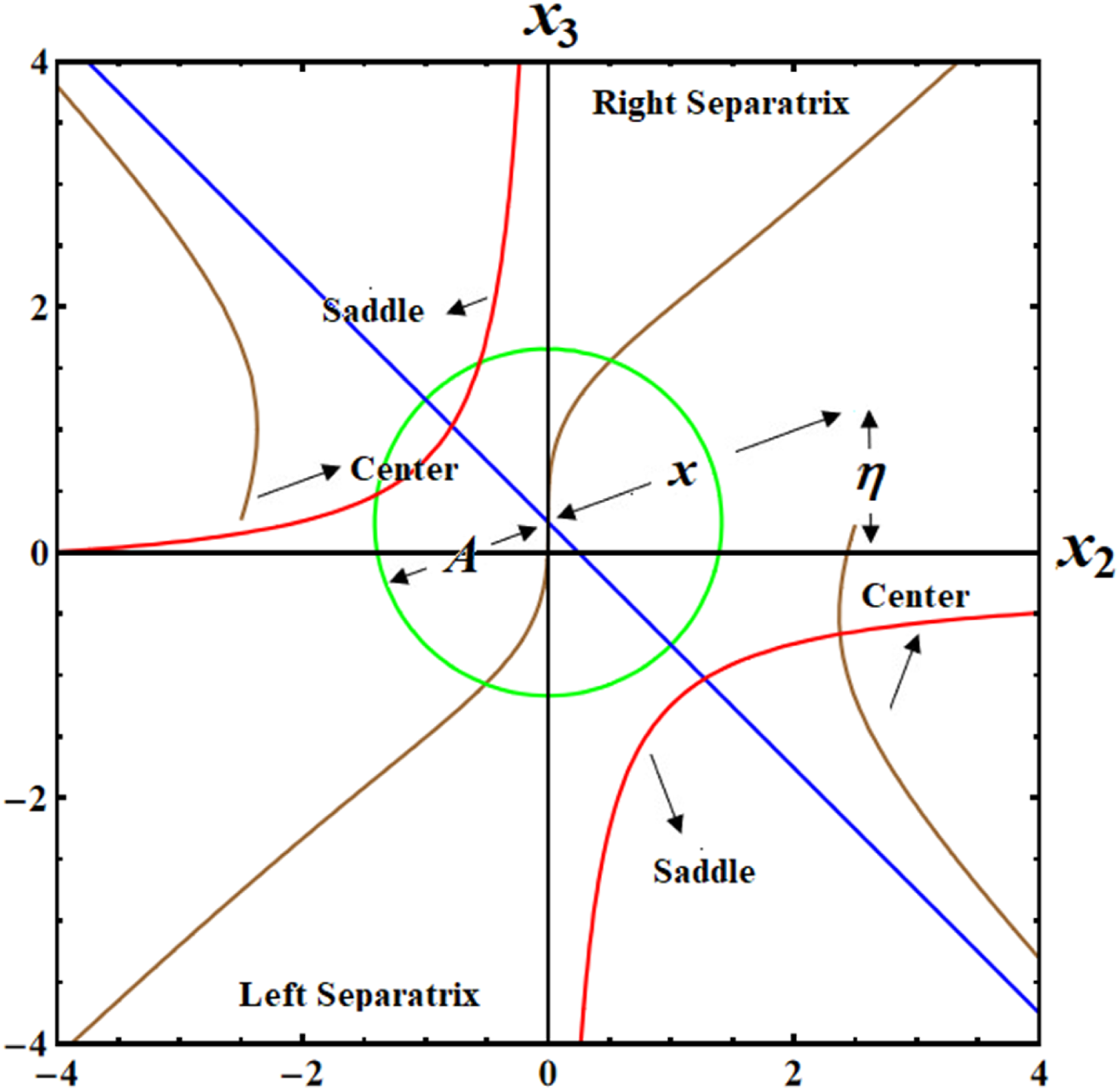
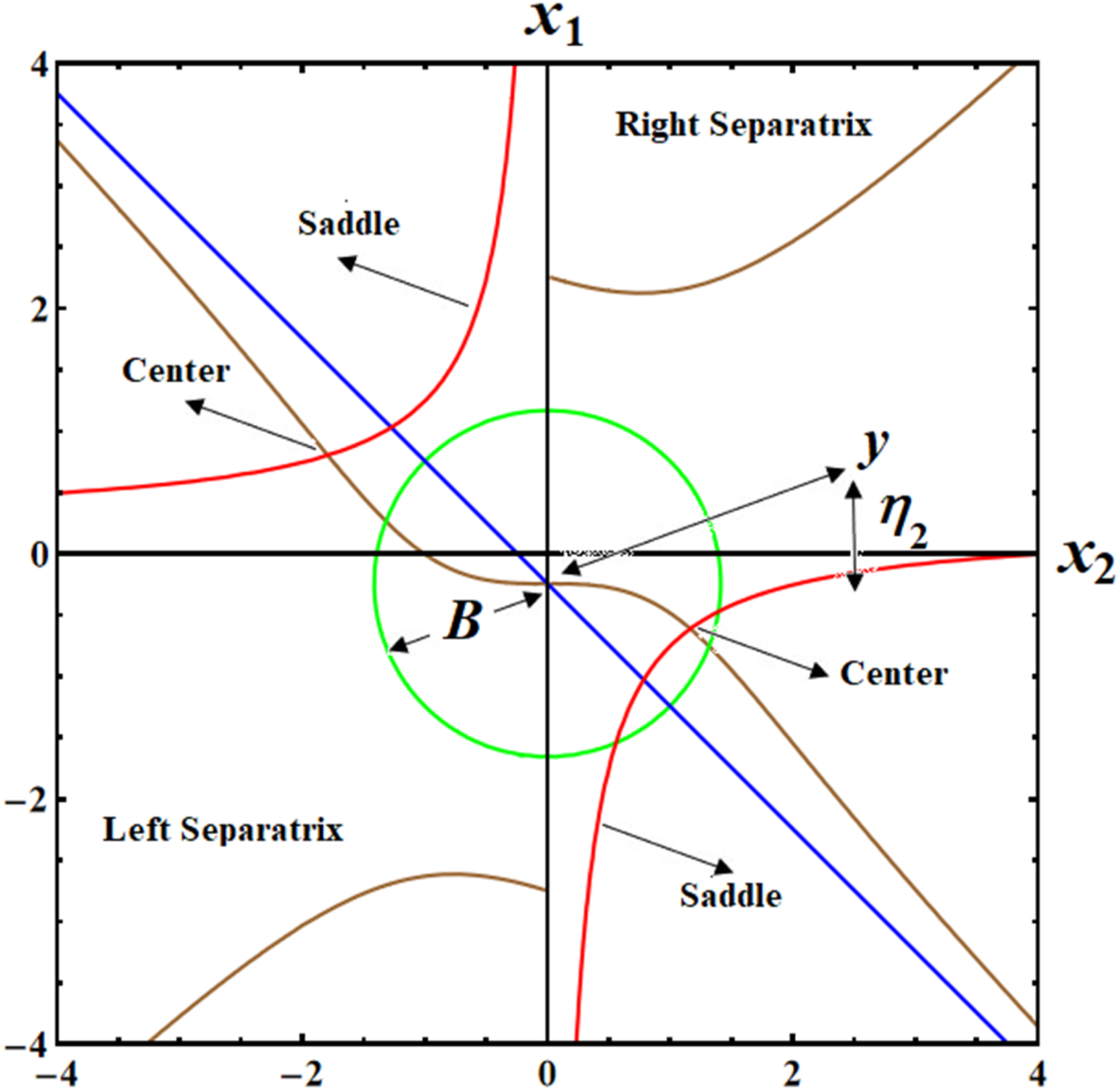
as the energy constant $E_1$ is the motion second integral. Equation (19), when applied to $E_1$ , allows us to draw contour plots on the plane $\left(\theta ,x\right)$ . As shown in Figure 2, the axis of the phase plane is periodically positioned along an infinite number of stable (centers ) and unstable (saddles $\circ$ ) EPs.

Figure 2.

The scaled angular velocity paths at constant torque along the major axis at $x\left(0\right)=\left(1.5,3,0.1\right)$ , $D=\left(2000,1500,1000\right)\text{kg}.{\mathrm{m}}^2$ , and ${\lambda }_2=100\text{kg}.{\mathrm{m}}^2.{\mathrm{s}}^{-1}$ .

For a SP ${\theta }_{\mathrm{s}}$ , the energy constant $E_{1\mathrm{s}}$ takes the form as

$E_{1\mathrm{s}}=A\left[A\hspace{0.17em}\cos \hspace{0.17em}{\theta }_{\mathrm{s}}+4\left(a+b\right)\cos \frac{{\theta }_{\mathrm{s}}}{2}\right]-2{\theta }_{\mathrm{s}}.$

(20)

Therefore

$\frac{x^2}{2}+A\left[A\hspace{0.17em}\cos \hspace{0.17em}\theta +4\left(a+b\right)\cos \frac{\theta }{2}\right]-2\theta =E_{1\mathrm{s}}.$

(21)

Substituting from equation (20) into equation (21) implies

$x=\pm \sqrt{2}A\sqrt{\left(\cos \hspace{0.17em}{\theta }_s-\cos \hspace{0.17em}\theta \right)+4\left(a+b\right)\{\left[\cos \frac{{\theta }_{\mathrm{s}}}{2}-\cos \frac{\theta }{2}\right]/A\}+\left({\theta }_{\mathrm{s}}-\theta \right)\sin \hspace{0.17em}{\theta }_{\mathrm{s}}}\hspace{0.17em}.$

(22)

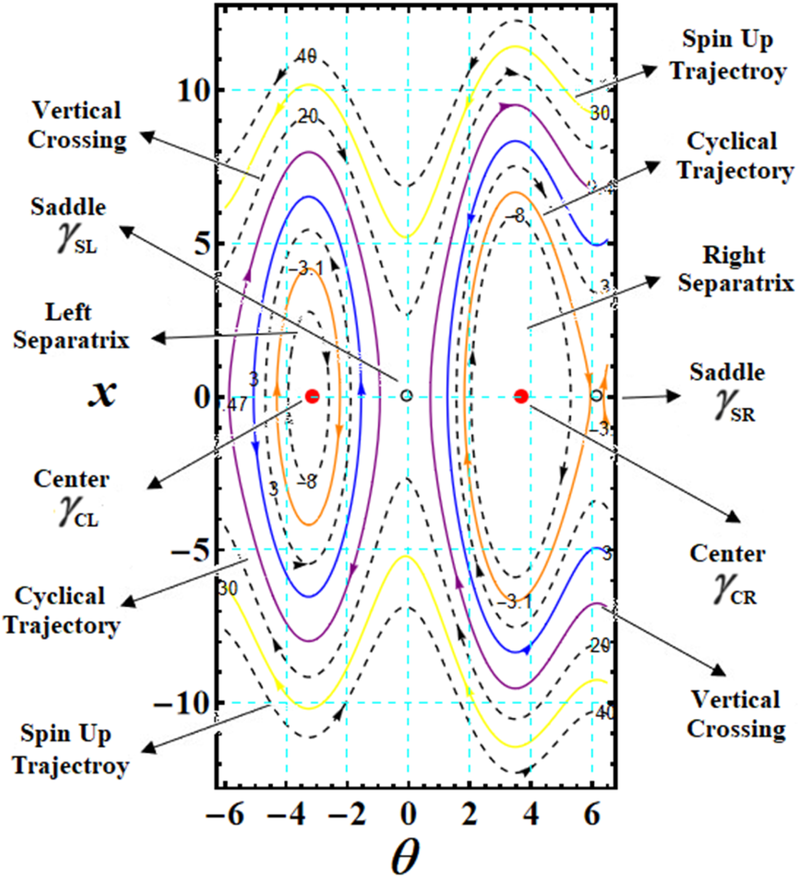
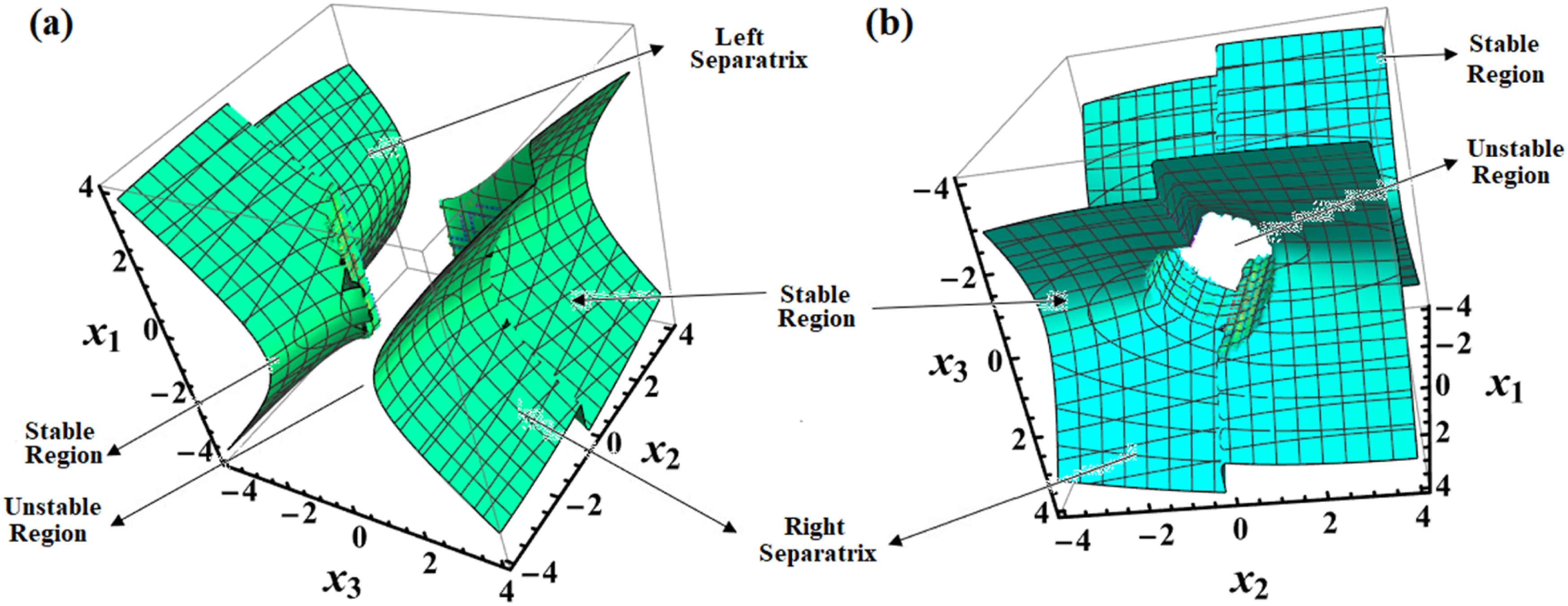
Recalling that $\theta \left(0\right)=2{\eta }_1$ and $\left|{\eta }_1\right|\le \pi$ . In terms of stability analysis, there are only two significant SS to consider: the left separatrix (LS), which passes through the left SP at ${\gamma }_{\text{SL}}$ before encircling the left CP at ${\gamma }_{\text{CL}}$ , and the right separatrix (RS), which passes through the right SP at ${\gamma }_{\text{SR}}$ before encircling the right CP at ${\gamma }_{\text{CR}}$ . In Figure 3, the RS and LS are shown along with the connected CPs and SPs. The diagram also demonstrates the spin-up, cyclical, and vertical crossing (VC) paths occurring during the activity.

Figure 3.

The paths of the LS and RS at stationary torque on the major axis at the same values as Figure 2.

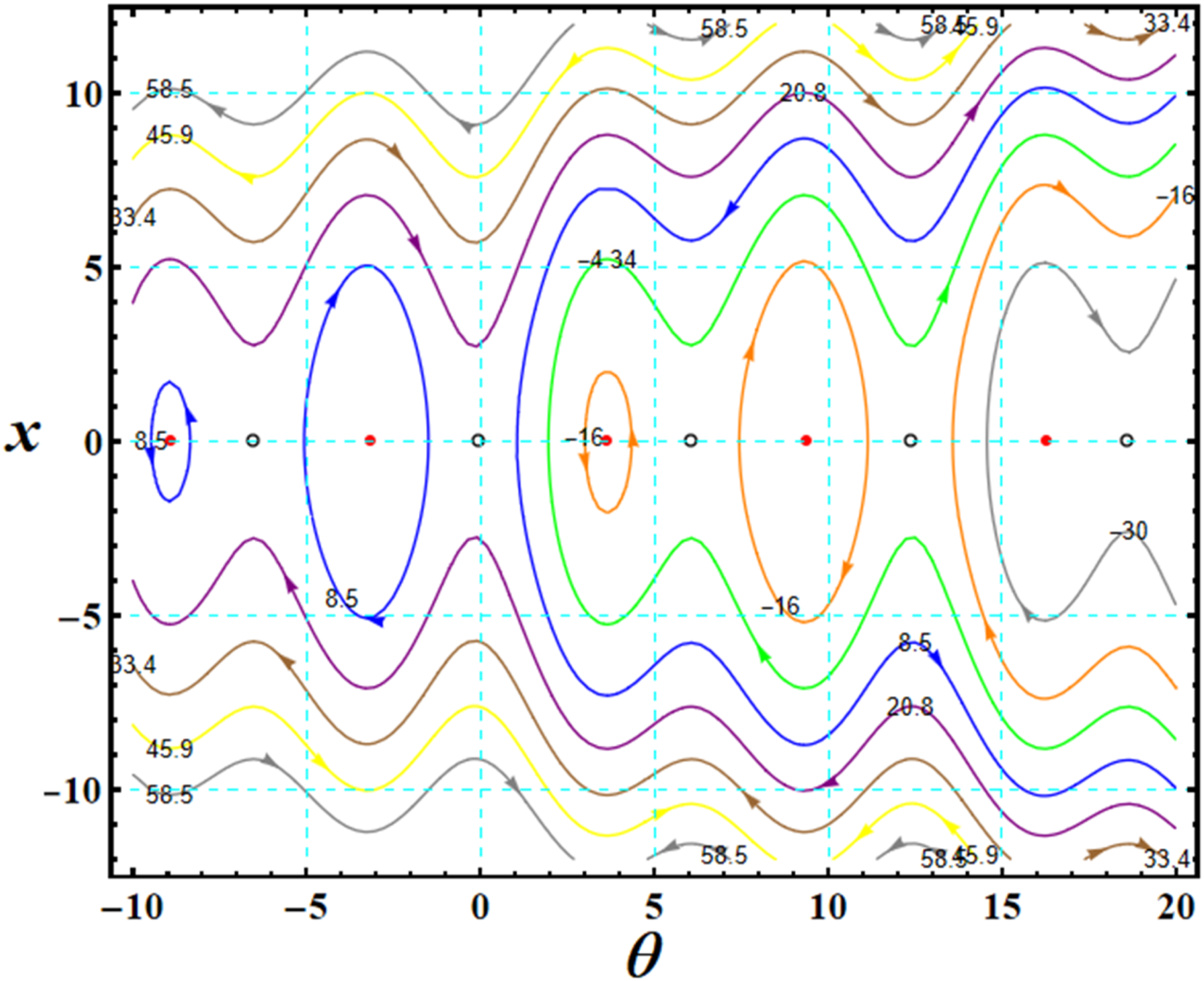
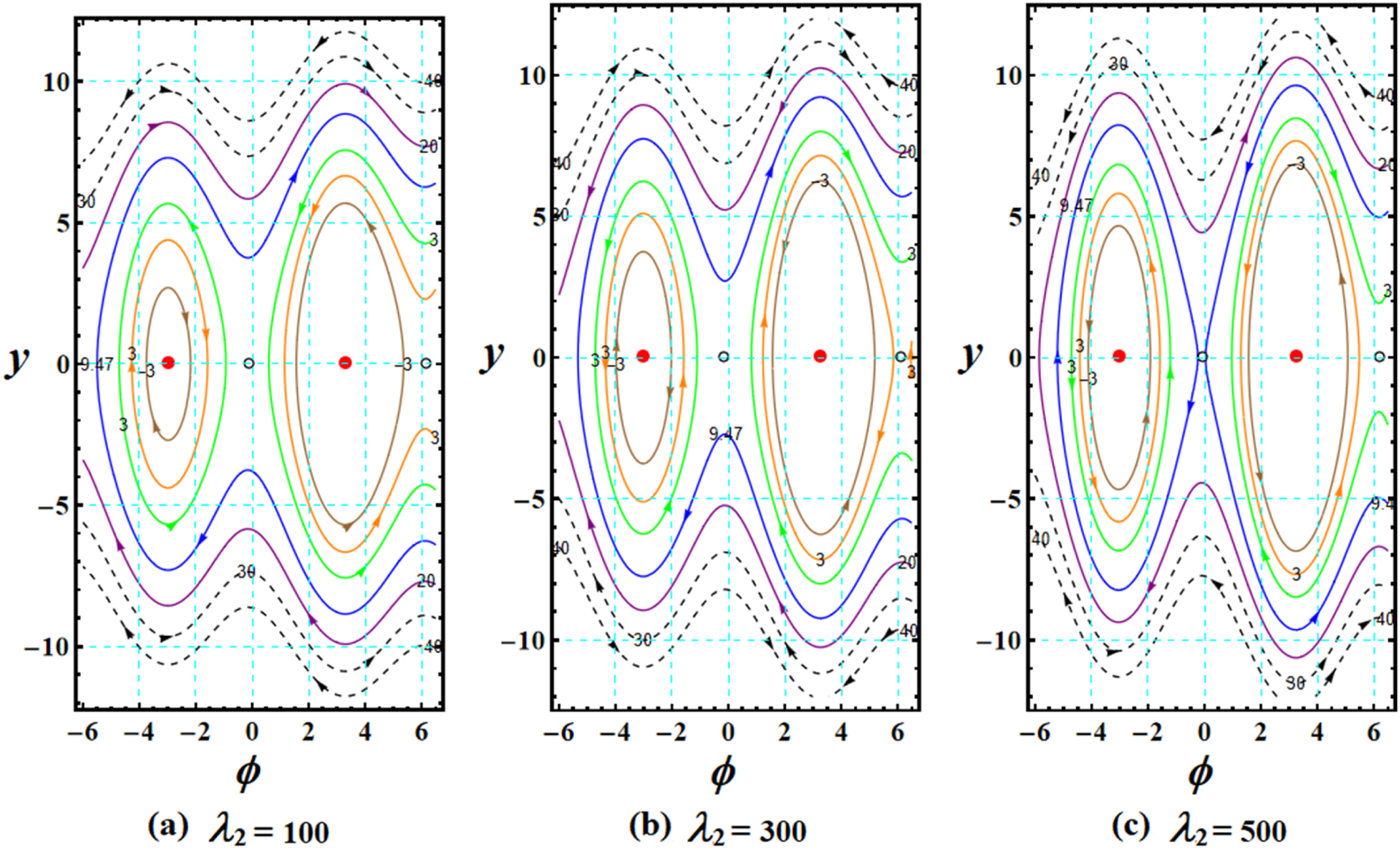
The influence of distinct values of the GT on the scaled angular velocity paths is shown in Figure 4. In portion (a) of the figure at ${\lambda }_2=100,$ the graphical representation shows the LS and RS as the cyclical paths increase in the LS more than the RS around the CPs; ${\gamma }_{\text{CL}}=\left(-3.2,0\right)$ and ${\gamma }_{\text{CR}}=\left(3.7,0\right),$ while VC and spin-up paths make a half-cyclic path around the CPs while spin-up occurs around the SPs; ${\gamma }_{\text{SL}}=\left(-0.1,0\right)$ and ${\gamma }_{\text{SR}}=\left(6.1,0\right).$

Figure 4.

The impact of the GT on the LS and RS at ${\lambda }_2=\left(100,300,500\right)\text{kg}.{\mathrm{m}}^2.{\mathrm{s}}^{-1}$ .

Increasing the GT value into ${\lambda }_2=300$ implies a decrease in the cyclical paths in the LS and vanishing in the RS, while increasing the VC, and spin-up paths in the LS and RS also increases the amplitude of the paths in the RS and decreases in the LS. Also, a change is occurring in the positions of the CPs and the SPs as ${\gamma }_{\text{CL}}=\left(-3.8,0\right),{\gamma }_{\text{CR}}=\left(3.9,0\right),{\gamma }_{\text{SL}}=\left(-0.5,0\right),$ and ${\gamma }_{\text{SR}}=\left(6,0\right).$

A greater increase in the GT as it equals ${\lambda }_2=500$ ends the existence of the cyclic paths and converges all paths in both RS and LS into VCs or spinning up trajectories which increases the values of the scaled angular velocities in the positive direction. Again, changing the positions of the CPs and SPs into ${\gamma }_{\text{CL}}=\left(-4.2,0\right),{\gamma }_{\text{CR}}=\left(4.3,0\right),{\gamma }_{\text{SL}}=\left(0,0\right),$ and ${\gamma }_{\text{SR}}=\left(5.9,0\right)$ .

Taking into consideration that

$x=2x_1, \cos \hspace{0.17em}\theta =\frac{{\left(x_2-b\right)}^2-x_3^2}{A^2}, \alpha =2\hspace{0.17em}{\tan }^{-1}\frac{x_3}{x_2-b},$

(23)

substituting from (23) into (21), implies

$2x_1^2-x_3^2+{\left(x_2-b\right)}^2+4\left(a+b\right)\left(x_2-b\right)-4\hspace{0.17em}{\tan }^{-1}\frac{x_3}{x_2-b}=E_1.$

(24)

Taking into consideration that $\cos \hspace{0.17em}{\theta }_{\mathrm{s}}=\frac{\sqrt{\left(A^4-4\right)}}{A^2}$ and $\cos \frac{{\theta }_{\mathrm{s}}}{2}=\pm \sqrt{\frac{1+\cos \hspace{0.17em}{\alpha }_{\mathrm{s}}}{2}}$ , yields

$\begin{array}{l}2x_1^2-x_3^2+{\left(x_2-b\right)}^2+4\left(a+b\right)\left(x_2-b\right)-\sqrt{{\left[{\left(x_2-b\right)}^2+x_2^2\right]}^2-4}-4\hspace{0.17em}{\tan }^{-1}\frac{x_3}{x_2-b}\\ -2\hspace{0.17em}{\sin }^{-1}\frac{2}{{\left(x_2-b\right)}^2+x_3^2}\mp \frac{4\left(a+b\right)}{\sqrt{2}}\sqrt{x_3^2+{\left(x_2-b\right)}^2+\sqrt{{\left[{\left(x_2-b\right)}^2+x_3^2\right]}^2-4}}=0.\end{array}$

(25)

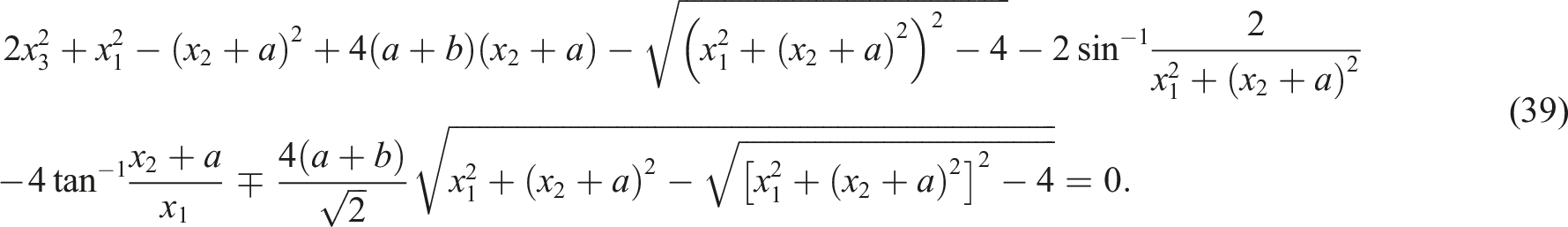
In Figure 5, the LS and RS surfaces divide the $\left(x_1,x_2,x_3\right)$ phase space. These surfaces create three infinite areas within the $\left(x_1,x_2,x_3\right)$ space: two stable areas and one unstable area. Any motion initiated within one of these areas is expected to remain confined to that region. Motion starting in a stable region will result in a closed trajectory rotating around its center, while motion starting in an unstable region will lead to a spin-up maneuver. For initial conditions inside the unstable area, the NAVCs $\left(x_1,x_2,x_3\right)$ on the $\left(x_2,x_3\right)$ plane forms a full complete circle, while for initial conditions in a stable area, it forms a partial circle. Therefore, this circle’s radius $A$ can change, leading to either stable or unstable motion.

Figure 5.

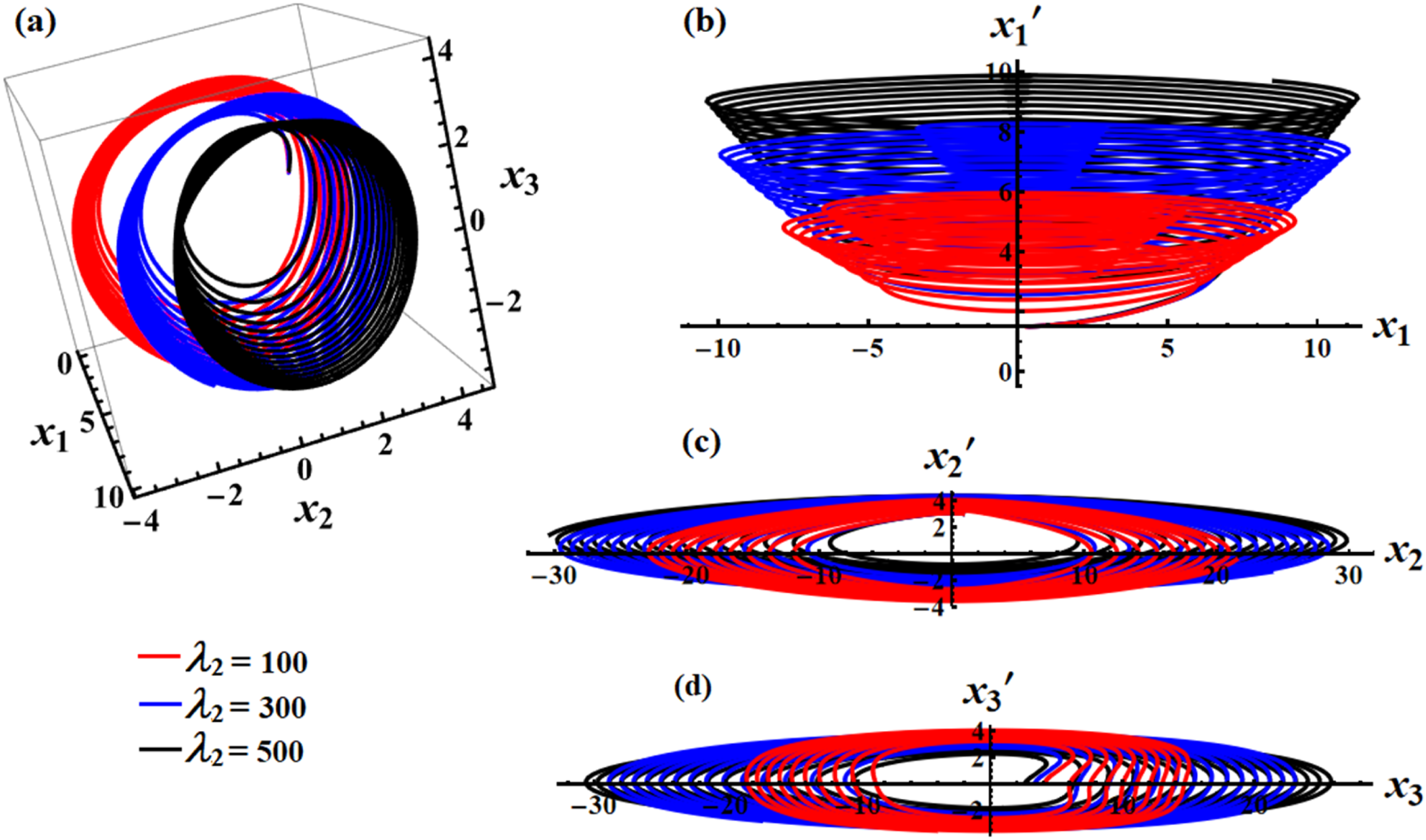
The 3D graphs for RS and LS at stationary torque directed on the major axis at ${\lambda }_2=100\text{kg}.{\mathrm{m}}^2.{\mathrm{s}}^{-1}$ .

At an initial value $x\left(0\right)=\left(1.5,3,0.1\right)$ and at a principal inertia’s moment $D=\left(2000,1500,1000\right)\text{kg}.{\mathrm{m}}^2$ , Figure 6 gives a simulation for the contour plots of some achieved SS at ${\lambda }_2=100\text{kg}.{\mathrm{m}}^2.{\mathrm{s}}^{-1}$ . These SS are $x_3\left(x_2+a\right)=-1,x_3+x_2-b=0,{\left(x_2-b\right)}^2-x_3^2+4\left(a+b\right)\left(x_2-b\right)-4\hspace{0.17em}{\tan }^{-1}\left[x_3/\left(x_2-b\right)\right]=0,$ and $\left[x_3^2+{\left(x_2-b\right)}^2\right]-4=0$ . The positions where the CP, SP, and VC points intersect with the RS and LS in Figure 2 correspond to the positions, in which a circle $A$ intersects with the CP, SP, and VC curves in Figure 6.

Figure 6.

The RS and LS surfaces at stationary torque along the major axis.

To solve the transcendental equations given by (22), it is necessary to determine where the two SS intersect with the $\left(x_2,x_3\right)$ plane

$\cos \hspace{0.17em}{\theta }_{\mathrm{s}}-\cos \hspace{0.17em}\theta +4\left(a+b\right)\left\{\left[\cos \frac{{\theta }_{\mathrm{s}}}{2}-\cos \frac{\theta }{2}\right]/F\right\}+\left({\theta }_{\mathrm{s}}-\theta \right)\sin \hspace{0.17em}{\theta }_{\mathrm{s}}=0\hspace{0.17em}.$

(26)

Assuming that $\theta ={\theta }_{\mathrm{s}}$ is a solution of (17), which leads to

$\sin \hspace{0.17em}{\theta }_s=\sin \hspace{0.17em}\theta =\frac{2\hspace{0.17em}\tan \left(\theta /2\right)}{1+{\tan }^2\left(\theta /2\right)}=\frac{2x_3\left(x_2-b\right)}{x_3^2+{\left(x_2-b\right)}^2}.$

(27)

A detailed representation of the maximum and minimum values of the NAVCs is approached (see Appendix A).

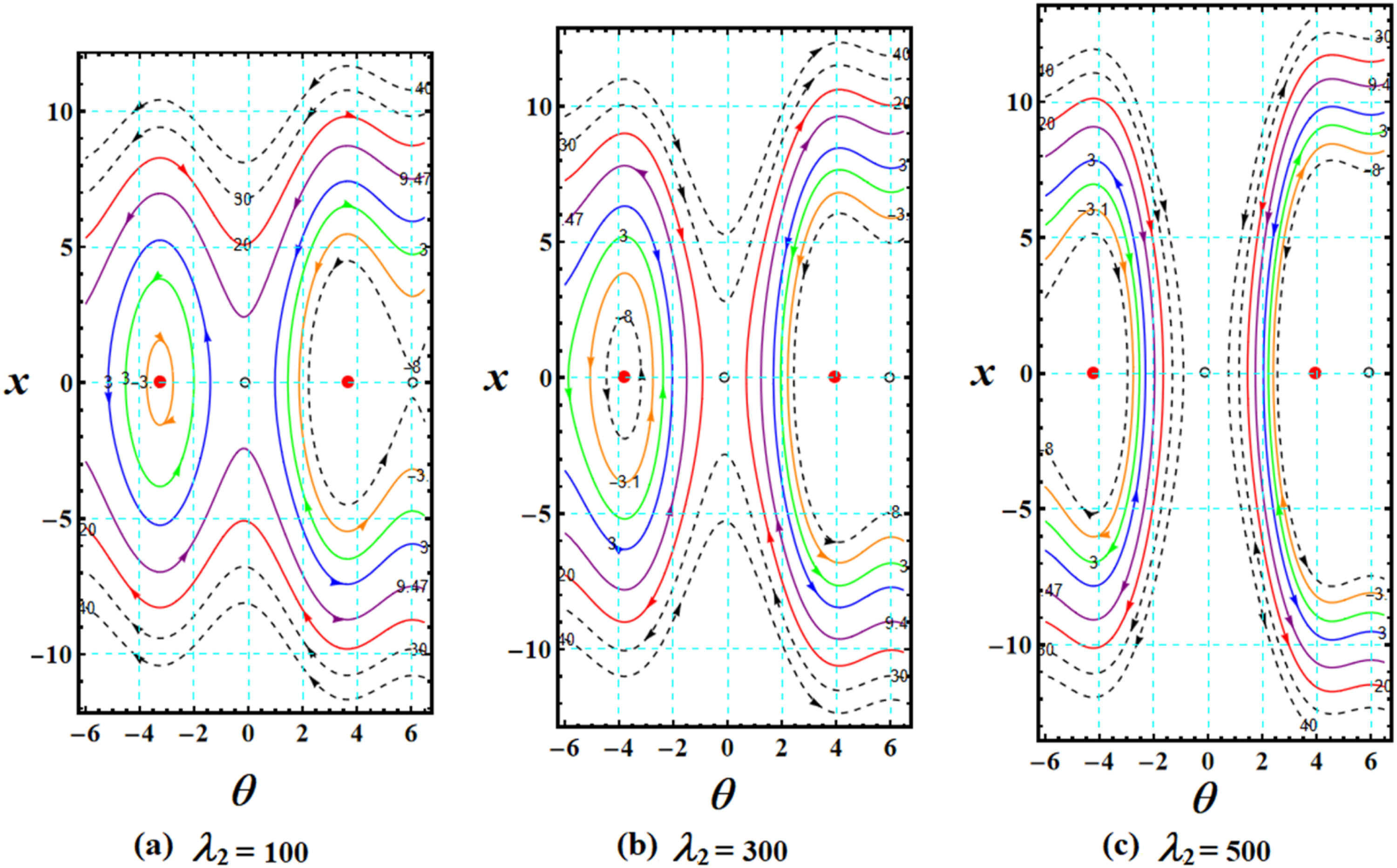
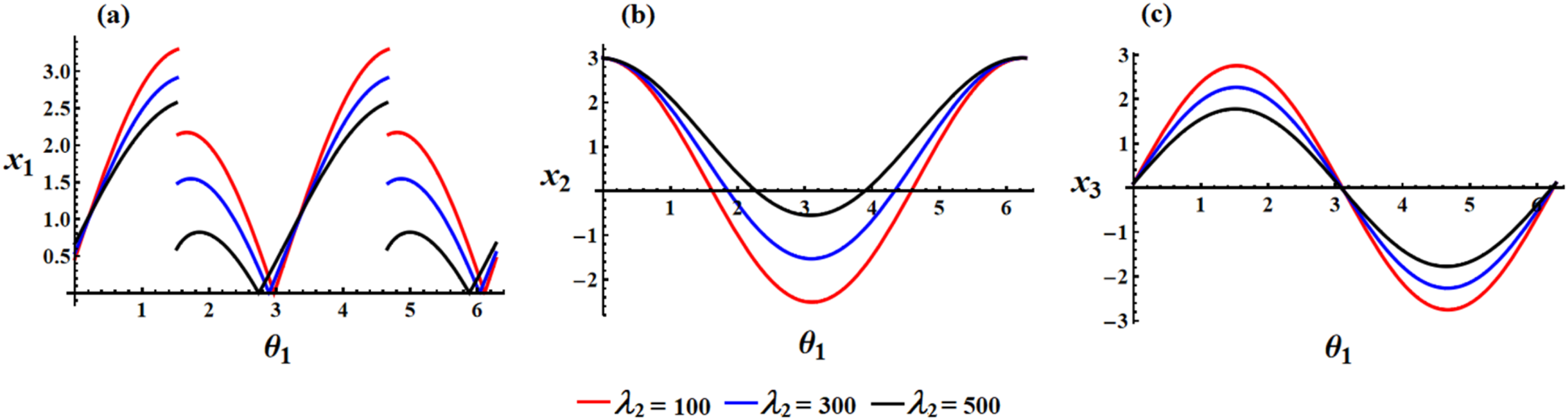
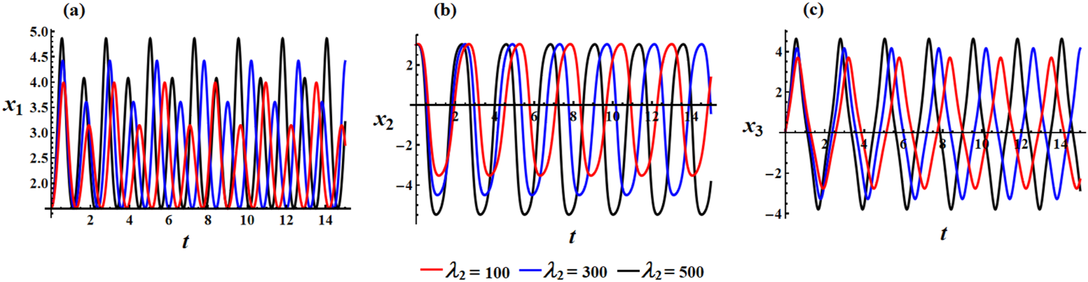
Figure 7 shows a simulation for the solutions in equations (16) and (25) of the NAVCs $x_1$ , $x_2$ , and $x_3$ during the period ${\theta }_1\in \left[0,2\pi \right]$ as the GT’s value varies with ${\lambda }_2=\left(100,300,500\right)\text{kg}.{\mathrm{m}}^2.{\mathrm{s}}^{-1}$ . The graph in portion (a) shows the biggest amplitudes ${\lambda }_2=100\text{kg}.{\mathrm{m}}^2.{\mathrm{s}}^{-1}$ . This implies that when the system rotates, $x_1$ will reach the largest maximum values, indicating a more dynamic and unconstrained angular motion. The curve’s periodicity indicates oscillatory behavior, in which the NAVC $x_1$ cycles symmetrically up and down.

Figure 7.

The GT influence on the NAVCs’ solution at stationary torque directed on the major axis.

The amplitude of oscillations decreases when ${\lambda }_2=300\text{kg}.{\mathrm{m}}^2.{\mathrm{s}}^{-1}$ , indicating greater constraint on $x_1$ . This implies that the motion is less extreme than the red curve because the growing gyrostatic effect dampens $x_1$ . The NAVC $x_1$ is further limited for the highest GT ${\lambda }_2=500\text{kg}.{\mathrm{m}}^2.{\mathrm{s}}^{-1}$ , yielding the least amplitude. The strongest limiting or damping impact of the GT on $x_1$ is indicated by the black curve. This proves that when the GT rises, the rotational motion will become more regulated or controlled. Repeated parabolic-like arcs can be seen on the graph; each cycle resembles a rise and decrease in $x_1$ .

This observation implies that when ${\theta }_1$ grows, $x_1$ ascends, then drops back toward zero, and the cycle repeats. The system’s periodic behavior indicates that it accelerates and decelerates repeatedly, perhaps as a result of the GT and other external forces acting on the system. This plot can be understood as illustrating how the GT dampens the system’s rotational dynamics. The system can reach greater NAVC $x_1$ for lower values of GT, which suggests more chaotic or unrestricted rotational motion. The system becomes more stable as GT rises, which means that $x_1$ is less variable and the system responds more predictably. This would be in line with systems where larger stabilization forces acting on the system cause a higher GT to result in decreased $x_1$ amplitudes.

In portion (b), according to the graph, $x_2$ behaves periodically with regard to ${\theta }_1$ , generally following a sinusoidal pattern with alternating peaks and troughs, just like $x_1$ did in earlier graphs. As the GT increases, the oscillations’ amplitude decreases, indicating a damping effect on $x_2$ . Whereas the biggest value (500) keeps $x_2$ more confined, a smaller GT (100) causes larger excursions in $x_2$ . The curve’s shape indicates that the system gets more stable, and the rotational motion becomes less unpredictable at higher values of GT. This is due to the fact that the GT lessens the size of $x_2$ variations by aiding in the control of the rotational dynamics. The graphs show how the RB’s rotational motion is dampened by the GT. The system is more dynamic, and it has more freedom in NAVCs like $x_2$ for smaller values of GT. The rotating motion gets more stable and regulated as GT grows, which lowers the oscillations’ amplitude in $x_2$ .

In portion (c), $x_3$ exhibits the biggest oscillations for ${\lambda }_2=100\text{kg}.{\mathrm{m}}^2.{\mathrm{s}}^{-1}$ , indicating that the system goes through substantial $x_3$ -fluctuations. Rapid variations in rotational speed across the interval are shown by the curve’s reaching both positive and negative peaks. When the GT is relatively low, the red curve exhibits the widest amplitude, indicating that the $x_3$ is more dynamic and has a higher DOF. Compared to the red curve, $x_3$ shows less oscillations for ${\lambda }_2=300\text{kg}.{\mathrm{m}}^2.{\mathrm{s}}^{-1}$ . As GT grows, the amplitude drops, suggesting that $x_3$ is becoming more restricted. Although the peaks are less prominent, the behavior is still periodic, indicating a dampened angular motion. The oscillations are further suppressed, with the least amplitude of the three curves, with ${\lambda }_2=500\text{kg}.{\mathrm{m}}^2.{\mathrm{s}}^{-1}$ . In contrast to lower GT values, these outcomes suggest that the system is strongly stable and that $x_3$ changes more gradually.

Figure 7(c) indicates that $x_3$ is significantly regulated by the GT. The system becomes more stable and $x_3$ is less susceptible to abrupt changes as the GT rises. The NAVC is more dynamic and fluctuates significantly in systems with a modest GT. Nevertheless, the system becomes more rotationally stable as the GT rises, as shown by the smaller $x_3$ -oscillations.

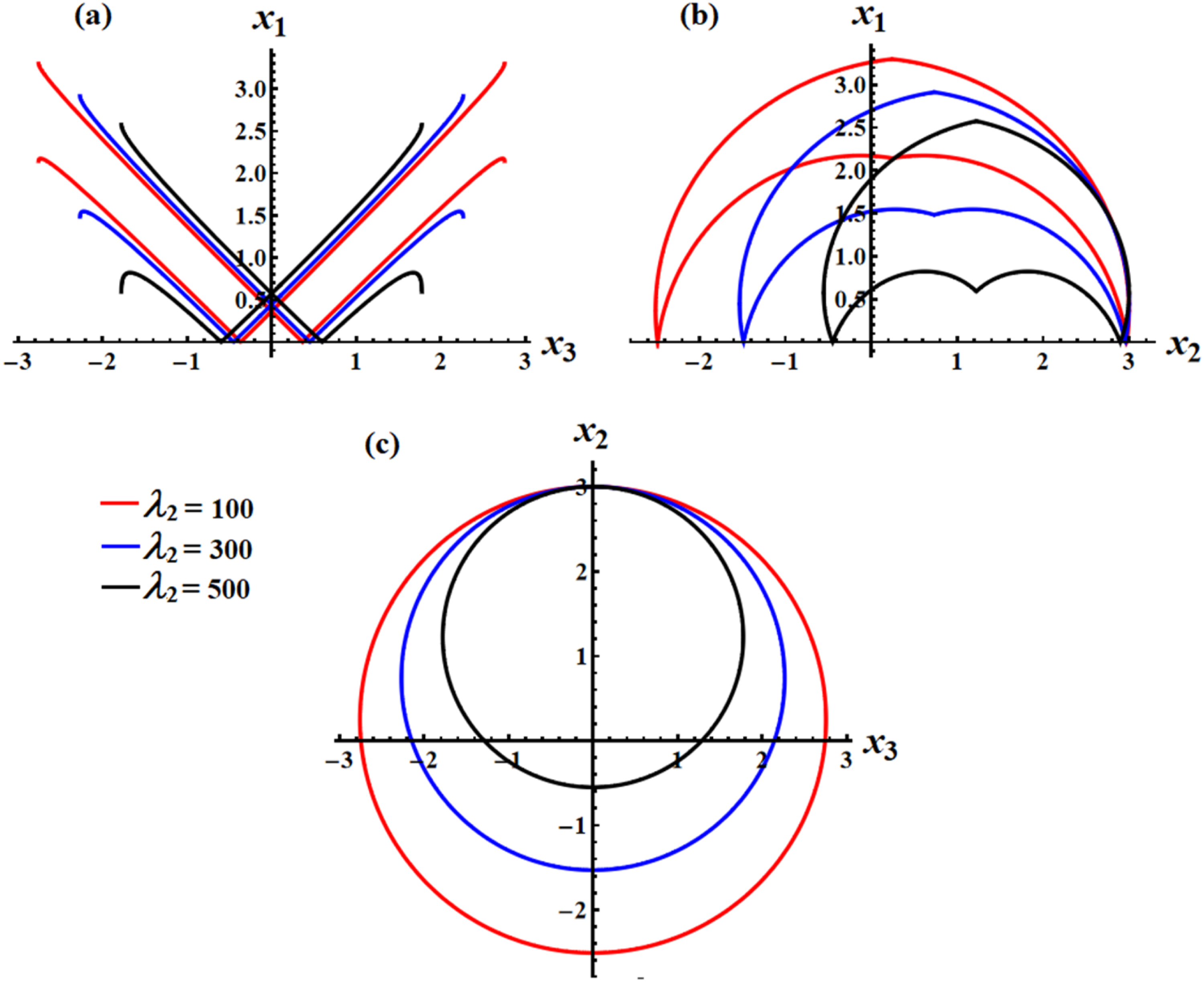
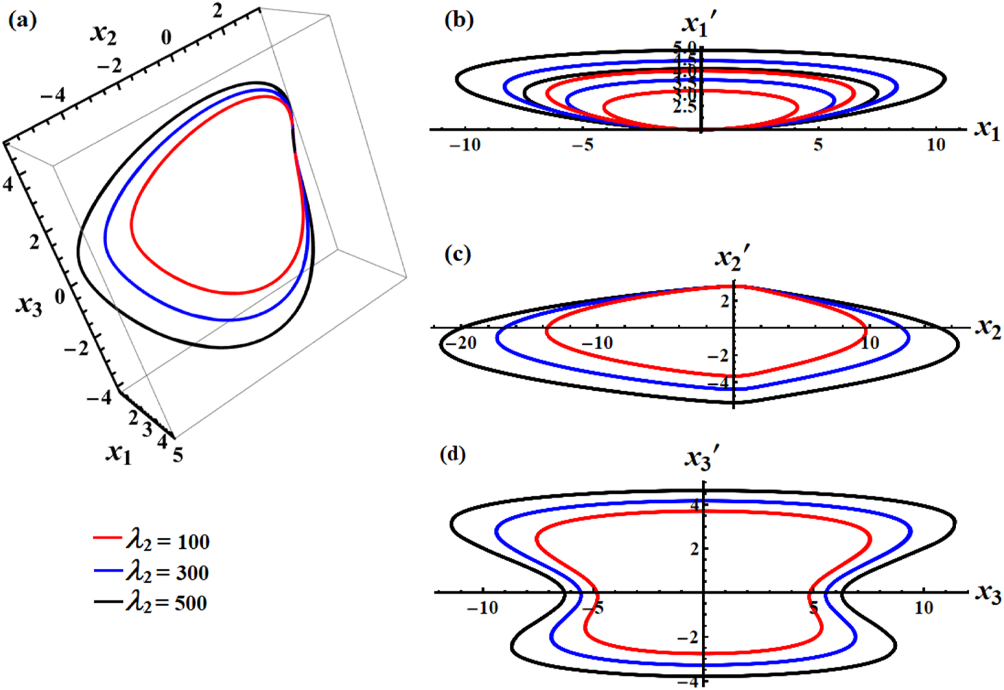
Figure 8 graphs a simulation for the relationship between the NAVCs $x_1$ , $x_2$ , and $x_3$ through the interval ${\theta }_1\in \left[0,2\pi \right]$ as the GT value varies with ${\lambda }_2=\left(100,300,500\right)\text{kg}.{\mathrm{m}}^2.{\mathrm{s}}^{-1}$ . The red curve in Figure 8(a) is consistent with ${\lambda }_2=100\text{kg}.{\mathrm{m}}^2.{\mathrm{s}}^{-1}$ , indicating a more symmetrical and dispersed distribution of $x_1$ compared to $x_3$ . Because of the wider curve, there are more NAVCs in relation to higher GT. The blue curve corresponds to ${\lambda }_2=300\text{kg}.{\mathrm{m}}^2.{\mathrm{s}}^{-1}$ and displays a less extreme spread than the red curve, with some constraints on the NAVCs. The relationship between $x_1$ and $x_3$ is steeper on the curve, indicating that as the GT grows, the system becomes less dynamic. The black curve has an even narrower path at ${\lambda }_2=500\text{kg}.{\mathrm{m}}^2.{\mathrm{s}}^{-1}$ , suggesting that the NAVCs are more strongly correlated at this high GT value, with smaller ranges of $x_1$ and $x_3$ .

Figure 8.

The parametric plots representing the relationship between $x_1$ , $x_2$ , and $x_3$ .

The symmetry surrounding the origin implies that at some locations, $x_1$ and $x_3$ may be moving in opposite directions, which could be indicative of oscillatory or periodic motion. The system’s evolution as the NAVCs rise or decrease over time is demonstrated by the curves’ parabolic-like behavior, with greater GT values concentrating the motion closer to the axes.

The presented curves in Figure 8(b) show how, for a range of GT values, the NAVC $x_1$ fluctuates with $x_2$ . The system’s angular velocity behavior becomes more limited as the GT grows from 100 to 300 then 500 (seen by the red, blue, and black curves, respectively), indicating higher rotational stability. Physically speaking, this behavior is crucial for devices like gyroscopes and spaceship attitude control systems, which depend on stability and regulated rotation. The red curve indicates decreasing GT (100), at which the system can display greater and more intricate angular velocity behaviors. This can point to increased instability or sensitivity in rotating RBs where the mass distribution offers little protection against angular velocity changes. The NAVCs variations are more restricted as the GT rises (300 blue and 500 black curves), indicating a system with higher stability and resistance to angular perturbations.

In Figure 8(c), the system’s behavior at a comparatively low GT value of 100 is represented by the red curve. This curve, which forms the outermost circular trajectory, shows that the NAVCs $x_2$ and $x_3$ , are more prominent and have a larger range of values at lower GT. The system appears to be less restricted physically and has the ability to achieve higher angular velocity magnitudes in both directions ( $x_2$ and $x_3$ ). This suggests that the system is more susceptible to external torques or forces, even at low GT values. The circular trajectory shrinks as the GT increases to 300, as seen by the blue curve, suggesting a narrowing of the range of angular velocity magnitudes. The RB’s NAVCs seem to be less free and more restricted. This illustrates how a greater GT has a stabilizing effect by lowering the maximum angular velocity that may be attained for $x_2$ and $x_3$ .

Given that the higher GT gives the system more control over its rotational dynamics, this might physically suggest that the system is becoming more stable or resistant to outside forces. The most constrained and smallest circular trajectory is depicted by the black curve, which corresponds to the highest torque value of 500. The NAVCs $x_2$ and $x_3$ attain their lowest maximum values along this trajectory. This implies that the system is extremely stable and confined, showing very little NAVC changes as it becomes more resilient to disturbances. A large GT effectively locks the system into a more stable rotational mode, suggesting a significant reduction in DOF of the angular motion, where the NAVCs are closely controlled. The curves’ history demonstrates how, as the GT increases, the NAVCs $x_2$ and $x_3$ . This illustrates how stability and agility are traded off: the red curve points to a less intrinsically stable but more dynamic system with greater potential angular velocity changes, while the tightly controlled angular velocity of the system depicted by the black curve indicates that it is a very stable and predictable system that is less sensitive to outside forces.

Constant body torque in the minor axis case

At $\left({\mu }_1,{\mu }_2,{\mu }_3\right)=\left(0,0,1\right),$ system (8) becomes

$\frac{d{x}_1}{d\tau }=x_2{x}_3+a{x}_3, \frac{d{x}_2}{d\tau }=-x_3{x}_1, \frac{d{x}_3}{d\tau }=1+x_1{x}_2-b{x}_1.$

(28)

In the absence of the time rate change of the scaled angular velocities in equation (28), it presents the equations of the EPs, where a hyperbola $X_1\left(X_2-b\right)=-1$ is formulated. Hence, the RB in such a case is stable as $\left|X_1\right|>1$ and unstable as $\left|X_2-b\right|>1$ . Defining a new variable ${\varphi }_1$ as

${\varphi }_1\left(\tau \right)=\underset{0}{\overset{\tau }{{\displaystyle \int }}}{x}_3\left({\alpha }_2\right)\hspace{0.17em}d{\alpha }_2,$

(29)

by using this parameter, system (28) will become

$\frac{d{x}_1}{d{\varphi }_1}=x_2+a, \frac{d{x}_2}{d{\varphi }_1}=-x_1, \frac{d^2{\varphi }_1}{d{\tau }^2}=1+x_1{x}_2-b{x}_1.$

(30)

The first two equations in system (30) have the next solutions

$x_1=B\hspace{0.17em}\cos \left({\varphi }_1+{\eta }_2\right), x_2+a=B\hspace{0.17em}\sin \left({\varphi }_1+{\eta }_2\right),$

(31)

where $B=\sqrt{x_1^2\left(0\right)+{\left[x_2\left(0\right)+a\right]}^2}$ and ${\eta }_2={\tan }^{-1}\left\{\left[x_2\left(0\right)+a\right]/x_1\left(0\right)\right\}$ as $\left|{\eta }_2\right|\le \pi$ . Hence, we consider $x_1^2+{\left(x_2+a\right)}^2=B^2$ where this circle’s radius $B$ depends on the GT and the initial values of the first and second NAVCs and it is considered the motion first integral.

Substituting from (31) into the last equation in (30) where $\varphi =2\left({\varphi }_1+{\eta }_2\right)$ and $y=d\varphi /d\tau$ implies that

$\frac{dy}{d\tau }=B\left[B\hspace{0.17em}\sin \hspace{0.17em}\varphi -2\left(a+b\right)\cos \frac{\varphi }{2}\right]+2.$

(32)

Transforming the differentiation in (19) with respect to $\varphi$ then integrating the resulting equation gets

$\frac{y^2}{2}+B^2\hspace{0.17em}\cos \hspace{0.17em}\varphi +4B\left(a+b\right)\sin \left(\frac{\varphi }{2}\right)-2\varphi =E_2,$

(33)

where $E_2$ is the motion’s second integral.

For a SP ${\alpha }_{\mathrm{s}},$ the energy’s constant $E_{2\mathrm{s}}$ takes the form as

$B^2\hspace{0.17em}\cos \hspace{0.17em}{\varphi }_{\mathrm{s}}+4B\left(a+b\right)\sin \left(\frac{{\varphi }_{\mathrm{s}}}{2}\right)-2{\varphi }_{\mathrm{s}}=E_{2\mathrm{s}}.$

(34)

Hence

$\frac{y^2}{2}+B^2\hspace{0.17em}\cos \hspace{0.17em}\varphi +4B\left(a+b\right)\sin \left(\frac{\varphi }{2}\right)-2\varphi =E_{2\mathrm{s}}.$

(35)

Substituting from (34) into (35) gives

$y=\pm \sqrt{2}B\sqrt{\left(\cos \hspace{0.17em}{\varphi }_{\mathrm{s}}-\cos \hspace{0.17em}\varphi \right)+4\left(a+b\right)\{\left[\sin \frac{{\varphi }_{\mathrm{s}}}{2}-\sin \frac{\varphi }{2}\right]/B\}+\left({\varphi }_{\mathrm{s}}-\varphi \right)\sin \hspace{0.17em}{\varphi }_{\mathrm{s}}}\hspace{0.17em}.$

(36)

The influence of distinct values of the GT on the NAVC paths is shown in Figure 9. In portion (a) of the figure at ${\lambda }_2=100,$ the graphical representation shows the LS and RS at constant values of the minor axis as the cyclical paths are higher in the LS more than the RS around the CPs; ${\gamma }_{\text{CL}}=\left(-2.95,0\right)$ and ${\gamma }_{\text{CR}}=\left(3.35,0\right),$ while VC and spin-up paths make a half-cyclic path around the CPs while spin-up occurs around the SPs; ${\gamma }_{\text{SL}}=\left(-0.1,0\right)$ and ${\gamma }_{\text{SR}}=\left(6.2,0\right).$

Figure 9.

The impact of the GT on the countermapping for the LS and RS at $x\left(0\right)=\left(1.5,3,0.1\right)$ .

Increasing the GT value into ${\lambda }_2=300$ implies an increase in the cyclical paths in the LS and RS, while the VC and spin-up trajectories in the LS and RS are still the same. Also, a change is occurring in the positions of the CPs and the SPs as ${\gamma }_{\text{CL}}=\left(-3,0\right),{\gamma }_{\text{CR}}=\left(3.3,0\right),$ ${\gamma }_{\text{SL}}=\left(-0.15,0\right),$ and ${\gamma }_{\text{SR}}=\left(6.15,0\right).$

A greater increase in the GT as it equals ${\lambda }_2=500$ increases the cyclical paths in both RS and LS, while decreasing the VCs or spinning up trajectories which decreases the values of the scaled angular velocities in the positive direction. Again, changing the positions of the CPs and SPs into ${\gamma }_{\text{CL}}=\left(-3,0\right),{\gamma }_{\text{CR}}=\left(3.3,0\right),{\gamma }_{\text{SL}}=\left(-0.05,0\right),$ and ${\gamma }_{\text{SR}}=\left(6.25,0\right).$

Keeping in mind that

$y=2x_3, \cos \hspace{0.17em}\varphi =\left[x_1^2-{\left(x_2+a\right)}^2\right]/B^2, \varphi =2\hspace{0.17em}{\tan }^{-1}\left[\left(x_2+a\right)/x_1\right],$

(37)

then substituting into (33), yield

$2x_3^2+x_1^2-{\left(x_2+a\right)}^2+4\left(a+b\right)\left(x_2+a\right)-4\hspace{0.17em}{\tan }^{-1}\frac{x_2+a}{x_1}=E_2.$

(38)

Recalling the value of $E_{2\mathrm{s}},$ yields

$\begin{array}{l}2x_3^2+x_1^2-{\left(x_2+a\right)}^2+4\left(a+b\right)\left(x_2+a\right)-\sqrt{{\left({x_1^2+\left(x_2+a\right)}^2\right)}^2-4}-2\hspace{0.17em}{\sin }^{-1}\frac{2}{x_1^2+{\left(x_2+a\right)}^2}\\ -4\hspace{0.17em}{\tan }^{-1}\frac{x_2+a}{x_1}\mp \frac{4\left(a+b\right)}{\sqrt{2}}\sqrt{x_1^2+{\left(x_2+a\right)}^2-\sqrt{{\left[x_1^2+{\left(x_2+a\right)}^2\right]}^2-4}}=0.\end{array}$

(39)

In the 3D $\left(x_1,x_2,x_3\right)$ phase space, the RS and LS are simulated in Figure 10. Moreover, a detailed description of the stable and unstable region for the RS and LS, is presented.

Figure 10.

The 3D simulation of RS and LS for a steady minor torque axis.

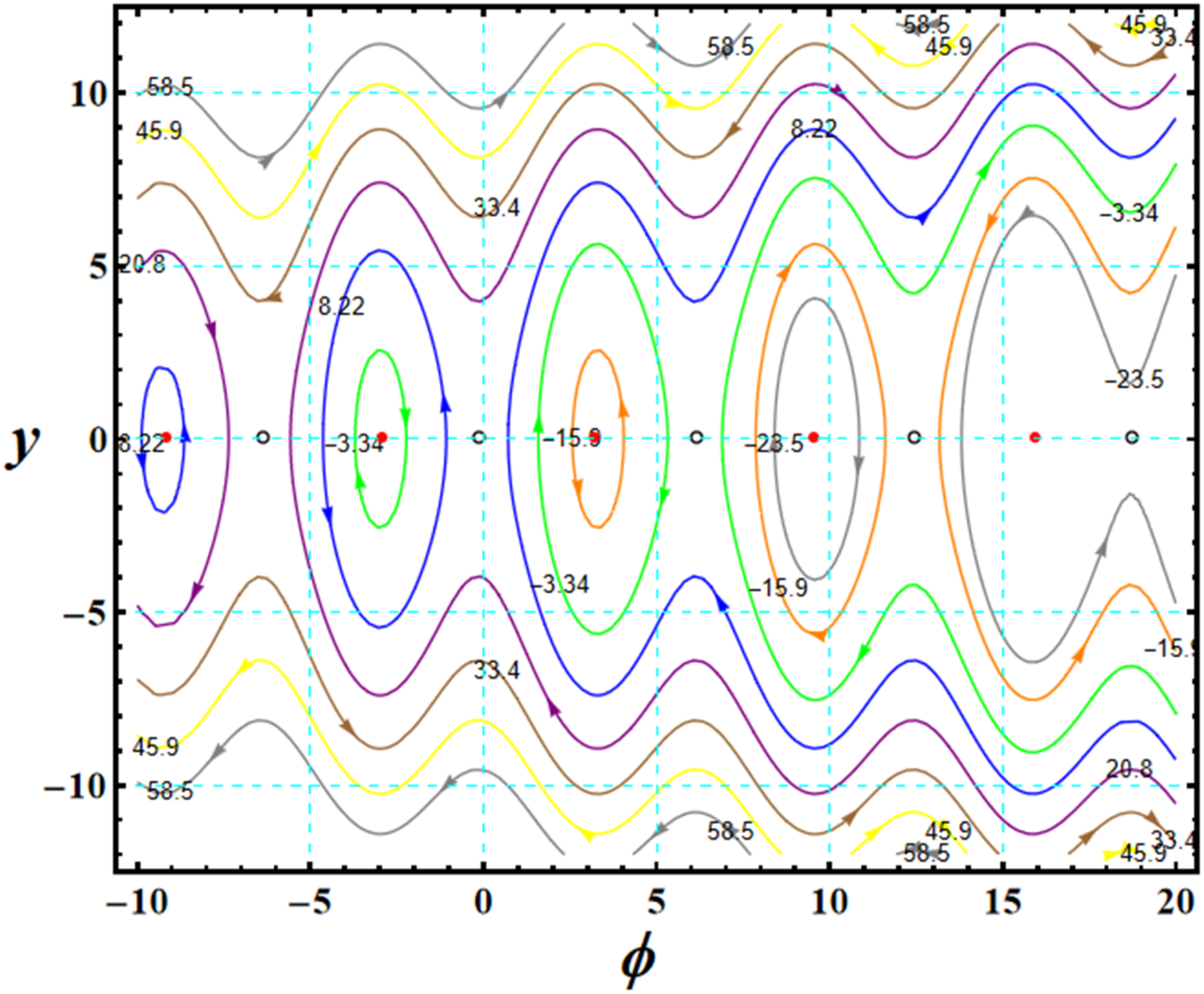
At an initial value $x\left(0\right)=\left(1.5,3,0.1\right)$ and at a principal inertia’s moment $D=\left(2000,1500,1000\right)\text{kg}.{\mathrm{m}}^2$ , Figure 12 presents a graph for the counterplots of some approached SS at ${\lambda }_2=100\text{kg}.{\mathrm{m}}^2.{\mathrm{s}}^{-1}.$ These SSs are $x_1\left(x_2-b\right)=-1,x_1+x_2+a=0,x_1^2-{\left(x_2+a\right)}^2+4\left(a+b\right)\left(x_2+a\right)-4\hspace{0.17em}{\tan }^{-1}\left[\left(x_2+a\right)/x_1\right]=0,$ and $\left[x_1^2+{\left(x_2+a\right)}^2\right]-4=0$ . The positions where the CP, SP, and VC points intersect with the RS and LS in Figure 11 correspond to the positions where a circle $B$ intersects with the CP, SP, and VC curves in Figure 12.

Figure 11.

A contour-mapping for stationary torque directed on the minor axis.

Figure 12.

Contour-maps of the LS and RS surfaces for a minor torque axis that remains constant.

To solve the transcendental equations given by (36), it is necessary to determine where the two SS intersect with the $\left(x_1,x_2\right)$ plane

$\cos \hspace{0.17em}{\varphi }_{\mathrm{s}}-\cos \hspace{0.17em}\varphi +4\left(a+b\right)\left\{\left[\cos \frac{{\varphi }_{\mathrm{s}}}{2}-\cos \frac{\varphi }{2}\right]/B\right\}+\left({\varphi }_{\mathrm{s}}-\varphi \right)\sin \hspace{0.17em}{\varphi }_{\mathrm{s}}=0\hspace{0.17em}.$

(40)

Assuming that $\varphi ={\varphi }_{\mathrm{s}}$ , is a solution of (38), which leads to

$\sin \hspace{0.17em}{\varphi }_s=\sin \hspace{0.17em}\varphi =\frac{2\hspace{0.17em}\tan \left(\varphi /2\right)}{1+{\tan }^2\left(\varphi /2\right)}=\frac{2x_1\left(x_2+a\right)}{x_1^2+{\left(x_2+a\right)}^2}.$

(41)

A detailed representation of the maximum and minimum values of the NAVCs is approached (see Appendix B).

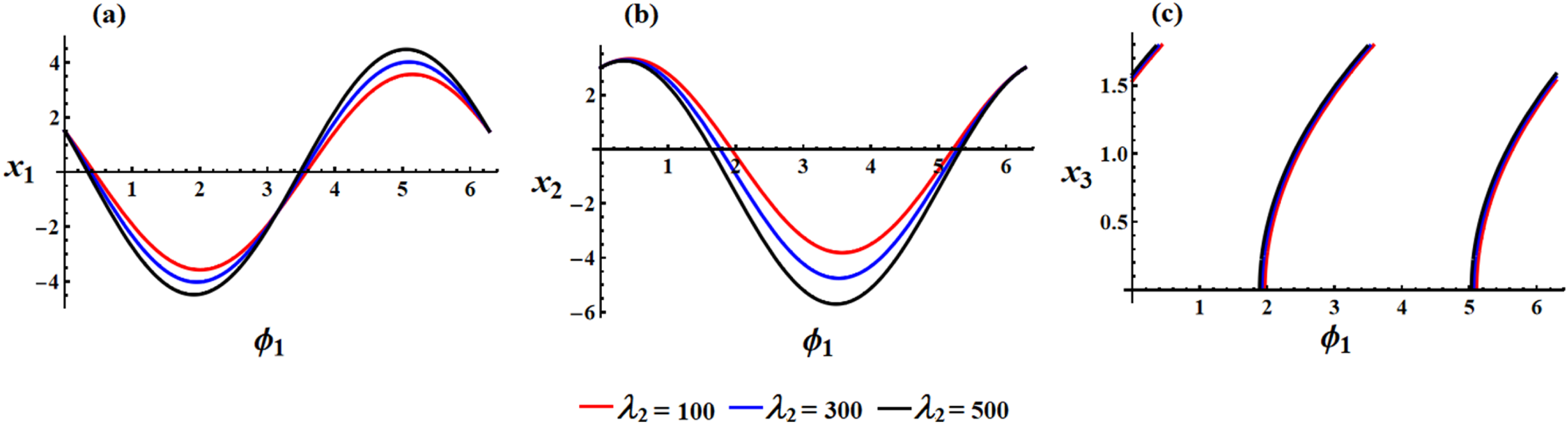
Figure 13 shows a simulation for the solutions in (31) and (39) for the NAVCs $x_1$ , $x_2$ , and $x_3$ in a period ${\theta }_1\in \left[0,2\pi \right]$ as ${\lambda }_2=\left(100,300,500\right)\text{kg}.{\mathrm{m}}^2.{\mathrm{s}}^{-1}$ . In Figure 13(a), the three graphs exhibit a periodic, oscillating pattern, indicating that when the angular displacement ${\varphi }_1$ grows, the angular velocity $x_1$ oscillates. The oscillations in $x_1$ exhibit a higher amplitude as the GT increases from 100 to 500. This suggests that when ${\varphi }_1$ rises, larger GT results in more pronounced changes in $x_1$ . While the intensity (amplitude) of the oscillations varies, the phase (the locations of the peaks and troughs) of the oscillations is almost the same for all three curves, indicating that the oscillatory behavior is constant across various GTs.

Figure 13.

The solution of the NAVCs at ${\lambda }_2=\left(100,300,500\right)\text{kg}.{\mathrm{m}}^2.{\mathrm{s}}^{-1}$ for a steady minor torque axis.

The graphed curves in Figure 13(b) show periodic, oscillatory behavior, implying that $x_2$ undergoes continuous oscillations as ${\varphi }_1$ increases. As the GT increases from 100 to 500, the amplitude of the oscillations in $x_2$ grows. This means that $x_2$ becomes more sensitive to changes in ${\varphi }_1$ as the GT increases. The phase (location of peaks and troughs) is consistent across all curves, meaning that the oscillation pattern remains unchanged regardless of the GT, but the magnitude of the oscillations differs.

Figure 13(c) shows that the GT has a direct effect on the system’s rotational dynamics, particularly in how fast $x_3$ increases as a function of ${\varphi }_1$ . As the GT increases, the system becomes more dynamic, exhibiting faster changes in angular velocity.

Based on the aforementioned analysis, it is important to understand how rotational motion can be stabilized or manipulated through the use of gyrostatic effects. Lower GT results in more controlled, gradual changes, which may be beneficial in systems requiring smooth and stable rotations. On the other hand, higher GT introduces a faster, more responsive dynamic, which may be needed in systems requiring agile and quick rotational responses.

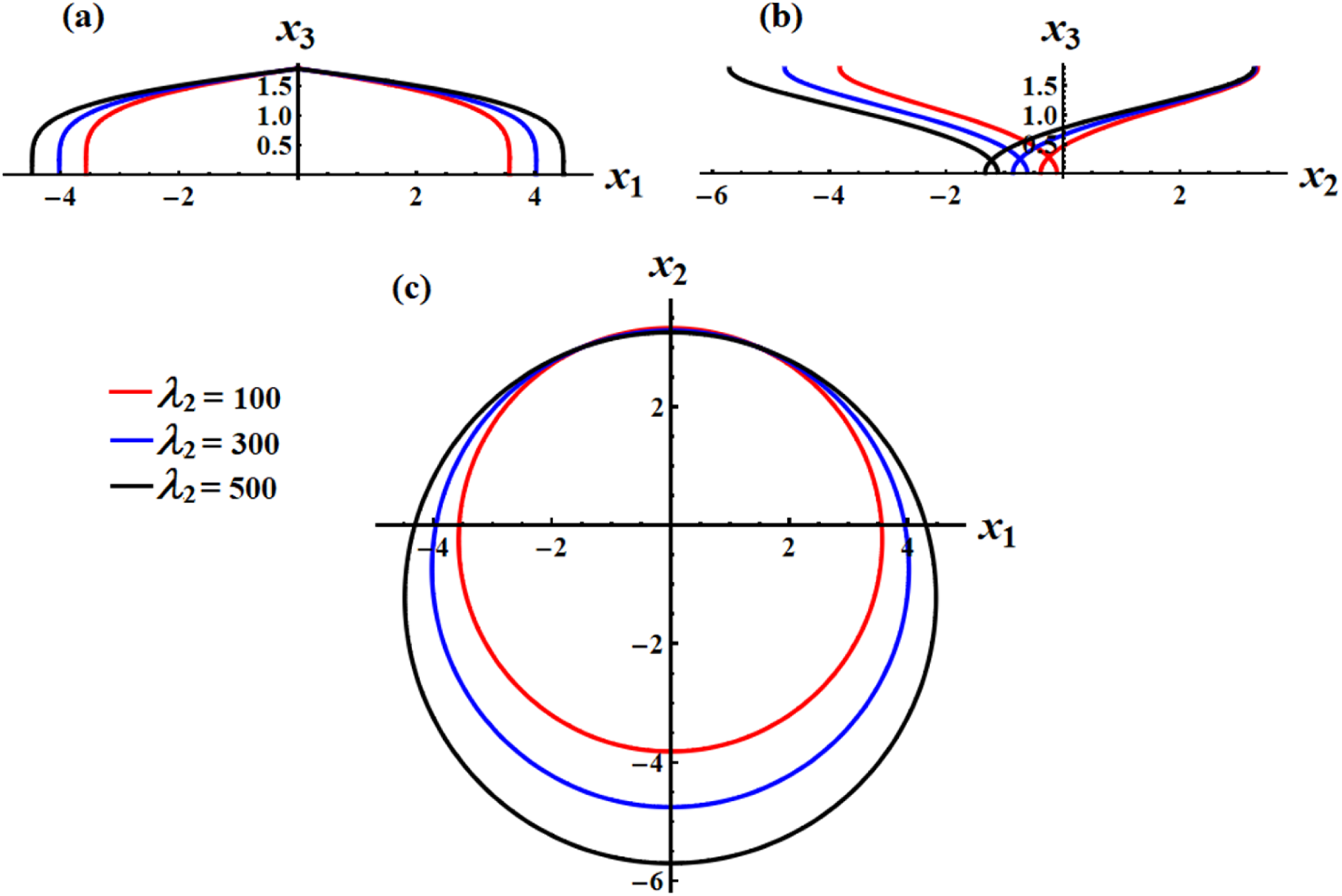
Figure 14(a) shows that as the GT increases; the corresponding curve moves outward. This means that for higher GT, the system exhibits a broader range of angular velocity components. All curves are symmetric about the vertical axis $\left(x_1=0\right)$ , indicating that the relationship between $x_1$ and $x_3$ is consistent in both positive and negative directions of $x_1$ .

Figure 14.

Parametric plots representing the relationship between $x_1$ , $x_2$ , and $x_3$ for a steady minor torque axis.

In Figure 14(b), as the GT increases, the curves spread out more, particularly in the $x_2$ direction. This suggests that the range of $x_2$ increases with higher GT. The curves display a distinct asymmetric shape about the vertical axis $\left(x_2=0\right)$ . Unlike the previous plot involving $x_1$ and $x_3$ , the relationship between $x_2$ and $x_3$ is not symmetric, indicating different dynamical behavior in the positive and negative $x_2$ directions.

In Figure 14(c), the curves form nearly circular shapes, with the size of the circle increasing as the GT increases. This suggests that the system allows for larger magnitudes of $x_1$ and $x_2$ as the GT becomes greater. The increase in the radius of the circles with increasing GT indicates that the system’s ability to achieve higher angular velocities in both $x_1$ and $x_2$ directions are enhanced by the larger GT.

Constant body torque in the middle axis case

At $\left({\mu }_1,{\mu }_2,{\mu }_3\right)=\left(0,1,0\right),$ system (8) becomes

$d{x}_1/d\tau =x_2{x}_3+a{x}_3, d{x}_2/d\tau =1-x_3{x}_1, d{x}_3/d\tau =x_1{x}_2-b{x}_1.$

(42)

To find the critical points of the system, Setting $d{x}_1/d\tau ,d{x}_2/d\tau ,$ and $d{x}_3/d\tau$ to zero, yields

$X_2{X}_3+a{X}_3=0, X_3{X}_1=1, X_1{X}_2-b{X}_1=0.$

From the first equation of the above system, we get $X_3=0$ and $X_2=-a$ . If $X_3=0$ , the second equation produces $X_3{X}_1-1=0$ , but −1 is not equal to zero. Consequently, $X_3\ne 0$ and $X_2=-a$ . Taking into account the third equation at $X_2=-a$ , one obtains $\left(a+b\right)X_1=0$ . Thus, $X_1=0$ if $a+b\ne 0$ . Finally, the second equation gives $-1=0$ , which is incorrect. Then there are no critical points if $a+b\ne 0$ . Therefore, we have two conclusions in this point:

(1) If $a+b=0$ , then $X_1$ is not restricted, and we would need to substitute $X_2=-a$ and check consistency with $X_1$ and $X_3$ in other equations to find any possible critical points.

(2) If $a+b\ne 0$ , there are no critical points.

A numerical approach (Runge–Kutta 4^th order Method) is employed to solve the system and observe how the GT effects on the rotational motion of the RB geometrically in some graph, which have been simulated according to the following data $D=\left(2000,1500,1000\right)\hspace{0.17em}\text{kg}.{\mathrm{m}}^2,$ and ${\lambda }_2=\left(100,300,500\right)\hspace{0.17em}\text{kg}.{\mathrm{m}}^2.{\mathrm{s}}^{-1},$ as in ⁵ .

For system (42) when $a+b\ne 0$ , the solution for the NAVCs $x_1$ , $x_2$ , and $x_3$ under the impact of a GT is presented in Figure 15. In addition to a phase-plane diagram that gives an induction about the stability of these solutions, as graphed in Figure 16. Inside the interval $\tau \in \left[0,15\right]\mathrm{s},$ the initial condition that is used to solve the system and represent these simulated diagrams is $x\left(0\right)=\left(1.5,3,0.1\right).$

Figure 15.

The time history of the NAVCs when ${\lambda }_2=\left(100,300,500\right)\hspace{0.17em}\text{kg}.{\mathrm{m}}^2.{\mathrm{s}}^{-1}$ at a constant middle axis.

Figure 16.

Phase-plane plots concerning the NAVCs $x_1$ , $x_2$ , and $x_3$ of Figure 15.

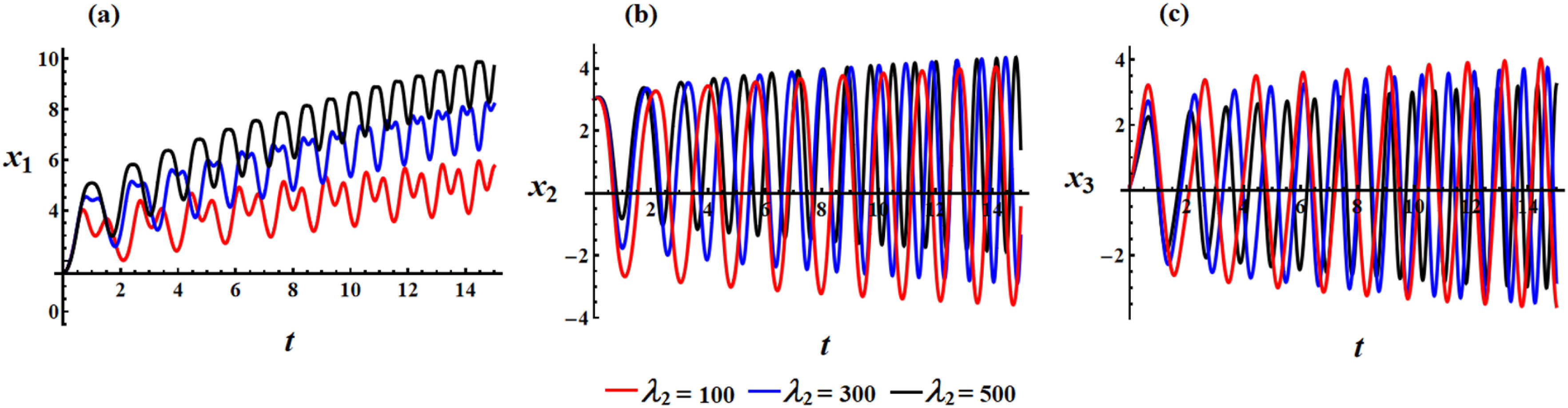
Figure 15(a) demonstrates how $x_1$ changes over time for different values of the GT. The largest values of the GT lead to larger and faster oscillations in $x_1$ , indicating that the system becomes more dynamic and responsive. For practical applications, adjusting the GT can control the system’s sensitivity to rotational changes, allowing for fine-tuned control over its behavior.

Figure 15(b) provides insight into the relationship between the solution of $x_2$ and ${\lambda }_2$ . As the GT increases, the oscillation frequency of $x_2$ increases, while the amplitude of oscillations decreases, which suggests that systems with larger GT become more stable, with less dramatic changes in $x_2$ - value over time.

Figure 15(c) explores that as the GT increases, the oscillations in $x_3$ become more frequent and less pronounced. Therefore, any system with larger GT experiences more stable rotational behavior, with smaller variations in $x_3$ over time.

Figure 16(a) represents the 3D simulation for the impact of the GT on the solutions of the NAVCs with respect to Figure 15. Figure 16(b) illustrates the phase plane of $x_1$ as the GT increases. The system’s response to torque increases involves larger oscillations in $x_1$ and $x_1^{\prime }$ . The curves remain elliptical, suggesting the system remains stable, though its behavior becomes more dynamic and less constrained, as the torque increases from 100 to 500. This could be indicative of a physical system such as a gyroscope or rotating RB, where increasing the external torque causes more pronounced oscillatory behavior.

The graphed phase plane in Figure 16(c) explores how $x_2$ respond to increasing GT. Higher torques (500, black curve) result in larger values of $x_2$ , while $x_2^{\prime }$ remains comparatively constrained. The elliptical trajectories indicate bounded oscillations, and the system remains stable and semi-periodic for all torque values analyzed. This behavior is typical of systems with rotational inertia, where increasing torque leads to greater rotational speeds while maintaining control over $x_2^{\prime }$ .

In Figure 16(d), the phase plane plots for $x_3$ shows how the system’s NAVC and its time derivative evolve as the GT increases from 100 to 500. The NAVC $x_3$ increases significantly with higher torque values, especially for the black curve (500 torque), where it reaches up to ±40. However, the $x_3^{\prime }$ remains relatively constant, showing a bounded oscillatory behavior. The distortion in the black curve suggests that at higher torques, nonlinear effects may become more significant, but the system remains stable and oscillatory for all torque levels analyzed.

This type of behavior could be characteristic of systems like gyroscopes or rotating RBs, where higher external torque leads to greater velocities, but the system remains controlled in its acceleration response.

For the system as $a+b=0$ , the solution for the NAVCs $x_1$ , $x_2$ , and $x_3$ under the impact of a GT is presented in Figure 17. In addition to a phase-plane diagram to show the stability of these solutions, graphed in Figure 18.

Figure 17.

The time history of the NAVCs when ${\lambda }_2=\left(100,300,500\right)\hspace{0.17em}\text{kg}.{\mathrm{m}}^2.{\mathrm{s}}^{-1}$ at a constant middle axis.

Figure 18.

Phase-plane plots concerning to the NAVCs $x_1$ , $x_2$ , and $x_3$ of Figure 17.

In Figure 17(a), as the GT increases (from 100 to 500), the amplitude of the angular velocity oscillations increases, while the frequency of oscillations decreases. The graph illustrates how $x_1$ becomes more pronounced and slower in oscillation, as the GT increases. This indicates that larger GT leads to larger and slower oscillations in $x_1$ , which can be a critical factor when studying gyroscopic systems, such as instability analysis or rotational dynamics.

A closer look at the plotted curves in Figure 17(b) indicates that as the GT increases (from 100 to 500), the amplitude of $x_2$ increases, while the frequency of the oscillations decreases. The black curve (highest GT) exhibits the widest oscillations, while the red curve (lowest GT) has the most frequent oscillations but with a smaller range. All three curves maintain relatively regular oscillatory behavior, but the amplitude and frequency differ depending on the value of the GT. This pattern indicates that the behavior of $x_2$ , like $x_1$ , is significantly influenced by the GT. Higher GTs result in slower, larger oscillations in $x_2$ , which could be relevant in understanding rotational stability or dynamic behavior in any system, where the GT varies.

In Figure 17(c), as the GT increases (from 100 to 500), the amplitude of the oscillations in $x_3$ increases, while the frequency of oscillations decreases. The red curve, representing the smallest GT, has the smallest amplitude and the highest frequency, with rapid oscillations over time. The black curve, representing the largest GT, has the largest amplitude and the slowest oscillations, with fewer cycles across the time range. The blue curve falls between the red and black in both amplitude and frequency, exhibiting moderate oscillations in both aspects. This behavior suggests that $x_3$ , like the other components ( $x_1$ and $x_2$ ), becomes slower and exhibits larger oscillations as the GT increases.

These changes in behavior could have significant implications in the analysis of gyroscopic systems, especially in contexts involving dynamic stability or rotational motion, where varying GTs influence angular velocities.

Figure 18(a) represents the 3D simulation of the GT impact on the solutions of the NAVCs with respect to Figure 17. Figure 18(b) plots phase trajectories for $x_1$ as it evolves under different GT values. As the GT increases, the system undergoes changes in its dynamic behavior. The elliptical shapes seen in the graph suggest that the system exhibits periodic motion, with $x_1$ oscillating stably around an EP. The size of the ellipses varies based on the applied GT. The trajectories demonstrate stable oscillatory behavior, as seen from the closed ellipses. This suggests the system is not chaotic for the given range of torques and remains within a bounded region of phase space. The graph shows how increasing GT leads to larger oscillations in $x_1$ , suggesting that higher gyrostatic effects increase the rotational response of the system, but without causing instability in the dynamics.

Figure 18(c) depicts closed curves (phase trajectories) for different GT values. These trajectories reflect the periodic nature of the rotational motion, where $x_2$ oscillates with varying amplitude and frequency, depending on the GT. The ovals become wider as torque increases, signifying greater angular velocities and accelerations in the system. This shows that as GT increases, the RB responds with more significant rotational dynamics, but it does not exhibit chaotic behavior.

In Figure 18(d), the shapes in this phase plane graph have a characteristic wavy appearance, unlike the more regular elliptical shapes seen in the previous two graphs. These wavy contours suggest that the dynamics of $x_3$ involve more complex oscillatory motion compared to $x_1$ and $x_2$ . The wavy nature of the phase trajectories suggests a more intricate relationship between $x_3$ and $x_3^{\prime }$ compared to the smoother ellipses seen in previous graphs. This may indicate the presence of nonlinear effects or higher-order terms influencing the system’s dynamics along the third axis.

Despite the increased complexity, the curves remain closed, signifying stable, periodic motion. As with the other graphs, the system does not display chaotic behavior for these GT values, although the dynamics become more pronounced with increasing GT.

In comparing the current study with those previously studied the problem referenced in [4] without the GT and [5] in the presence of the first component of the GT only, several key differences and similarities emerge. This comparison is presented in the following Table 2:

Table 2.

Comparison between this work and previous ones in Refs. 4 and 5.

Case	Comparison items	The present study	Ref. [4]	Ref. [5]
Problem formulation	Description	Study the rotational motion of the RB under external torques and the second component of the GT	Study the rotational motion of the RB under external torques	Study the rotational motion of the RB under external torques and the first component of the GT
Constant body torque in the major axis case	Analytical solution for the angular velocities	Approached	Approached	A numerical solution is derived
	Stability analysis	Approached	Not approached	Not approached
	Equilibrium and critical points	Calculated	Not calculated	Not calculated
	External forces acted on the body	CBFTs and the second component of the GT	CBFTs	CBFTs and the first component of the GT
	Maximum and minimum values	Estimated	Estimated	Not estimated
Constant body torque in the minor axis case	Analytical solution for the angular velocities	Approached	Not approached	Approached
	Stability analysis	Approached	Not approached	Estimated
	Equilibrium and critical points	Calculated	Not calculated	Calculated
	External forces acted on the body	CBFTs and the second component of the GT	CBFTs	CBFTs and the first component of the GT
	Maximum and minimum values	Estimated	Estimated	Estimated
Constant body torque in the middle axis case	Analytical solution for the angular velocities	A numerical solution is derived	Approached	Approached
	Stability analysis	Approached	Not approached	Approached
	Equilibrium and critical points	Calculated	Not calculated	Calculated
	External forces acted on the body	CBFTs and the second component of the GT	CBFTs	CBFTs and the first component of the GT
	Maximum and minimum values	Not estimated	Estimated	Estimated

Despite these differences, all three studies contribute to advancing the understanding of the problem of the RB’s rotational motion, making the comparison particularly valuable for readers interested in the nuances of the RB’s rotary motion. The future work of this study will be very complicated as we intend to study the problem with a time-varying GT or supplying the system with three external rotors with different torques affecting the motion of the RB to see various aspects of its dynamical behavior under these conditions.

Conclusion

In this paper, analytical and asymptotic solutions for the RB motion influenced by GT and BCFTs, are presented. The scaled form of Euler’s EOM is used as the governing EOM for the RB. In the case of BCFTs, the EOMs are nondimensionalized to reduce their dependence on the torque magnitude and the inertia qualities. EPs of the non-dimensional system are identified, along with the linearized EOMs, characteristic equation, and stability characteristics. In both cases of BCFT along the major and minor axes, the analytical solution for the case was addressed through a comprehensive simulation that included diagrams for the steady state, paths, stability regions, and extreme values. In the case of BCFT along the central axis, a numerical solution is examined, along with two and three-dimensional graphs depicting the NAVCs, which result in a typical spin-up maneuver observed in some of the initially investigated regions. In contrast, in the second set of regions, the motion’s stability shifts as the GT increases, transitioning to either a stable or unstable state depending upon the GT value. The extreme value of the case is also examined, with stabilization addressed in two sections. Each section offers a solution and includes a table of extreme values within the stable separatrix region. Additionally, the influence of distinct GT values on motion paths and stabilization is analyzed, yielding valuable insights for this scenario. For each case, a comprehensive estimation of the maximum and minimum values at distinct NAVCs along a periodic solution is approached. This study has the potential to significantly influence the industries of spaceships and satellites by deepening our understanding of rotary motion and contributing to a thorough comprehension of the behavior of celestial bodies. The research will conclude with an extensive report that clarifies the complexities of rotary and orbital motion.