Dynamical motion of a spacecraft containing a slug and influenced by a gyrostatic moment and constant torques

Abstract

This study examines how a spacecraft reacts to constant body-fixed torques and a gyrostatic moment (GM), as well as the impact of energy dissipation. The spacecraft model being studied includes a spherical slug near the center of mass covered by a viscid layer. The problem’s difficulty lies in solving its governing equations of motion (EOMs), which are derived through Euler nonlinear equations. Understanding the behavior of this model can offer insights into how spacecraft respond to external torques, aiding in the development of more efficient and stable systems for aerospace and robotics applications. The research delves into the relationship between energy dissipation and GM on the spacecraft motion in three different scenarios involving constant torques around three various axes. Detailed analysis, as well as novel solution and simulation results, are presented for different energy dissipation possibilities. The influence of manipulating the value of the GM and the viscosity of the layer has been approached. These findings are crucial for comprehending, maintaining, and controlling the motion of spacecraft influenced by external forces in space. The study promises to have a significant impact on the aerospace industry, particularly in the design and operation of spaceships and satellites, by enhancing our knowledge of rotational motion and celestial bodies’ behavior. A comprehensive report will be produced to elucidate the complexities of rotational and orbital motion discovered during this research.

Introduction

Studying the dynamics of rigid bodies (RGBs) like spacecraft subject to external torques, energy dissipation, and GM plays a significant role in calculating the angular velocity trajectories of its rotary motion. In disciplines where stable and effective system designs are crucial, including robotics and aircraft, the behavior of these systems is crucial. As a result, in order to understand how these bodies rotate, one must look into how GM and energy dissipation affect their dynamics. This is especially true for semi-RGBs that undergo internal energy dissipation, where it’s critical to realize that kinetic energy gradually decreases. Consequently, the energy ellipsoid will gradually shrink, forming an open polychromatic spiral pathway that deviates from the minor axis of the RGB. As this pathway crosses the separatrix and approaches the major axis, the RGB will inevitably reposition and rotate about its major axis with an upward or downward spin rate. Owing to their intrinsic instability, RGBs that rotate about their minor axis when energy dissipation occurs require close observation and adjusting to maintain stability and prevent any possible catastrophes or breakdowns. For practical purposes, the RGB must consequently often be designed within this manner.

The dynamics of the motion of these bodies under the influence of external forces and torques with lots of different models have taken a lot of researchers’ interest in the past few years.^1–32 The influence of energy dissipation on this problem has been presented in Ref. 1–3. In Ref. 1, directional instability occurs when a spacecraft is rotating about its minor axis and energy dissipation is present. The author shows that the maneuver gives the appropriate final orientation when it is combined with two thruster firings that are based on gyro readings. In Ref. 2,3, three different scenarios for major, minor, and middle axes corresponding to the influence of constant body-fixed torques, ² and the GM. ³ The authors have approached the analytical and numerical solutions for the RGB angular velocity component in each scenario. In 4, the authors examine the rotary motion of a spaceship spinning up and thrusting during a maneuver where it is subjected to persistent body-fixed moments about all three axes. In order to produce simplified, useful formulas that shed light on the motion, the authors construct asymptotic and limiting-case expressions from the analytic solutions and study the evolution of the motion firstly as the time grows infinitely, and secondly for geometric examples of the thin plate, the thin rod, and the sphere. In Ref. 5, the process of launching the rotation of an axial symmetrical spacecraft while it is subjected to an exterior torque that is parallel to the symmetrical axis is examined. This problem is first solved using the exact analytic solution for an axially symmetric RGB which holds for any initial angular velocity and attitude, as well as any duration and rotation amplitude. A new approximation solution that was derived from the exact one is introduced. In Ref. 6, the stable orbit of a constantly rotating asteroid is considered a generalization of a fundamental issue of orientation stabilization in a central gravitational field. The differential geometrical approach is used to obtain the Poisson tensor, Casimir functions, and EOMs that control the system’s phase flow and phase space structures. Based on a global perspective, the equilibrium of EOMs, or the equilibrium attitude of the spacecraft, is found. This correlates to a stable point of the Hamiltonian that is limited by Casimir functions. In Ref. 7, the authors provide a basic framework for simulating RGB potentials that may be used, independent of gravity estimate techniques, to analyze the orbit–attitude coupling movement of a spacecraft near minor celestial objects. In Ref. 8, semi passive attitude stabilizing technique for a spacecraft in an orbital Keplerian trajectory within the electromagnetic field is described. The electrodynamic impact caused by Lorentz forces operating on the outermost layer of the charged spacecraft serves as the basis for the technique’s evolution. In Ref. 9, an asymptotic study presents an innovative technique for estimating the EOMs of a limited-sized satellite that is expected to be orbiting around the earth and in close range to it: the elliptical constrained 3-body problem, or ER3BP. In contrast, the approach used for resolving the EOMs at collinear sites {L₁, L₂} is described in Ref. 10. In Ref. 11, the authors investigate the rapid rotary movement near the mass center of an antisymmetric spacecraft subject to drag and gravitational torques. The EOMs which are generated after applying averages over Euler-Poinsot equations ¹² are explored. They find that there are semi-stationary phases for movement and that the modulus of angular momentum and kinetic energy fall.

In Ref. 13, another model considering Euler-Poinsot equations is presented for a fast rotation of unsymmetric satellites. Both analytic investigation and numerical evaluation in the general scenario are completed in the region of the axial rotation. In Ref. 14, the authors take into account the torque of a resisting force, constant torques, and the impact of GM on the RGB movement. The controlling EOMs are generated in an acceptable form by Euler’s equations. To get close to an appropriate form of motion controlling construction, the averaging technique is employed. To get to the necessary findings, several initial circumstances are taken into consideration besides applying Taylor’s method to find a solution for the obtained EOMs. In addition to the numerical evaluation, the asymptotic techniques used for solving EOMs allow us to get the ideal solutions for the problem. In Ref. 15, the authors expand on their earlier findings for the problem ¹⁴ when subjected to low interior or exterior torques. One could argue that this investigation mainstreams. ¹⁴ This study has the advantage of providing both the original asymptotic and numerical solutions that, with a simultaneously tiny error, describe the progress of motion of RGB with a moving mass. In Ref. 16, the free angular movement of coaxial RGBs and the orientation of spacecraft duple-spinning are studied. A few heteroclinic chaotic scenarios are explained. Based on the Melnikov approach and Poincare maps, the regional chaotization of the spacecraft is estimated in the presence of polyharmony perturbations and modest nutation restoring/overturning torques. In Ref. 17, the most effective approach to managing a spacecraft’s kinetic torque during an orientation movement from an unspecified initial to a specified ending angular position while accounting for rotational energy requirements is examined. The optimum regulation of spacecraft reorientation is solved analytically. For the purpose of creating an ideal control program, structured EOMs are provided. The turning control problem has been resolved considering the constraints on the control torques. The maximal rotational energy and the turning time were discovered to be analytically related.

In Ref. 18, the authors take into consideration the orientation kinematics of a shifting mass spacecraft. The performance of an aircraft engine, which creates an interorbital impulse, is linked to the variation of mass-inertia characteristics across time. In order to complete the nutational precessional movement in relation to a predetermined direction in the inertial space, the aircraft engine’s thrust travels along its longitudinal axis. Therefore, it is necessary to generate a movement zone with a monotonically lowering nutation angle in order to maximize the precision of the thrust impulse production during the engine performance and to reduce the thrust dispersion caused by the precessional spin. In Ref. 19, an analysis was conducted on the feasibility of employing the electrodynamic control system to achieve monoaxial stability for a satellite in an indirectly orbiting coordinate frame. It was proposed to expand the idea of electrodynamic control and provide a solution for the electrodynamic correction of the perturbing torque. In Ref. 20, an analysis is done on the viability of employing an electrodynamic orientation control system for the orbiting coordinate system’s monoaxial orientation stability of artificial Earth satellites. It is suggested that the idea of electrodynamic control of orientation be developed, using a restorative torque with a dispersed delay. In Ref. 21, the study looks at the kinematics of free motion in duple-spinning spacecraft and gyrostatic satellites. In regard to Jacobi elliptic functions, unique analytical solutions for the components of the angular velocity and Euler angles are derived.

In Ref. 22, the solutions for the governing EOMs for the kinematics of 3D rotary motion of the RGB under the impact of the third component of the GM, electromagnetic field, time-varying, and constant components of a stationary torque are estimated. As well Euler angles have been calculated through the obtained solutions and the assumption of the small angle approximation. In Ref. 23, in addition to the GM influence, the author presents the periodic analytical solution for the problem with the impact of a Newtonian field using the small parameter technique of Poincare. In Ref. 24, for the kinematics of a charged unsymmetric model of the RGB, the exact solutions for the RGB’s angular velocity, Euler angles, both transverse and axial velocity, and displacement are approached with graphical simulations for these outcomes. In Ref. 25, inside Newtonian and electromagnetic fields, a small parameter technique is used to approach the asymptotic solution for the RGB motion under perturbating, restoring, and gyroscopic torques. In Ref. 26, the Krylov-Bogoliubov-Mitropolski technique is used to approach the solution for a charged model of the RGB influenced by GM. In Ref. 27, the solution is approached for a nearly symmetric model for the RGB with constant torques and the GM. In Ref. 28–30, the authors in these studies approach the solution for the problem by using the Homotopy perturbation method. In Ref. 28, an estimated frequency solution for the fractal rotational pendulum oscillator has been obtained using He’s frequency formula. In Ref. 29, a general method for building the homotopy equation and the initial guess. The Duffing oscillator is used as an example to demonstrate the method’s efficacy. In Ref. 30, a method that employs a novel canonical form for the SIR-epidemic system is introduced. In Ref. 31, the novel analytical solutions for the angular velocities for the RGB have been approached and visualized. Also, the effect of GM and the constant body-fixed torques on these obtained solutions has been presented. The stability and periodicity of the system’s angular velocities can be seen using phase portraits, which have also been investigated. In Ref. 32, the governing equations of how the RGB spins about a stationary point under the effect of the GM are described by Euler-Poisson’s dynamical equations, which can be solved in a different way. Using computer codes, the analytical solution to the problem is given and graphically represented, enabling us to examine the motion at any point in time. Additionally, the impact of GM’s unique values on these solutions is discussed.

This paper explores the motion behavior of a spacecraft during three distinct rotational maneuvers. Its rotary motion is investigated when the spacecraft is subjected to several forces, such as energy dissipation, constant torques, and GM, which serve as a crucial factor that influences the behavior of the spacecraft. Analyzing these forces and factors, we aim to gain a better understanding of the dynamics involved in these maneuvers and how they can be optimized for practical applications. The controlling EOMs are derived which allows us to analyze the difficulty of solving the problem. An approximate solution to the problem is derived with a full plot simulation for every possible situation the spacecraft could experience during the motion along the three axes. These results have an outstanding influence on designing and analyzing systems for satellites, spacecraft, and asteroids. Applications in fields like engineering and astrophysics would also be impacted by the findings. This research could serve as a model for future scholars to investigate other viewpoints for the GM in this specific scenario.

Problem’s formulation

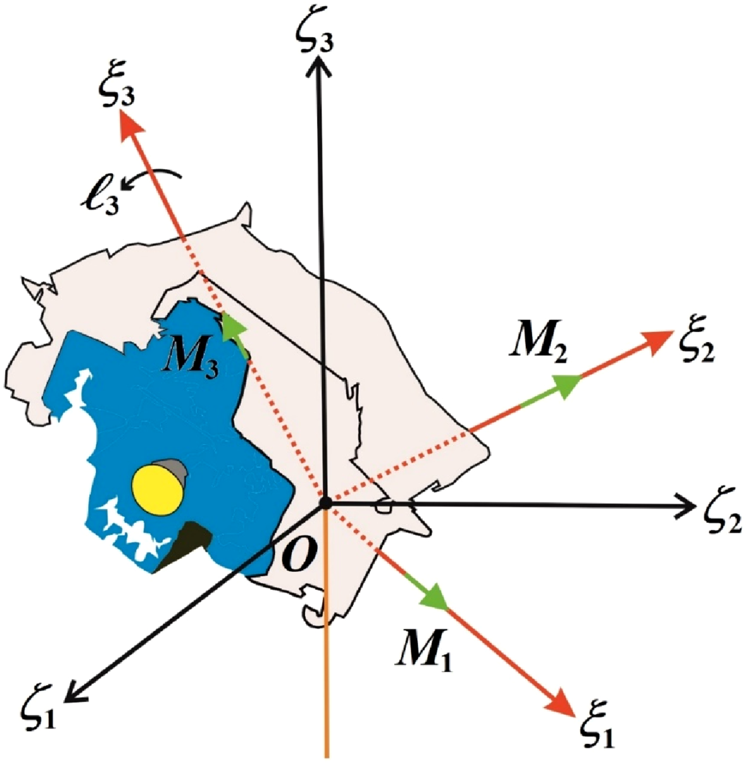
This section will provide an overview of the research problem which is the rotational motion of a spacecraft subject to constant fixed torques $\overline{\Omega }$ and the GM $\overline{\mathcal{l}}=\left(0,0,{\mathcal{l}}_3\right)$ . Two coordinate systems are taken into consideration; the fixed $O{\zeta }_1{\zeta }_2{\zeta }_3$ is the first and the rotating $O{\xi }_1{\xi }_2{\xi }_3$ is the second. To study the way energy dissipation affects the motion of this spacecraft, it has been taken into account that the spacecraft model has a slug of inertia $Q$ with a spherical shape near the spacecraft mass center. This slug is also encircled by a viscid layer which has a viscosity parameter $\lambda$ . A fully simulated model of the spacecraft is presented in Figure (1).

Figure 1.

The spacecraft’s model.

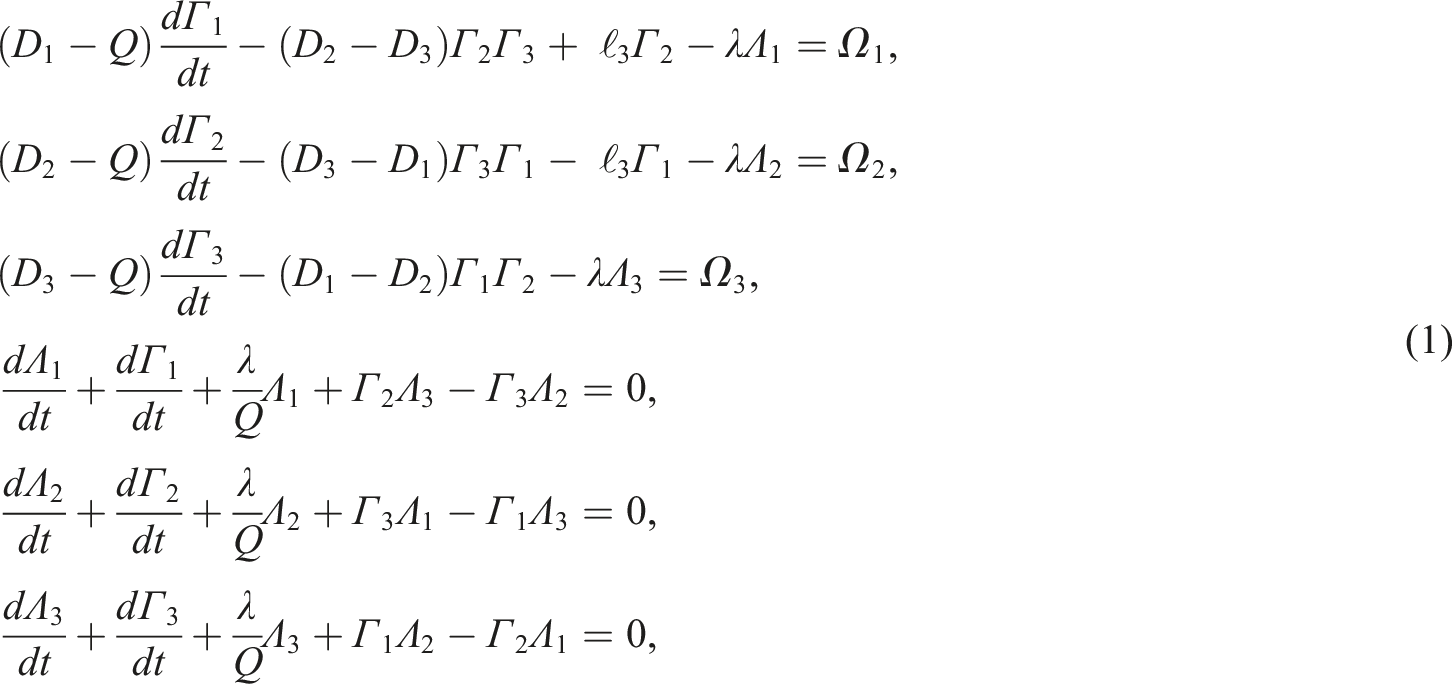
The controlling EOMs for the spacecraft rotary motion are given by^3,12:

$\begin{array}{l}\left(D_1-Q\right)\frac{d{\Gamma }_1}{dt}-\left(D_2-D_3\right){\Gamma }_2{\Gamma }_3+{\mathcal{l}}_3{\Gamma }_2-\lambda {\Lambda }_1={\Omega }_1,\\ \left(D_2-Q\right)\frac{d{\Gamma }_2}{dt}-\left(D_3-D_1\right){\Gamma }_3{\Gamma }_1-{\mathcal{l}}_3{\Gamma }_1-\lambda {\Lambda }_2={\Omega }_2,\\ \left(D_3-Q\right)\frac{d{\Gamma }_3}{dt}-\left(D_1-D_2\right){\Gamma }_1{\Gamma }_2-\lambda {\Lambda }_3={\Omega }_3,\\ \begin{array}{l}\frac{d{\Lambda }_1}{dt}+\frac{d{\Gamma }_1}{dt}+\frac{\lambda }{Q}{\Lambda }_1+{\Gamma }_2{\Lambda }_3-{\Gamma }_3{\Lambda }_2=0,\end{array}\\ \begin{array}{l}\frac{d{\Lambda }_2}{dt}+\frac{d{\Gamma }_2}{dt}+\frac{\lambda }{Q}{\Lambda }_2+{\Gamma }_3{\Lambda }_1-{\Gamma }_1{\Lambda }_3=0,\\ \frac{d{\Lambda }_3}{dt}+\frac{d{\Gamma }_3}{dt}+\frac{\lambda }{Q}{\Lambda }_3+{\Gamma }_1{\Lambda }_2-{\Gamma }_2{\Lambda }_1=0,\end{array}\end{array}$

(1)

where the spacecraft’s main inertia tensor is $D=\left(D_1,D_2,D_3\right)$ , and $D_1>D_2>D_3$ , the angular velocity vector corresponding to the spacecraft is represented by $\overline{\Gamma }=\left({\Gamma }_1,{\Gamma }_2,{\Gamma }_3\right)$ . The slug angular velocity vector is denoted by $\overline{\Lambda }=\left({\Lambda }_1,{\Lambda }_2,{\Lambda }_3\right)$ , and $Q$ symbols the inertia moment of the spherical slug where $D_j>Q,\left(j=1,2,3\right)$ , and ${\Omega }_j$ are the components of the constant torque $\overline{\Omega }$ , while ${\mathcal{l}}_3$ is the third component of the GM $\overline{\mathcal{l}}$ acting on the minor axis, and $t$ denotes the time.

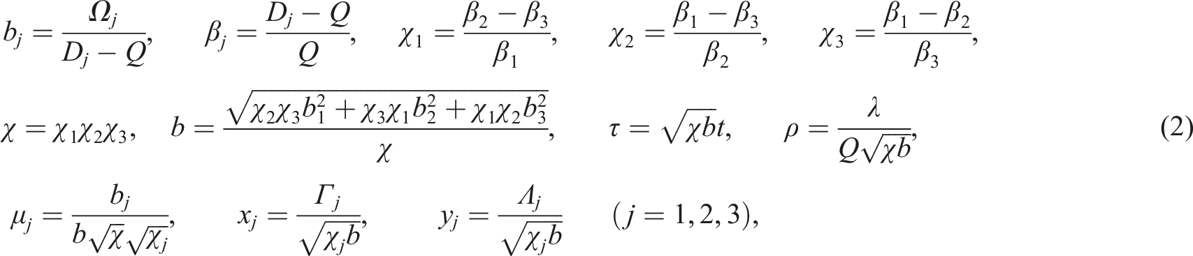
Introducing the following parameters

$\begin{array}{l}{b}_j=\frac{{\Omega }_j}{D_j-Q}, {\beta }_j=\frac{D_j-Q}{Q}, {\chi }_1=\frac{{\beta }_2-{\beta }_3}{{\beta }_1}, {\chi }_2=\frac{{\beta }_1-{\beta }_3}{{\beta }_2}, {\chi }_3=\frac{{\beta }_1-{\beta }_2}{{\beta }_3},\\ \chi ={\chi }_1{\chi }_2{\chi }_3, b=\frac{\sqrt{{\chi }_2{\chi }_3{b}_1^2+{\chi }_3{\chi }_1{b}_2^2+{\chi }_1{\chi }_2{b}_3^2}}{\chi }, \tau =\sqrt{\chi b}t, \rho =\frac{\lambda }{Q\sqrt{\chi b}},\\ {\mu }_j=\frac{b_j}{b\sqrt{\chi }\sqrt{{\chi }_j}}, x_j=\frac{{\Gamma }_j}{\sqrt{{\chi }_{j}b}}, y_j=\frac{{\Lambda }_j}{\sqrt{{\chi }_{j}b}} \left(j=1,2,3\right),\end{array}$

(2)

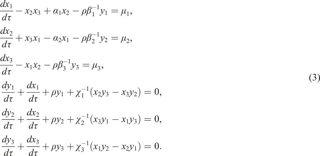
to simplify system (1) into

$\begin{array}{l}\frac{d{x}_1}{d\tau }-x_2{x}_3+{\alpha }_1{x}_2-\rho {\beta }_1^{-1}{y}_1={\mu }_1,\\ \frac{d{x}_2}{d\tau }+x_3{x}_1-{\alpha }_2{x}_1-\rho {\beta }_2^{-1}{y}_2={\mu }_2,\\ \frac{d{x}_3}{d\tau }-x_1{x}_2-\rho {\beta }_3^{-1}{y}_3={\mu }_3,\\ \begin{array}{l}\frac{d{y}_1}{d\tau }+\frac{d{x}_1}{d\tau }+\rho y_1+{\chi }_1^{-1}\left(x_2{y}_3-x_3{y}_2\right)=0,\\ \frac{d{y}_2}{d\tau }+\frac{d{x}_2}{d\tau }+\rho y_2+{\chi }_2^{-1}\left(x_3{y}_1-x_1{y}_3\right)=0,\\ \frac{d{y}_3}{d\tau }+\frac{d{x}_3}{d\tau }+\rho y_3+{\chi }_3^{-1}\left(x_1{y}_2-x_2{y}_1\right)=0.\end{array}\end{array}$

(3)

where ${\alpha }_1=\frac{{\mathcal{l}}_3}{Q{\chi }_1{\beta }_1\sqrt{{\chi }_{3}b}}$ , ${\alpha }_2=\frac{{\mathcal{l}}_3}{Q{\chi }_2{\beta }_2\sqrt{{\chi }_{3}b}}$ . It is noted that ${\beta }_j$ , $x_j$ , $y_j$ , ${\mu }_j$ , ${\mathcal{l}}_3$ , and $\tau$ are dimensionless quantities. ³ The dimensionless formula for the rotatory movement of the damped spacecraft is determined by the independent factors concerning the system (3), which are ${\beta }_j$ , ${\mathcal{l}}_3$ , $Q$ , and $\rho$ , lesser than the dimensional compared factors in the system (1), which are $D_j$ , $Q$ , ${\mathcal{l}}_3$ , and $\lambda$ . Recalling the formulae $b_j$ and $b$ in (2), the following formula is deduced as

${{\mu }_1}^2+{{\mu }_2}^2+{{\mu }_3}^2=1.$

(4)

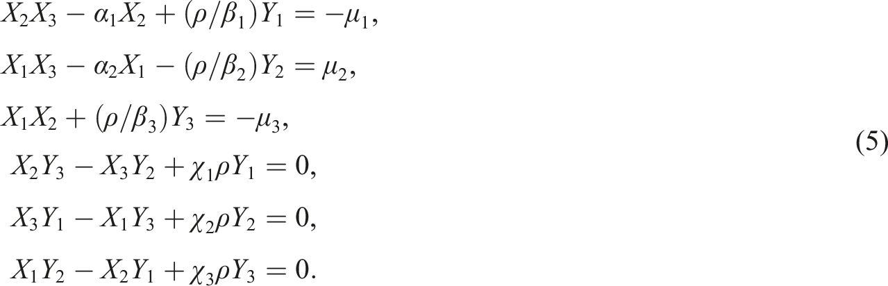
To approach the equilibrium state for the motion, the following derivatives $\frac{d{x}_j}{d\tau }$ , $\frac{d{y}_j}{d\tau }$ must put to equal zero, where $x_j=X_j$ , and $y_j=Y_j$ are the components of the equilibrium point (EP). Hence, system (3) gives

$\begin{array}{l}{X}_2{X}_3-{\alpha }_1{X}_2+\left(\rho /{\beta }_1\right)Y_1=-{\mu }_1,\\ X_1{X}_3-{\alpha }_2{X}_1-\left(\rho /{\beta }_2\right)Y_2={\mu }_2,\\ X_1{X}_2+\left(\rho /{\beta }_3\right)Y_3=-{\mu }_3,\\ \begin{array}{l}\begin{array}{l}{X}_2{Y}_3-X_3{Y}_2+{\chi }_1\rho Y_1=0,\\ X_3{Y}_1-X_1{Y}_3+{\chi }_2\rho Y_2=0,\\ X_1{Y}_2-X_2{Y}_1+{\chi }_3\rho Y_3=0.\end{array}\end{array}\end{array}$

(5)

Solving the 4^th, 5^th, and 6^th equations of (5) together, after some mathematical manipulation to obtain

${\beta }_1{Y}_1^2+{\beta }_2{Y}_2^2+{\beta }_3{Y}_3^2=0.$

(6)

With reference to equation (2), respecting both conditions $D_1>D_2>D_3$ and $D_j>Q$ implies that ${\beta }_j>0$ , as a result ${\chi }_j$ - values are positive. Consequently, it is only possible to satisfy equation (6) ² if and only if

$Y_1=Y_2=Y_3=0.$

(7)

Equations (6) and (7) can be substituted into (5) to produce

$\left(X_3-{\alpha }_1\right)X_2=-{\mu }_1, \left(X_3-{\alpha }_2\right)X_1={\mu }_2, X_1{X}_2=-{\mu }_3.$

(8)

With the further requirement of the EPs at the value of zero for $\left({\Lambda }_1,{\Lambda }_2,{\Lambda }_3\right)$ in the damped situation, we can observe that the EPs for the angular velocities are the same in both the damped and undamped situations.

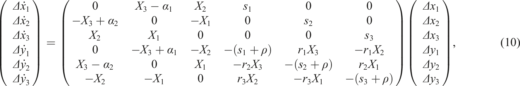
The perturbation state principle^13,14 can be defined as

$\Delta x_j=x_j-X_j, \Delta y_j=y_j-Y_j, \left(j=1,2,3\right).$

(9)

and taking into account ${\mu }_j$ ’s constancy, producing the linearized EOMs in the following way

$\left(\begin{array}{c} \Delta {\dot{x}}_1\\ \Delta {\dot{x}}_2\\ \Delta {\dot{x}}_3\\ \Delta {\dot{y}}_1\\ \Delta {\dot{y}}_2\\ \Delta {\dot{y}}_3\end{array}\right)=\left(\begin{array}{cccccc}0& X_3-{\alpha }_1& X_2& s_1& 0& 0\\ -X_3+{\alpha }_2& 0& -X_1& 0& s_2& 0\\ X_2& X_1& 0& 0& 0& s_3\\ 0& -X_3+{\alpha }_1& -X_2& -\left(s_1+\rho \right)& r_1{X}_3& -r_1{X}_2\\ X_3-{\alpha }_2& 0& X_1& -r_2{X}_3& -\left(s_2+\rho \right)& r_2{X}_1\\ -X_2& -X_1& 0& r_3{X}_2& -r_3{X}_1& -\left(s_3+\rho \right)\end{array}\right)\left(\begin{array}{l} \Delta x_1\\ \Delta x_2\\ \Delta x_3\\ \Delta y_1\\ \Delta y_2\\ \Delta y_3\end{array}\right),$

(10)

where $r_j={\chi }_j^{-1}$ , $s_j=\rho {\beta }_j^{-1}$ .

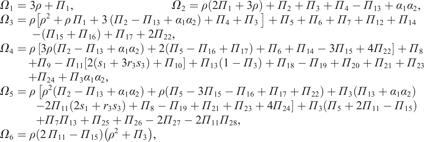
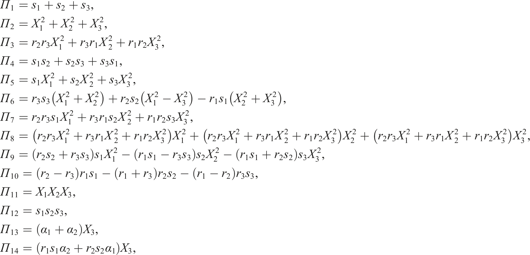
Therefore, the following formula can be used to write the characteristic equation of (10)

${\sigma }^6+{\Omega }_1{\sigma }^5+{\Omega }_2{\sigma }^4+{\Omega }_3{\sigma }^3+{\Omega }_4{\sigma }^2+{\Omega }_5\sigma +{\Omega }_6=0,$

(11)

$\begin{array}{l}{\Omega }_1=3\rho +{\Pi }_1, {\Omega }_2=\rho \left(2{\Pi }_1+3\rho \right)+{\Pi }_2+{\Pi }_3+{\Pi }_4-{\Pi }_{13}+{\alpha }_1{\alpha }_2,\\ {\Omega }_3=\rho \left[{\rho }^2+\rho \hspace{0.17em}{\Pi }_1+3\hspace{0.17em}\left({\Pi }_2-{\Pi }_{13}+{\alpha }_1{\alpha }_2\right)+{\Pi }_4+{\Pi }_3\hspace{0.17em}\right]+{\Pi }_5+{\Pi }_6+{\Pi }_7+{\Pi }_{12}+{\Pi }_{14}\\ -\left({\Pi }_{15}+{\Pi }_{16}\right)+{\Pi }_{17}+2{\Pi }_{22},\\ {\Omega }_4=\rho \hspace{0.17em}\left[3\rho \left({\Pi }_2-{\Pi }_{13}+{\alpha }_1{\alpha }_2\right)+2\left({\Pi }_5-{\Pi }_{16}+{\Pi }_{17}\right)+{\Pi }_6+{\Pi }_{14}-3{\Pi }_{15}+4{\Pi }_{22}\right]+{\Pi }_8\\ +{\Pi }_9-{\Pi }_{11}\left[2\left(s_1+3r_3{s}_3\right)+{\Pi }_{10}\right]+{\Pi }_{13}\left(1-{\Pi }_3\right)+{\Pi }_{18}-{\Pi }_{19}+{\Pi }_{20}+{\Pi }_{21}+{\Pi }_{23}\\ +{\Pi }_{24}+{\Pi }_3{\alpha }_1{\alpha }_2,\\ {\Omega }_5=\rho \hspace{0.17em}[{\rho }^2\left({\Pi }_2-{\Pi }_{13}+{\alpha }_1{\alpha }_2\right)+\rho \left({\Pi }_5-3{\Pi }_{15}-{\Pi }_{16}+{\Pi }_{17}+{\Pi }_{22}\right)+{\Pi }_3\left({\Pi }_{13}+{\alpha }_1{\alpha }_2\right)\\ -2{\Pi }_{11}\left(2s_1+r_3{s}_3\right)+{\Pi }_8-{\Pi }_{19}+{\Pi }_{21}+{\Pi }_{23}+4{\Pi }_{24}]+{\Pi }_3\left({\Pi }_5+2{\Pi }_{11}-{\Pi }_{15}\right)\\ +{\Pi }_7{\Pi }_{13}+{\Pi }_{25}+{\Pi }_{26}-2{\Pi }_{27}-2{\Pi }_{11}{\Pi }_{28},\\ {\Omega }_6=\rho \left(2\hspace{0.17em}{\Pi }_{11}-{\Pi }_{15}\right)\left({\rho }^2+{\Pi }_3\right),\end{array}$

$\begin{array}{l}{\Pi }_1=s_1+s_2+s_3,\\ {\Pi }_2=X_1^2+X_2^2+X_3^2,\\ {\Pi }_3=r_2{r}_3{X}_1^2+{r_3{r}_{1}X}_2^2+r_1{r}_2{X}_3^2,\\ {\Pi }_4=s_1{s}_2+s_2{s}_3+s_3{s}_1,\\ {\Pi }_5=s_1{X}_1^2+{s_{2}X}_2^2+s_3{X}_3^2,\\ {\Pi }_6=r_3{s}_3(X_1^2+X_2^2)+r_2{s}_2(X_1^2-X_3^2)-r_1{s}_1(X_2^2+X_3^2),\\ {\Pi }_7=r_2{r}_3{s}_1{X}_1^2+{r_3{r}_1{s}_{2}X}_2^2+r_1{r}_2{s}_3{X}_3^2,\\ {\Pi }_8=\left(r_2{r}_3{X}_1^2+{r_3{r}_{1}X}_2^2+r_1{r}_2{X}_3^2\right)X_1^2+\left(r_2{r}_3{X}_1^2+{r_3{r}_{1}X}_2^2+r_1{r}_2{X}_3^2\right)X_2^2+\left(r_2{r}_3{X}_1^2+{r_3{r}_{1}X}_2^2+r_1{r}_2{X}_3^2\right)X_3^2,\\ {\Pi }_9=\left(r_2{s}_2+r_3{s}_3\right)s_1{X}_1^2-\left(r_1{s}_1-r_3{s}_3\right)s_2{X}_2^2-\left(r_1{s}_1+r_2{s}_2\right)s_3{X}_3^2,\\ {\Pi }_{10}=\left(r_2-r_3\right)r_1{s}_1-\left(r_1+r_3\right)r_2{s}_2-\left(r_1-r_2\right)r_3{s}_3,\\ {\Pi }_{11}=X_1{X}_2{X}_3,\\ {\Pi }_{12}=s_1{s}_2{s}_3,\\ {\Pi }_{13}=\left({\alpha }_1+{\alpha }_2\right)X_3,\\ {\Pi }_{14}=\left(r_1{s}_1{\alpha }_2+{r_2{s}_2\alpha }_1\right)X_3,\end{array}$

$\begin{array}{l}{\Pi }_{15}=\left({\alpha }_1-{\alpha }_2\right)X_1{X}_2,\\ {\Pi }_{16}=\left({\alpha }_1+{\alpha }_2\right)s_3{X}_3,\\ {\Pi }_{17}={\alpha }_1{\alpha }_2{s}_3,\\ {\Pi }_{18}=\left(r_1{s}_1{\alpha }_2+{r_2{s}_2\alpha }_1\right){s_{3}X}_3,\\ {\Pi }_{19}=\left(r_1{s}_1{\alpha }_2+{r_2{s}_2\alpha }_1\right)X_1{X}_2,\\ {\Pi }_{20}=\left(r_1{s}_1{\alpha }_2-{r_2{s}_2\alpha }_1\right)r_3{X}_1{X}_2,\\ {\Pi }_{21}=\left({\alpha }_1+{\alpha }_2\right)s_3{r}_3{X}_1{X}_2,\\ {\Pi }_{22}=s_1{X}_1^2,\\ {\Pi }_{23}=s_1{s}_2{X}_2^2,\\ {\Pi }_{24}=s_1{\alpha }_2{X}_1{X}_2,\\ {\Pi }_{25}=\left({\alpha }_1+{\alpha }_2\right)s_3{r}_3{X}_2^2{X}_3,\\ {\Pi }_{26}=2X_2[{\alpha }_1{r}_2{s}_2{X}_2{X}_3+\left(s_1{X}_1+{\alpha }_1{X}_2\right){{\alpha }_{2}s}_3{r}_3]+\left({\alpha }_2{s_{3}X}_3-s_2{X}_2^2\right){\alpha }_1{r}_1{r}_2{X}_3,\\ {\Pi }_{27}=\left(r_1-r_2\right)r_3{s}_1{X}_1^2{X}_2^2+\left(r_1{s}_1+r_3{s}_3\right)r_2{X}_1^2{X}_3^2+\left(r_2{s}_2-r_3{s}_3\right)X_2^2{X}_3^2,\\ {\Pi }_{28}=r_3{s}_3{s}_1.\end{array}$

Discussion of the outcomes

This section is devoted to presenting a full approach for the graphical simulation representing the approached solution for the system (10). It also provides us with a description of both the spacecraft and the slug angular velocities trajectories for a configuration ¹ applied to a constant torque about its major, minor, or intermediate axes, in Figures (2)–(13). These figures are created related to the data $D=\left(3000,2500,1250\right)\text{kg}.{\mathrm{m}}^2$ , $\lambda =\left(30,50,70\right)\mathrm{N}.\mathrm{m}.\mathrm{s}$ , $Q=150\text{kg}.{\mathrm{m}}^2$ , and ${\mathcal{l}}_3=\left(100,300,500\right)\text{kg}.{\mathrm{m}}^2.{\mathrm{s}}^{‐1}$ .

Figure 2.

Time history of the spacecraft’s angular velocities when $\lambda =\left(30,50,70\right)\mathrm{N}.\mathrm{m}.\mathrm{s}$ for a major constant torque.

Figure 3.

Time history of the slug’s angular velocities when $\lambda =\left(30,50,70\right)\mathrm{N}.\mathrm{m}.\mathrm{s}$ for a major constant torque.

Figure 4.

Time history of the spacecraft’s angular velocities when ${\mathcal{l}}_3=\left(100,300,500\right)\text{kg}.{\mathrm{m}}^2.{\mathrm{s}}^{‐1}$ for a major constant torque.

Figure 5.

Time history of the slug’s angular velocities when ${\mathcal{l}}_3=\left(100,300,500\right)\text{kg}.{\mathrm{m}}^2.{\mathrm{s}}^{‐1}$ for a major constant torque.

Figure 6.

Time history of the spacecraft’s angular velocities when $\lambda =\left(30,50,70\right)\mathrm{N}.\mathrm{m}.\mathrm{s}$ for a minor constant torque.

Figure 7.

Time history of the slug’s angular velocities when $\lambda =\left(30,50,70\right)\mathrm{N}.\mathrm{m}.\mathrm{s}$ for a minor constant torque.

Figure 8.

Time history of the spacecraft’s angular velocities when ${\mathcal{l}}_3=\left(100,300,500\right)\text{kg}.{\mathrm{m}}^2.{\mathrm{s}}^{‐1}$ for a minor constant torque.

Figure 9.

Time history of the slug’s angular velocities when ${\mathcal{l}}_3=\left(100,300,500\right)\text{kg}.{\mathrm{m}}^2.{\mathrm{s}}^{‐1}$ for a minor constant torque.

Figure 10.

Time history of the spacecraft’s angular velocities when $\lambda =\left(30,50,70\right)\mathrm{N}.\mathrm{m}.\mathrm{s}$ for an intermediate constant torque.

Figure 11.

Time history of the slug’s angular velocities when $\lambda =\left(30,50,70\right)\mathrm{N}.\mathrm{m}.\mathrm{s}$ for an intermediate constant torque.

Figure 12.

Time history of the spacecraft’s angular velocities when ${\mathcal{l}}_3=\left(100,300,500\right)\text{kg}.{\mathrm{m}}^2.{\mathrm{s}}^{‐1}$ for an intermediate constant torque.

Figure 13.

Time history of the slug’s angular velocities when ${\mathcal{l}}_3=\left(100,300,500\right)\text{kg}.{\mathrm{m}}^2.{\mathrm{s}}^{‐1}$ for an intermediate constant torque.

For major axis torque

In this scenario, we investigate the spacecraft’s motion under the assumption that the torque along the major axis is constant. Figures (2)–(5) are plotted at $\left(M_1,M_2,M_3\right)=\left(10,0,0\right)\mathrm{N}.\mathrm{m}$ inside an interval $\tau \in \left[0,20\right]s$ .

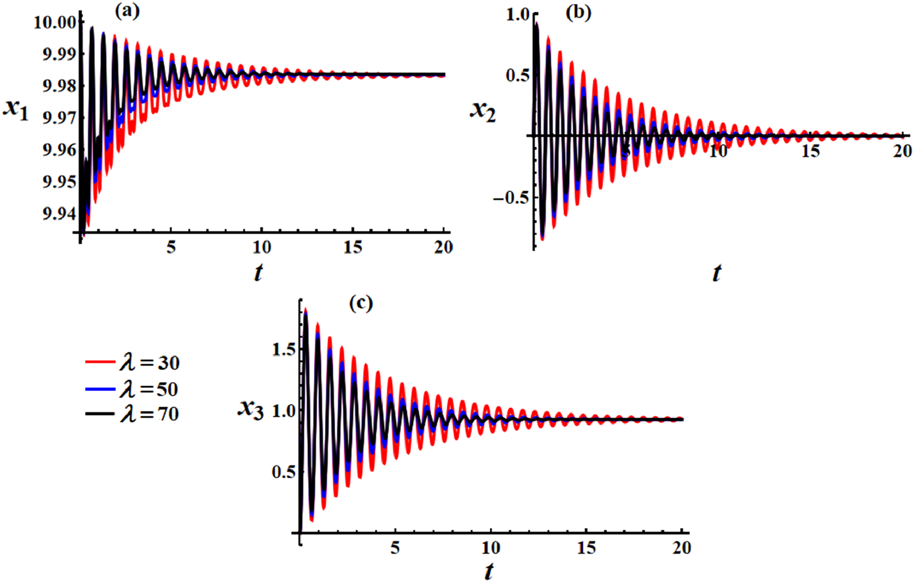
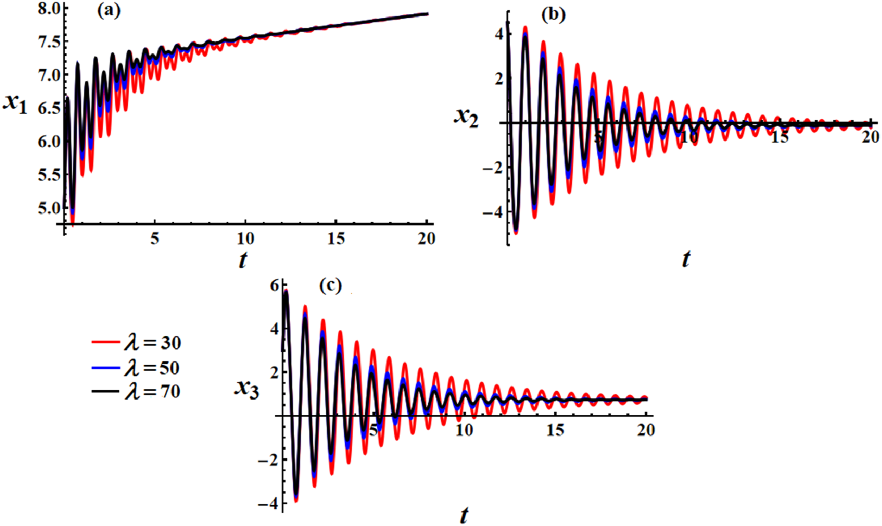
Figure (2) consists of three subplots, each showing the time evolution of the spacecraft’s angular velocities $x_1$ , $x_2$ , and $x_3$ , affected by different values of viscosity $\lambda =\left(30,50,70\right)\mathrm{N}.\mathrm{m}.\mathrm{s}$ in a viscid layer. Figure 2(a) shows a linear increase of $x_1$ overtime, with a very small oscillation at the beginning for lower time values. The effect of varying viscosity $\lambda$ is minimal on $x_1$ . The three curves for the different viscosities appear nearly identical after the initial small oscillation, which slightly dampens as $\lambda$ increases. This indicates that viscosity primarily affects initial transients but has little impact on long-term behavior for $x_1$ . In Figure 2(b), the angular velocity $x_2$ oscillates, showing damped oscillations that gradually die out over time. The red curve at $\lambda =30\mathrm{N}.\mathrm{m}.\mathrm{s}$ shows the least damping, with larger oscillations persisting for a longer time. As viscosity increases (blue curve at $\lambda =50\mathrm{N}.\mathrm{m}.\mathrm{s}$ ; black curve at $\lambda =70\mathrm{N}.\mathrm{m}.\mathrm{s}$ ), the oscillations dampen more rapidly. The higher the viscosity, the quicker the oscillations settle down to zero. This indicates that higher viscosity leads to faster energy dissipation and a quicker decay in the oscillations of $x_2$ . In Figure 2(c), the angular velocity $x_3$ also shows oscillatory behavior, similar to $x_2$ , but with a different amplitude and frequency. The damping effect of viscosity is evident here as well. The red curve at $\lambda =30\mathrm{N}.\mathrm{m}.\mathrm{s}$ oscillates with the least damping, while the blue at $\lambda =50\mathrm{N}.\mathrm{m}.\mathrm{s}$ and black at $\lambda =70\mathrm{N}.\mathrm{m}.\mathrm{s}$ curves show progressively faster damping. Similar to $x_2$ , higher viscosity accelerates the dissipation of the oscillations in $x_3$ .

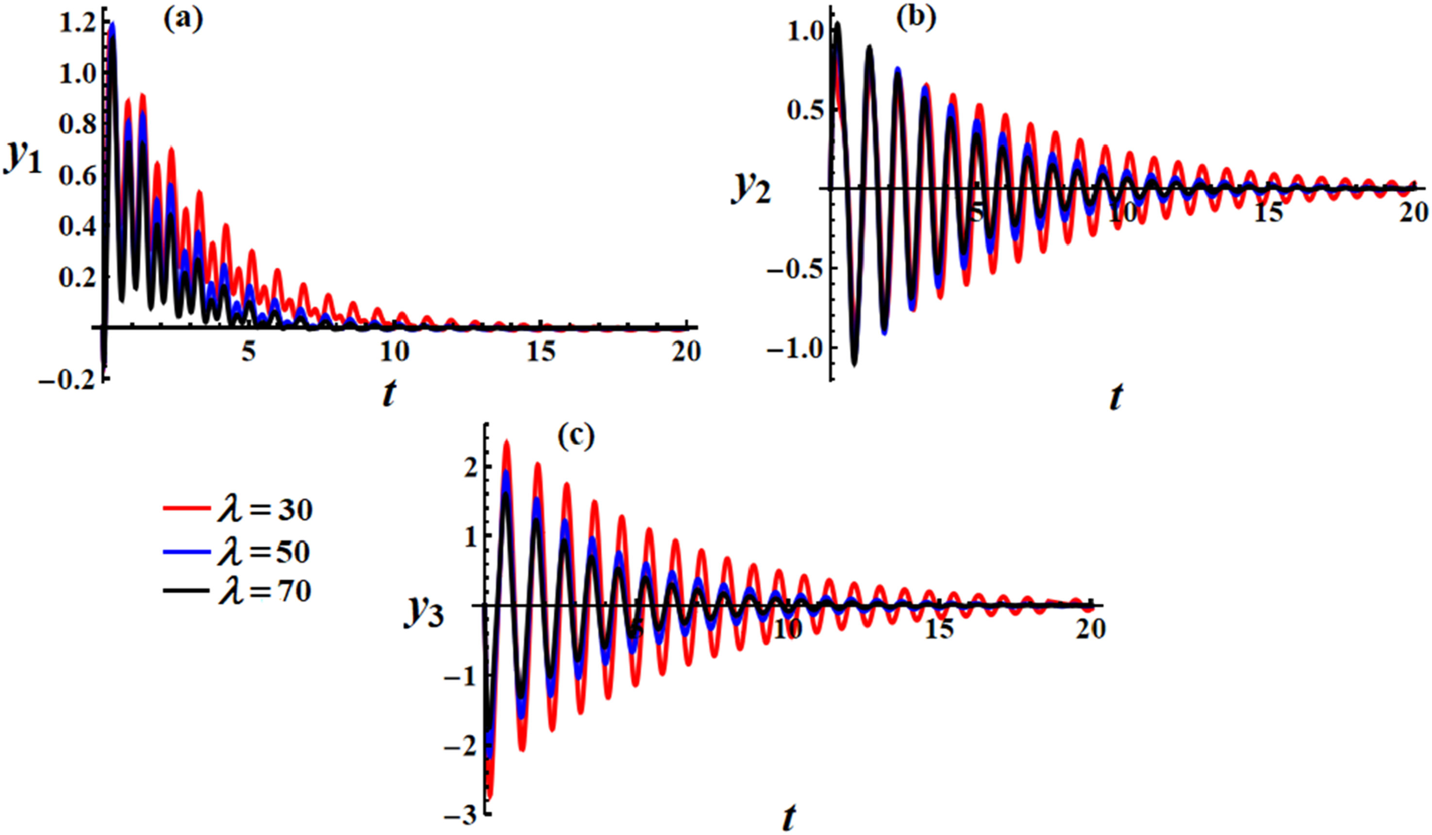
Figure 3 illustrates the time evolution of the slug’s angular velocities $y_1$ , $y_2$ , and $y_3$ , corresponding to different values of viscosity $\lambda =\left(30,50,70\right)\mathrm{N}.\mathrm{m}.\mathrm{s}$ . In Figure 3(a), the angular velocity $y_1$ begins with damped oscillations that quickly decay to zero, reaching near equilibrium at around $t=10$ . For the red curve at $\lambda =30\mathrm{N}.\mathrm{m}.\mathrm{s}$ , the oscillations persist slightly longer, while the blue curve at $\lambda =50\mathrm{N}.\mathrm{m}.\mathrm{s}$ and black curve at $\lambda =70\mathrm{N}.\mathrm{m}.\mathrm{s}$ show more rapid damping. As viscosity increases, the system’s resistance to motion is greater, leading to faster stabilization of $y_1$ . Higher viscosities damp the oscillations more quickly, and by $t=10$ , all values settle near zero. In Figure 3(b), the graph shows oscillatory behavior that gradually decays over time. The oscillations are symmetrical around zero value. The red curve at $\lambda =30\mathrm{N}.\mathrm{m}.\mathrm{s}$ exhibits the slowest decay, with oscillations lasting longer. The blue curve at $\lambda =50\mathrm{N}.\mathrm{m}.\mathrm{s}$ and black curve at $\lambda =70\mathrm{N}.\mathrm{m}.\mathrm{s}$ show progressively faster damping. As viscosity increases, oscillations die out more rapidly. Similar to $y_1$ , higher viscosity leads to faster energy dissipation and quicker stabilization of $y_2$ . In Figure 3(c), the angular velocity $y_3$ demonstrates larger oscillations compared to $y_1$ and $y_2$ , but it also exhibits damped oscillatory behavior. The red curve at $\lambda =30\mathrm{N}.\mathrm{m}.\mathrm{s}$ has the least damping, while the blue curve at $\lambda =50\mathrm{N}.\mathrm{m}.\mathrm{s}$ and black curve at $\lambda =70\mathrm{N}.\mathrm{m}.\mathrm{s}$ exhibit faster decay in the oscillations. Once again, higher viscosity leads to quicker damping of oscillations. The black curve shows the most rapid approach to equilibrium compared to the other values of viscosity. The impact of viscosity is clearly visible in the damping behavior, with larger viscosity resulting in the fastest stabilization of all angular velocities.

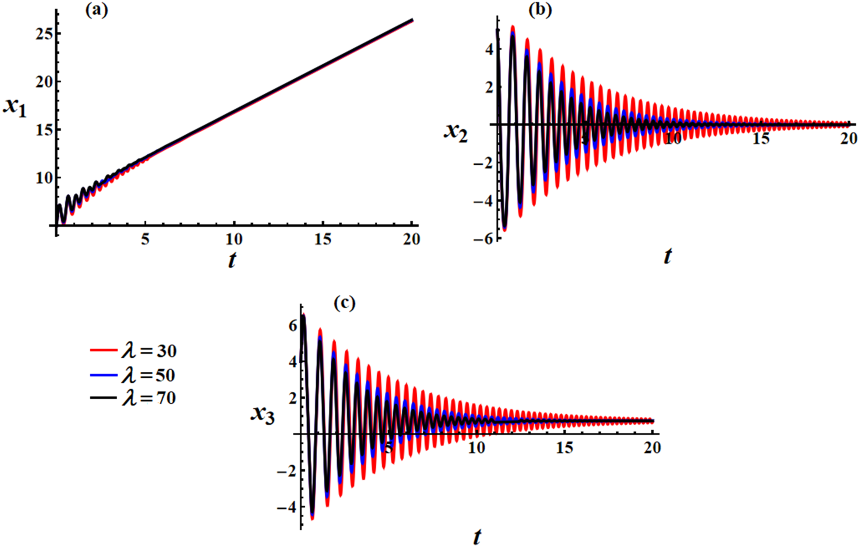
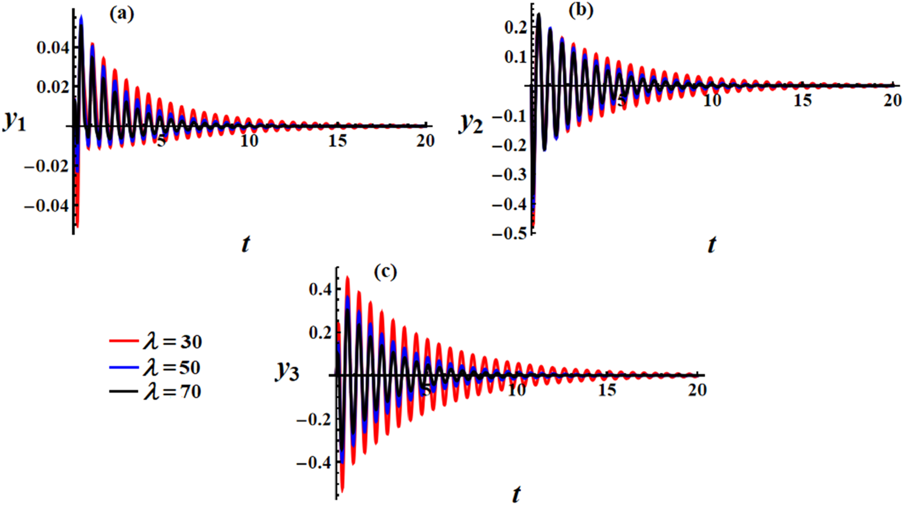
Figure (4) shows the time evolution of the spacecraft’s angular velocities $x_1$ , $x_2$ , and $x_3$ , corresponding to different values of the GM ${\mathcal{l}}_3=\left(100,300,500\right)\text{kg}.{\mathrm{m}}^2.{\mathrm{s}}^{‐1}$ . In Figure 4(a), the angular velocity $x_1$ increases almost linearly with time, indicating that the spacecraft undergoes continuous rotation around the major axis as time progresses. There is slight oscillation at the beginning, which quickly damps out. This oscillation corresponds to the interplay between the torque and the GM, as well as the dissipative effects of the system. The initial oscillations are more pronounced for lower values of ${\mathcal{l}}_3$ (the red curve, where ${\mathcal{l}}_3=100\text{kg}.{\mathrm{m}}^2.{\mathrm{s}}^{‐1}$ ). As ${\mathcal{l}}_3$ increases, the oscillations become smaller (blue curve for ${\mathcal{l}}_3=300\text{kg}.{\mathrm{m}}^2.{\mathrm{s}}^{‐1}$ ) and almost disappear for ${\mathcal{l}}_3=500\text{kg}.{\mathrm{m}}^2.{\mathrm{s}}^{‐1}$ (black curve), which suggests that higher GMs reduce the amplitude of initial oscillations, leading to more stable rotation over time. In Figure 4(b), the angular velocity $x_2$ (about the second axis) exhibits a decaying oscillation, meaning that the spacecraft experiences a wobbling motion initially but stabilizes as time progresses. This damped oscillation suggests energy dissipation in the system, likely due to the viscid layer around the slug. The oscillation amplitude is largest for the red curve ( ${\mathcal{l}}_3=100\text{kg}.{\mathrm{m}}^2.{\mathrm{s}}^{‐1}$ ) and gradually reduces for the blue and black curves. This indicates that increasing ${\mathcal{l}}_3$ leads to faster damping of the oscillations, contributing to stability. The oscillations decay over time, but at different rates depending on the value of ${\mathcal{l}}_3$ . Larger values of ${\mathcal{l}}_3$ (the black curve) result in quicker damping, which stabilizes the spacecraft’s motion more effectively. In Figure 4(c), Similar to $x_2$ , the angular velocity $x_3$ shows oscillations that gradually decay. However, the behavior is more complex, with initial amplitudes varying significantly for different ${\mathcal{l}}_3$ values. For lower ${\mathcal{l}}_3$ values (red curve), the oscillations have a larger amplitude and decay more slowly. As ${\mathcal{l}}_3$ increases (blue and black curves), the oscillations become smaller and damp out faster. This again highlights that larger GMs stabilize the spacecraft more efficiently. The curves converge to different final oscillation amplitudes depending on ${\mathcal{l}}_3$ . The higher the GM (black curve), the higher the stabilized amplitude, showing that a stronger GM affects the spacecraft’s long-term behavior after dissipation. In the long run, all plots show stabilization, with the spacecraft angular velocities converging to steady values, especially in $x_1$ . This reflects a situation where the spacecraft reaches a stable rotational state due to the dissipative effects of the viscid layer and the stabilizing influence of the GM.

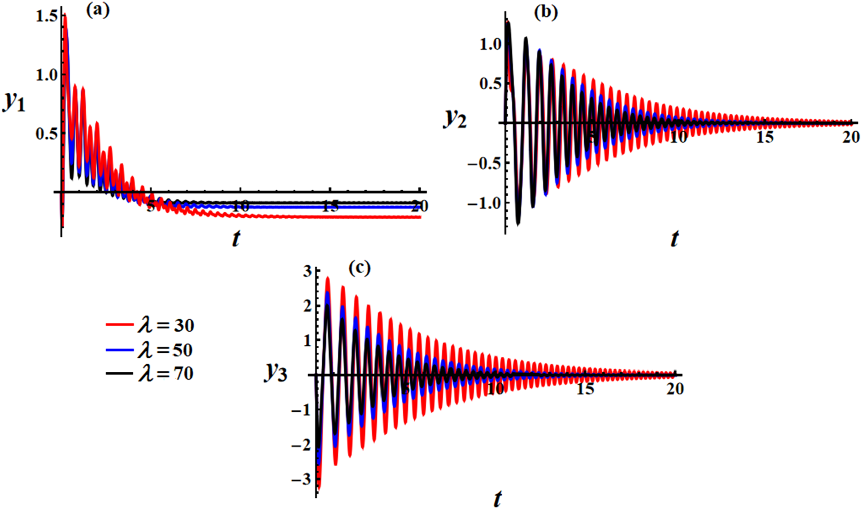
Figure (5) presents the time evolution of the slug angular velocities $y_1$ , $y_2$ , and $y_3$ , corresponding to different values of the GM ${\mathcal{l}}_3=\left(100,300,500\right)\text{kg}.{\mathrm{m}}^2.{\mathrm{s}}^{‐1}$ . In Figure 5(a), the angular velocity $y_1$ shows significant oscillations at the beginning, which are highly damp as time progresses, which indicates that the slug initially responds strongly to the applied torque but quickly stabilizes due to the energy dissipation effects of the viscid layer. The red curve at ${\mathcal{l}}_3=100\text{kg}.{\mathrm{m}}^2.{\mathrm{s}}^{‐1}$ shows the largest initial oscillations, while the black curve at ${\mathcal{l}}_3=500\text{kg}.{\mathrm{m}}^2.{\mathrm{s}}^{‐1}$ exhibits the smallest oscillation amplitude. As ${\mathcal{l}}_3$ increases, the damping effect is stronger, leading to a more stable behavior at earlier time stages. The amplitude decreases rapidly, approaching zero. By $t\approx 10$ , the angular velocity stabilizes, reaching near-zero values for all ${\mathcal{l}}_3$ , indicating that the slug’s motion about this axis has nearly ceased. In Figure 5(b), the angular velocity $y_2$ shows oscillations that persist for a longer time compared to $y_1$ . Although the oscillations decay over time, they do so more slowly. This suggests that the slug continues to oscillate for an extended period before the energy dissipates completely. Similar to $y_1$ , the red curve at ${\mathcal{l}}_3=100\text{kg}.{\mathrm{m}}^2.{\mathrm{s}}^{‐1}$ shows the largest oscillation amplitude, and the black curve at ${\mathcal{l}}_3=500\text{kg}.{\mathrm{m}}^2.{\mathrm{s}}^{‐1}$ shows the smallest. However, the differences between the curves are less pronounced here, suggesting that ${\mathcal{l}}_3$ has a milder effect on damping for $y_2$ compared to $y_1$ . Around $t=20$ , the oscillations diminish significantly for all values of ${\mathcal{l}}_3$ , with larger GM leading to faster damping. In Figure 5(c), the angular velocity $y_3$ exhibits oscillations similar to $y_2$ , but with larger initial amplitudes. Oscillations also decay over time, though at a slower rate compared to $y_1$ . As in the other cases, increasing ${\mathcal{l}}_3$ reduces the initial amplitude and hastens the damping of oscillations. The red curve at ${\mathcal{l}}_3=100\text{kg}.{\mathrm{m}}^2.{\mathrm{s}}^{‐1}$ shows the largest oscillation amplitude, while the black curve at ${\mathcal{l}}_3=500\text{kg}.{\mathrm{m}}^2.{\mathrm{s}}^{‐1}$ shows the smallest. The stronger damp with larger ${\mathcal{l}}_3$ values is again apparent. By $t\approx 20$ , the slug’s motion about this axis has significantly diminished, although the black curve still shows minor residual oscillations. All components of the slug’s angular velocity eventually stabilize, with oscillations damping out entirely by $t=20$ . This shows that the spacecraft’s internal slug motion ceases over time, contributing to the overall stability of the system.

For minor axis torque

In this scenario, we investigate spacecraft motion under the assumption that the torque along the minor axis is constant. Figures (6)–(9) are plotted at $\left(M_1,M_2,M_3\right)=\left(0,0,10\right)\mathrm{N}.\mathrm{m}$ inside an interval $\tau \in \left[0,20\right]s$ .

In Figure (6), we analyze the evolution of the angular velocities $x_1$ , $x_2$ , and $x_3$ of the spacecraft considering different values of the viscosity parameter $\lambda$ in the viscid layer surrounding the slug. In Figure 6(a), the angular velocity $x_1$ starts with rapid oscillations, gradually stabilizing and showing a monotonic increase after an initial transient phase. The initial oscillations arise due to the interaction between the torque and the rotational inertia of the rigid body. Over time, as the viscosity increases (red: $\lambda =30\mathrm{N}.\mathrm{m}.\mathrm{s}$ , blue: $\lambda =50\mathrm{N}.\mathrm{m}.\mathrm{s}$ , black: $\lambda =70\mathrm{N}.\mathrm{m}.\mathrm{s}$ ), the oscillations damp out more effectively, with higher viscosity leading to faster stabilization. The curves reveal that increased viscosity suppresses oscillations more quickly. As $\lambda$ increases from 30 (red) to 70 (black), the oscillatory behavior decays faster, and the system settles to a steady-state linear growth earlier. After about $t=15$ , the system approaches a quasi-linear regime where $x_1$ grows steadily, with minimal oscillatory disturbances. In Figure 6(b), the angular velocity $x_2$ exhibits oscillatory behavior around zero, with the amplitude of oscillations diminishing over time. The oscillations in $x_2$ represent the exchange of angular momentum between different rotational components of the system. The damping effect is visibly controlled by the viscosity parameter $\lambda$ . For lower viscosity (red: $\lambda =30\mathrm{N}.\mathrm{m}.\mathrm{s}$ ), the oscillations are more pronounced and take longer to decay. As the viscosity increases (blue: $\lambda =50\mathrm{N}.\mathrm{m}.\mathrm{s}$ , black: $\lambda =70\mathrm{N}.\mathrm{m}.\mathrm{s}$ ), the amplitude of oscillations reduces more quickly, highlighting the energy dissipation induced by higher viscosity. Around $t=15$ , the system approaches a near-steady state, where oscillations are nearly negligible, especially for higher-viscosity values. Similar to $x_2$ , the angular velocity $x_3$ exhibits strong oscillations initially, which gradually decrease in amplitude over time. This plot reflects the behavior of the spacecraft angular velocity along the third axis. The dampening of oscillations occurs as energy dissipates due to the interaction between the body torque and the viscous layer surrounding the slug. The amplitude of oscillations decays more rapidly as viscosity increases. The red curve ( $\lambda =30\mathrm{N}.\mathrm{m}.\mathrm{s}$ ) displays persistent oscillations, while the black curve ( $\lambda =70\mathrm{N}.\mathrm{m}.\mathrm{s}$ ) shows a much faster decay, illustrating the role of viscosity in energy dissipation. After about $t=15$ , the oscillations become minimal, indicating that the system has entered a damped, low-energy state where angular velocity $x_3$ fluctuates around a nearly constant value.

In Figure (7), three subplots (a), (b), and (c) show the time evolution of the slug’s angular velocity components $y_1$ , $y_2$ , and $y_3$ under different values of the viscosity parameter $\lambda$ in the viscid layer. The black, blue, and red curves correspond to $\lambda =70\mathrm{N}.\mathrm{m}.\mathrm{s}$ , $\lambda =50\mathrm{N}.\mathrm{m}.\mathrm{s}$ , and $\lambda =30\mathrm{N}.\mathrm{m}.\mathrm{s}$ , respectively. In Figure 7(a), the graph starts with an initial peak close to 1.2, showing a rapid decay overtime. At $\lambda =70\mathrm{N}.\mathrm{m}.\mathrm{s}$ , the oscillations decay quickly, with significant damping present early on. However, at $\lambda =30\mathrm{N}.\mathrm{m}.\mathrm{s}$ , the oscillations persist for a longer period before damping out, showing that lower viscosity allows the angular velocity to oscillate more freely before being dissipated. The amplitude of oscillations decreases as time progresses and after around $t=10$ , all curves show minimal oscillation. In Figure 7(b), the plot for $y_2$ displays a clear oscillatory pattern similar to $y_1$ , but with symmetric oscillations around zero. At $\lambda =70\mathrm{N}.\mathrm{m}.\mathrm{s}$ , the oscillations decay faster, and the black curve quickly converges to a near-zero amplitude, but at $\lambda =30\mathrm{N}.\mathrm{m}.\mathrm{s}$ , the red curve shows sustained oscillations with larger amplitude, and the decay is slower compared to the higher-viscosity cases. The damping effect is evident in all three curves, with lower viscosity allowing for higher oscillation amplitudes. In Figure 7(c), this plot has a slightly different behavior compared to the other two, starting with a higher amplitude oscillation (about 2.5) that decays over time. For $\lambda =70\mathrm{N}.\mathrm{m}.\mathrm{s}$ , as with the other components, the black curve decays the quickest. For $\lambda =30\mathrm{N}.\mathrm{m}.\mathrm{s}$ , the red curve sustains oscillations for a longer time, showing that viscosity plays a critical role in determining how quickly the oscillations die down. The damping is more gradual for the red curve, while the black curve converges to zero faster.

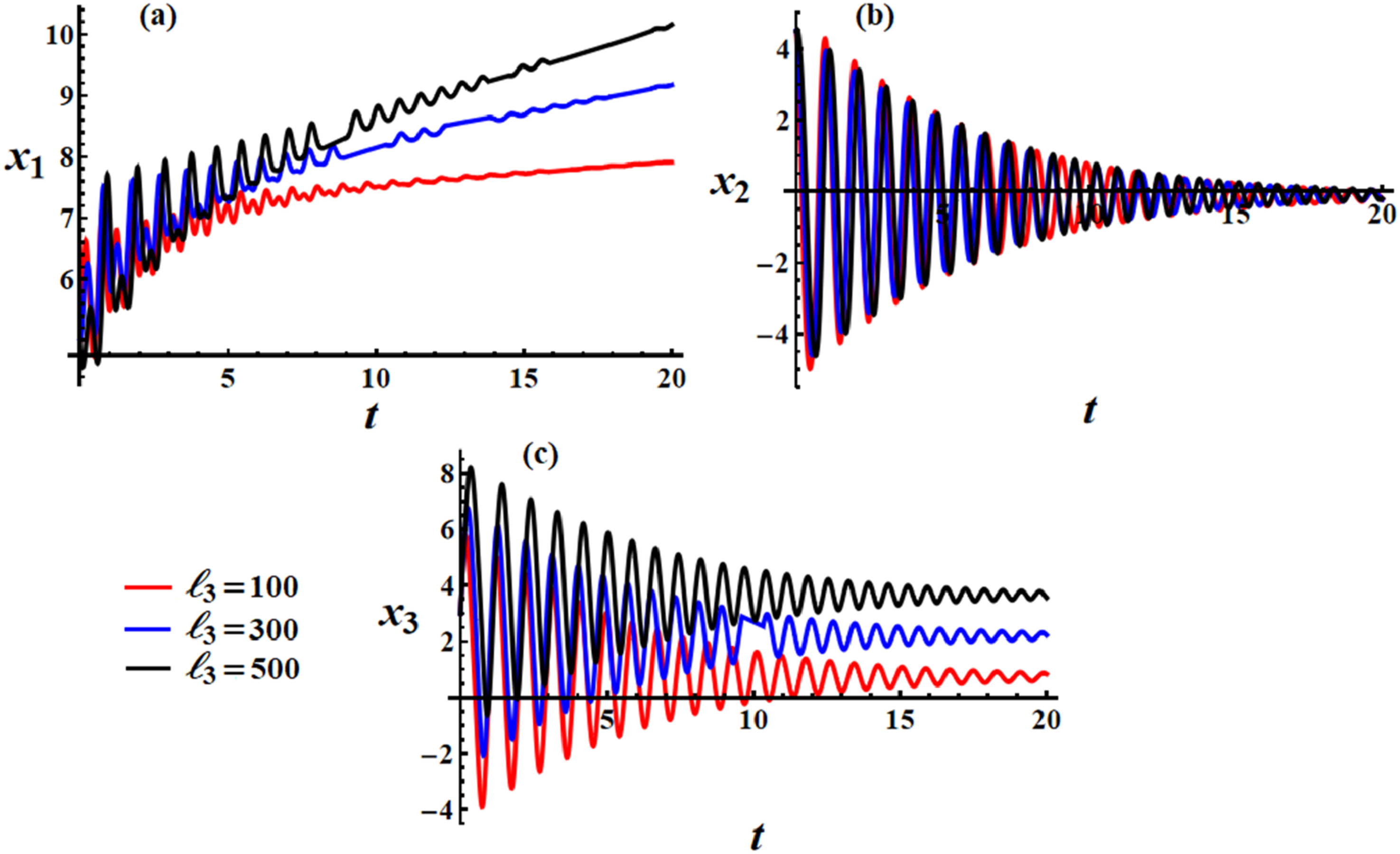
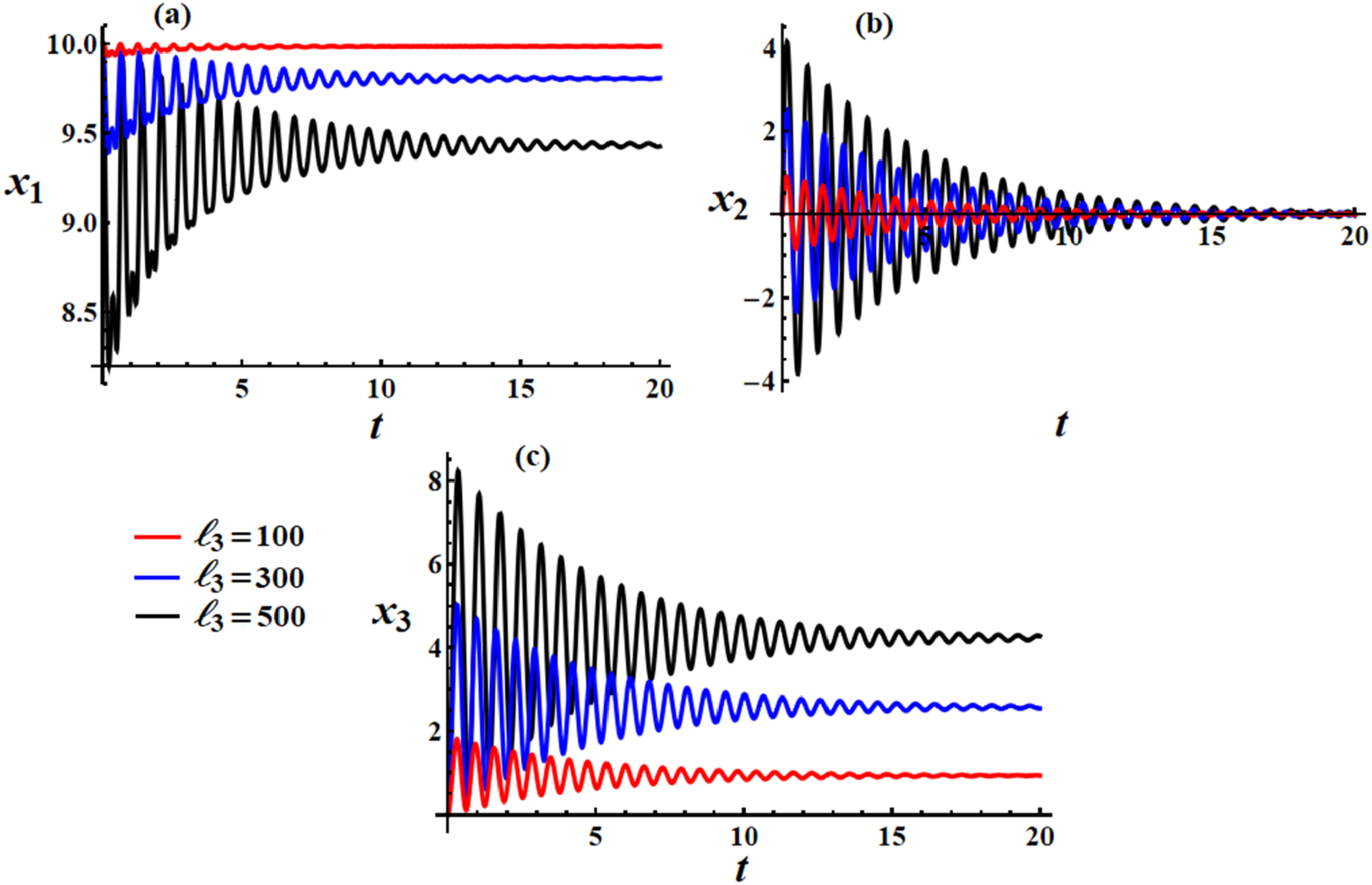
Figure (8) analyzes the angular velocities $x_1$ , $x_2$ , and $x_3$ of the spacecraft for the minor axis constant torque case correspond to various values of the GM ${\mathcal{l}}_3$ . In Figure 8(a), the angular velocity $x_1$ grows over time, but with significant oscillations superimposed on this growth. This oscillatory behavior is indicative of complex interactions between the applied torque, the inertial properties of the spacecraft, and the internal dynamics of the system. For smaller ${\mathcal{l}}_3$ (red, ${\mathcal{l}}_3=100\text{kg}.{\mathrm{m}}^2.{\mathrm{s}}^{‐1}$ ), the growth is slower, and the oscillations are more subdued. As ${\mathcal{l}}_3$ increases (blue for ${\mathcal{l}}_3=300\text{kg}.{\mathrm{m}}^2.{\mathrm{s}}^{‐1}$ and black for ${\mathcal{l}}_3=500\text{kg}.{\mathrm{m}}^2.{\mathrm{s}}^{‐1}$ ), the rate of growth of $x_1$ increases and the amplitude of oscillations also becomes more pronounced. The largest oscillations and fastest growth are seen in the black curve at ${\mathcal{l}}_3=500\text{kg}.{\mathrm{m}}^2.{\mathrm{s}}^{‐1}$ , indicating that a higher GM increases the rotational inertia and the system’s dynamic response. Over time, the amplitude of the oscillations decreases slightly but not entirely, suggesting that energy dissipation has a partial damping effect on these oscillations. In Figure 8(b), the angular velocity $x_2$ exhibits clear oscillations that decay over time, indicating a damped response in this direction. The oscillations are initially large but gradually reduce in amplitude as time progresses, showing the dissipative nature of the system. For ${\mathcal{l}}_3=100\text{kg}.{\mathrm{m}}^2.{\mathrm{s}}^{‐1}$ , the oscillations have a relatively smaller amplitude and decay more quickly. As ${\mathcal{l}}_3$ increases, the amplitude of the oscillations also increases, and the damping is slower, with the black curve ( ${\mathcal{l}}_3=500\text{kg}.{\mathrm{m}}^2.{\mathrm{s}}^{‐1}$ ) showing the largest oscillation amplitude and slowest decay, which implies that higher GM reduces the rate of energy dissipation, resulting in sustained oscillatory behavior. By $t=20$ , the oscillations have nearly died out for all curves, with the system reaching a near-stable state for all ${\mathcal{l}}_3$ . In Figure 8(c), the angular velocity $x_3$ shows oscillations with varying amplitude depending on ${\mathcal{l}}_3$ . The black curve maintains the largest amplitude oscillations, while the red shows the smallest oscillations. The frequency of oscillations is relatively high for all curves, but the amplitude decreases as $t$ increases. The system exhibits a more gradual damping of the oscillations for the larger GM at ${\mathcal{l}}_3=500\text{kg}.{\mathrm{m}}^2.{\mathrm{s}}^{‐1}$ , while the red curve at ${\mathcal{l}}_3=100\text{kg}.{\mathrm{m}}^2.{\mathrm{s}}^{‐1}$ damps more quickly. After $t\approx 10$ , the system stabilizes, with oscillations persisting only in the larger ${\mathcal{l}}_3$ cases (black curve). The red and blue curves show much smaller oscillations by this time.

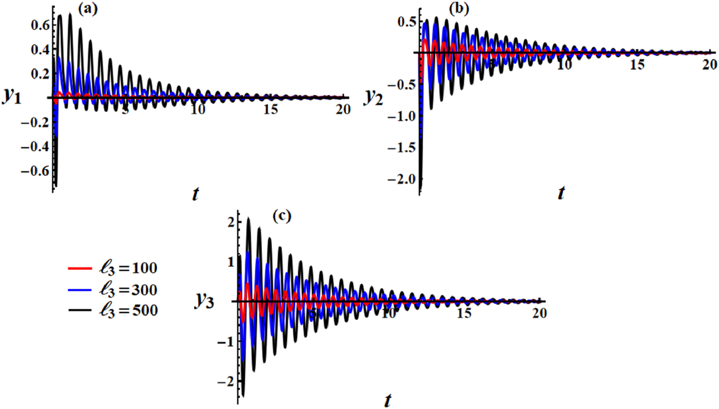
Figure (9) examines the slug angular velocities $y_1$ , $y_2$ , and $y_3$ for the minor axis constant torque case, focusing on the slug’s behavior under different values of the GM ${\mathcal{l}}_3$ . In Figure 9(a), the $y_1$ component starts with relatively large oscillations, which gradually decrease in amplitude over time, which represents a typical damped oscillatory response. For smaller ${\mathcal{l}}_3$ values (red, ${\mathcal{l}}_3=100\text{kg}.{\mathrm{m}}^2.{\mathrm{s}}^{‐1}$ ), the damping occurs more quickly, and the oscillations are less pronounced. As ${\mathcal{l}}_3$ increases, the amplitude of the oscillations grows larger, and the damping is slower. The black curve ( ${\mathcal{l}}_3=500\text{kg}.{\mathrm{m}}^2.{\mathrm{s}}^{‐1}$ ) shows the most pronounced oscillations with the slowest decay rate. This behavior indicates that larger GM causes a more sustained oscillatory response in the slug’s angular velocity in the $y_1$ direction. By $t\approx 10$ , the oscillations have mostly dissipated, and the system stabilizes to a nearly zero value for $y_1$ . In Figure 9(b), the $y_2$ component behaves similarly to $y_1$ , showing damped oscillations. However, the oscillations are smaller in magnitude and are centered closer to zero. Smaller ${\mathcal{l}}_3$ values (red curve) show faster damping, while larger ${\mathcal{l}}_3$ values (black curve) exhibit sustained oscillations. The amplitude of oscillations is smaller for all curves compared to $y_1$ , indicating less dynamic motion in the $y_2$ direction. By $t\approx 15$ , the oscillations become minimal for all values of ${\mathcal{l}}_3$ , with near-zero velocity for $y_2$ . In Figure 9(c), the $y_3$ component shows the most persistent oscillations, especially for the larger ${\mathcal{l}}_3$ values. Even at $t\approx 20$ , the black curve at ${\mathcal{l}}_3=500\text{kg}.{\mathrm{m}}^2.{\mathrm{s}}^{‐1}$ still exhibits some oscillations. For smaller ${\mathcal{l}}_3$ (red curve), the oscillations damp more quickly, but as ${\mathcal{l}}_3$ increases, the amplitude and persistence of the oscillations grow. The black curve shows the slowest damping, while the red curve stabilizes the fastest, indicating a strong correlation between the GM and the persistence of oscillations in the $y_3$ direction. For all values of ${\mathcal{l}}_3$ , the system shows stabilization in the $y_3$ direction by $t=20$ , though some oscillations remain for the black curve. By $t\approx 20$ , all components have nearly stabilized, with minimal oscillations remaining. The $y_1$ and $y_2$ components show near-zero velocities, while $y_3$ exhibits small residual oscillations for higher ${\mathcal{l}}_3$ values.

For intermediate axis torque

In this scenario, we investigate the spacecraft motion under the assumption that the torque along the intermediate axis is constant. Figures (10)–(13) are plotted at $\left(M_1,M_2,M_3\right)=\left(0,10,0\right)\mathrm{N}.\mathrm{m}$ inside an interval $\tau \in \left[0,20\right]s$ .

Figure (10) represents the evolution of the angular velocities $x_1$ , $x_2$ , and $x_3$ of the spacecraft over time under the influence of various values of the layer viscosity parameter. In Figure 10(a), the graph shows that $x_1$ experiences an initial rapid increase, followed by damped oscillations. These oscillations reduce overtime, indicating the influence of viscosity in dissipating energy. As $\lambda$ increases, the damping effect becomes more pronounced, resulting in fewer and smaller oscillations for larger viscosity values. After the oscillatory period, all curves exhibit steady linear growth, reflecting that the system is stabilizing after the energy dissipation caused by the viscosity. In Figure 10(b), for $x_2$ , the angular velocity initially oscillates between positive and negative values, with the oscillations diminishing over time. This behavior demonstrates how viscosity opposes and reduces oscillatory motion. The black curve ( $\lambda =70\mathrm{N}.\mathrm{m}.\mathrm{s}$ ) shows the fastest damping, indicating that higher viscosity suppresses oscillations more effectively. The system reaches a near-zero steady state after approximately $t=15$ , with the oscillations becoming negligible, showing that the intermediate axis torque and viscosity work together to stabilize $x_2$ . In Figure 10(c), similar to $x_2$ , $x_3$ undergoes damped oscillations, with the damping effect being stronger for larger viscosity values. The oscillations are more pronounced at earlier times, but for larger $\lambda$ , the motion quickly dampens. By $t\approx 10$ , the oscillations become minimal, and the system stabilizes. The black curve shows the most significant damping, while the red curve exhibits more prolonged oscillations due to the lower viscosity value.

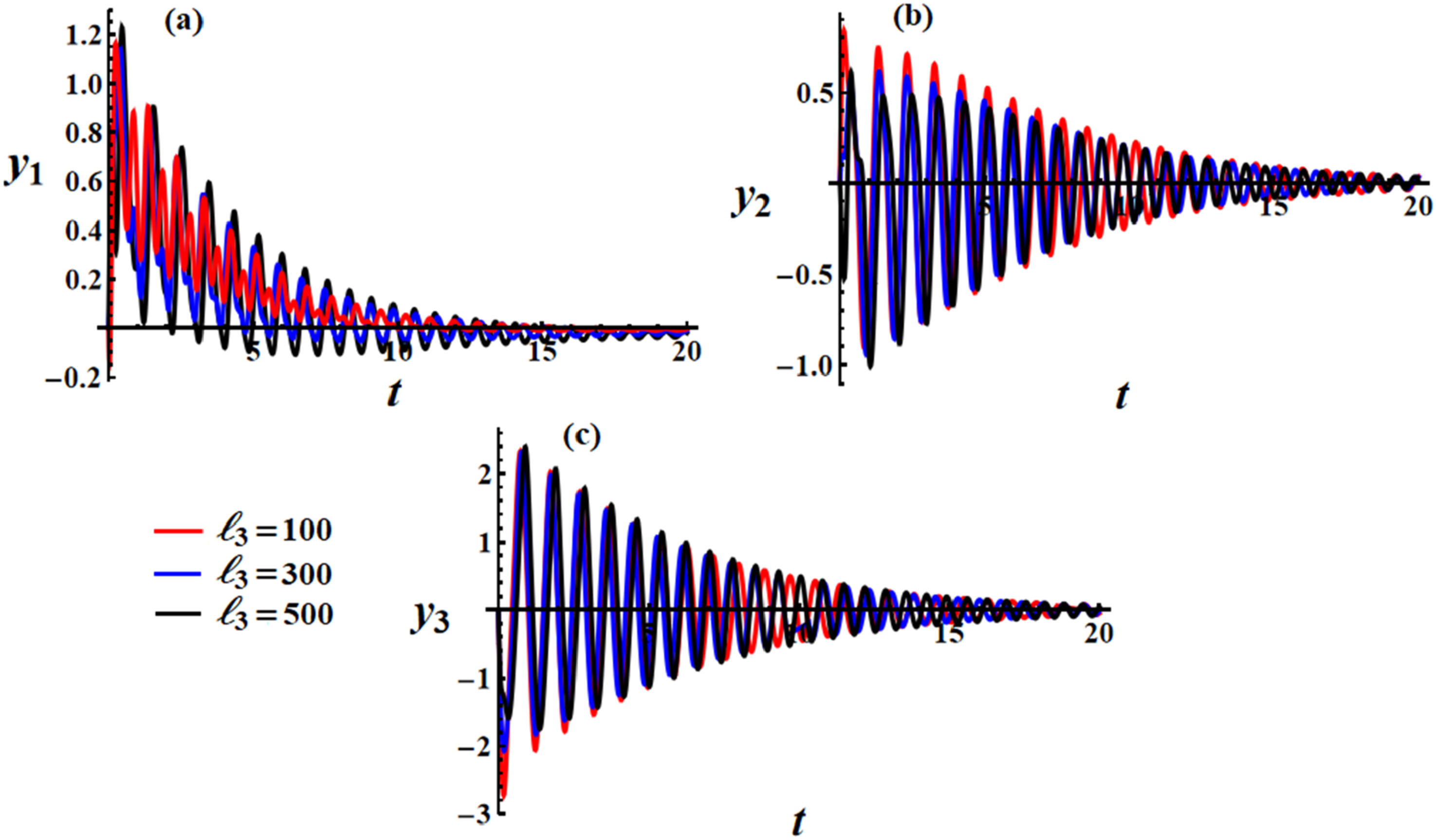
Figure (11) represents the time evolution of the slug’s angular velocities $y_1$ , $y_2$ , and $y_3$ under the influence of varying viscosity values. In Figure 11(a), the graph shows that $y_1$ undergoes rapid oscillations with a significant initial amplitude, which is damped over time. The damping rate increases with higher-viscosity values ( $\lambda =70\mathrm{N}.\mathrm{m}.\mathrm{s}$ shows the quickest decay). Lower viscosity ( $\lambda =30\mathrm{N}.\mathrm{m}.\mathrm{s}$ ) results in prolonged oscillations. After $t=10$ , the angular velocity effectively stabilizes around zero, reflecting the damping of rotational motion in the slug due to energy dissipation. In Figure 11(b), similar to $y_1$ , $y_2$ exhibits oscillations that are damped more quickly for higher viscosity. Initially, $y_2$ oscillates symmetrically around zero, with the black curve ( $\lambda =70\mathrm{N}.\mathrm{m}.\mathrm{s}$ ) showing the fastest suppression of oscillations. By $t\approx 15$ , the oscillations become minimal for all values of $\lambda$ , demonstrating that the slug angular velocity $y_2$ stabilizes more rapidly in higher-viscosity environments. In Figure 11(c), the angular velocity $y_3$ starts with larger oscillations compared to $y_1$ and $y_2$ , with the amplitude of oscillation diminishing over time. As with the previous graphs, higher viscosity ( $\lambda =70\mathrm{N}.\mathrm{m}.\mathrm{s}$ ) leads to faster damping. The system stabilizes after $t=15$ , with the oscillations being significantly reduced for all values of viscosity.

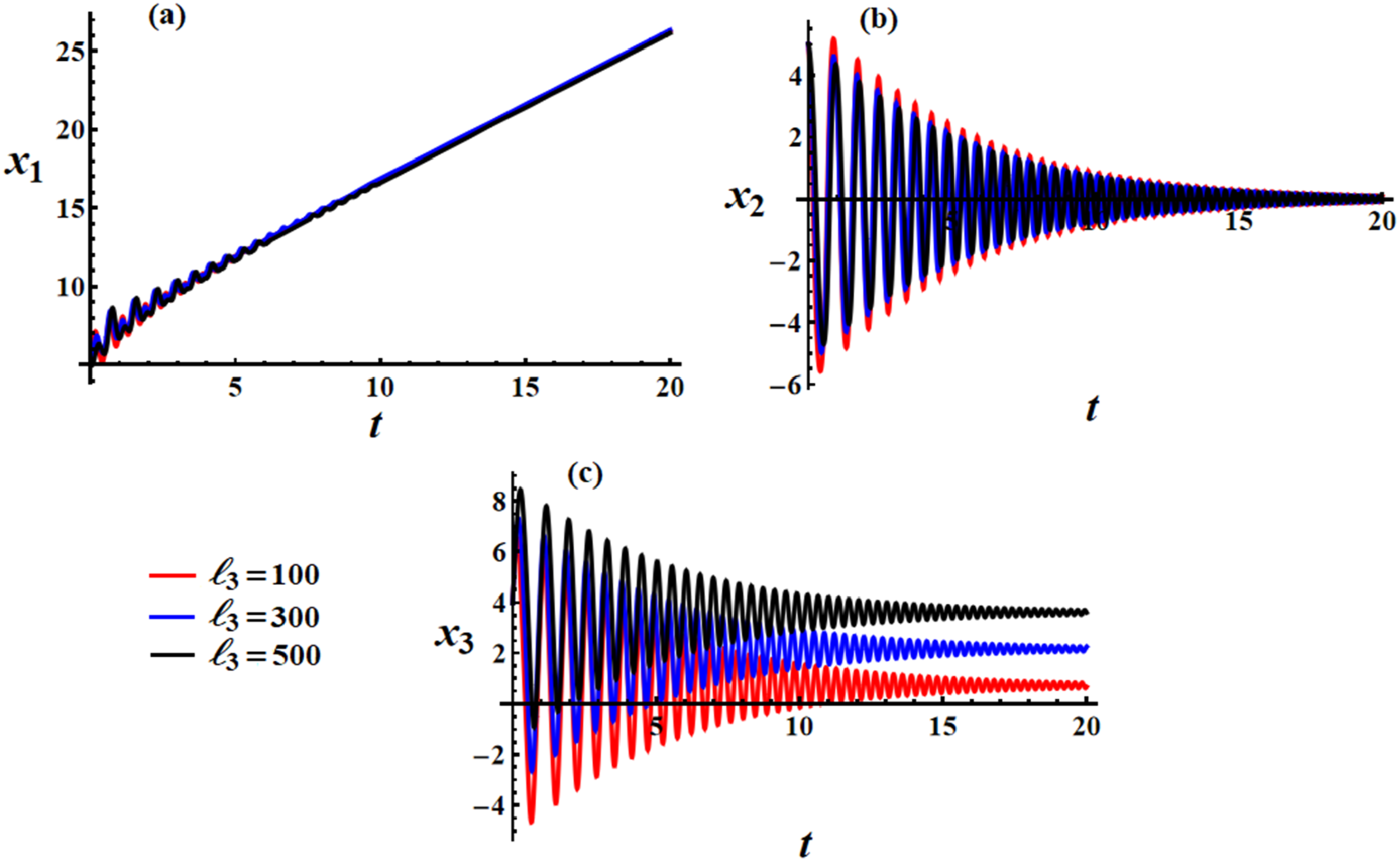
Figure (12) illustrates the behavior of the spacecraft angular velocities $x_1$ , $x_2$ , and $x_3$ under intermediate axis’ constant torque conditions correspond to different values of the GM ${\mathcal{l}}_3$ . In Figure 12(a), initially at ${\mathcal{l}}_3=100\text{kg}.{\mathrm{m}}^2.{\mathrm{s}}^{‐1}$ , $x_1$ undergoes small oscillations but stabilizes around $x_1=10$ over time. The oscillations decay quickly, indicating strong damping effects, potentially due to low gyrostatic effects. With a higher GM ${\mathcal{l}}_3=300\text{kg}.{\mathrm{m}}^2.{\mathrm{s}}^{‐1}$ , the oscillations in $x_1$ are larger initially and persist for a longer duration. However, the curve stabilizes $x_1=9.7$ after a longer period compared to ${\mathcal{l}}_3=100\text{kg}.{\mathrm{m}}^2.{\mathrm{s}}^{‐1}$ . The black curve at ${\mathcal{l}}_3=500\text{kg}.{\mathrm{m}}^2.{\mathrm{s}}^{‐1}$ shows the most significant oscillations. It stabilizes to a lower value around $x_1=9$ , but the damping is weaker, and the oscillations persist longer, demonstrating that increasing ${\mathcal{l}}_3$ intensifies the oscillatory behavior. In Figure 12(b), for ${\mathcal{l}}_3=100\text{kg}.{\mathrm{m}}^2.{\mathrm{s}}^{‐1}$ , the oscillations are damped quickly, and $x_2$ returns to nearly zero around $t=10$ . For ${\mathcal{l}}_3=300\text{kg}.{\mathrm{m}}^2.{\mathrm{s}}^{‐1}$ , the oscillations are larger, and the damping is slower compared to the red curve. The curve starts to stabilize at $t=15$ . For ${\mathcal{l}}_3=500\text{kg}.{\mathrm{m}}^2.{\mathrm{s}}^{‐1}$ , the most significant oscillations occur, and damping is even slower, showing that the GM ${\mathcal{l}}_3$ significantly affects the persistence of the oscillations. In Figure 12(c), at ${\mathcal{l}}_3=100\text{kg}.{\mathrm{m}}^2.{\mathrm{s}}^{‐1}$ , the oscillations damp quickly, and $x_3$ stabilizes at approximately $x_3=2$ , indicating a smaller influence of ${\mathcal{l}}_3$ . With blue curve at ${\mathcal{l}}_3=300\text{kg}.{\mathrm{m}}^2.{\mathrm{s}}^{‐1}$ , the oscillations are more pronounced and take longer to stabilize at a higher value, $x_3\approx 3.5$ , suggesting stronger gyrostatic influence. For the black curve at ${\mathcal{l}}_3=500\text{kg}.{\mathrm{m}}^2.{\mathrm{s}}^{‐1}$ , with the highest GM, the oscillations are significantly larger and persist throughout the duration, settling around $x_3=5$ . This shows that as ${\mathcal{l}}_3$ increases, the system experiences larger oscillations and takes longer to reach equilibrium. For $x_1$ and $x_3$ , higher values of ${\mathcal{l}}_3$ lead to lower final equilibrium points, with $x_1$ stabilizing lower and $x_3$ stabilizing higher as ${\mathcal{l}}_3$ increases. $x_2$ consistently tends to zero, but larger values of ${\mathcal{l}}_3$ prolong the time it takes to reach this state.

Figure (13) illustrates the behavior of the slug’s angular velocities $y_1$ , $y_2$ , and $y_3$ for the intermediate axis constant torque case, under the influence of different values of the GM ${\mathcal{l}}_3$ . In Figure 13(a), the angular velocity $y_1$ displays damped oscillations that decrease in amplitude as time progresses. The black curve ( ${\mathcal{l}}_3=500\text{kg}.{\mathrm{m}}^2.{\mathrm{s}}^{‐1}$ ) shows the largest amplitude and the slowest decay, while the red curve ( ${\mathcal{l}}_3=100\text{kg}.{\mathrm{m}}^2.{\mathrm{s}}^{‐1}$ ) displays the fastest decay and smallest amplitude. The system stabilizes more quickly for smaller values of ${\mathcal{l}}_3$ , while higher ${\mathcal{l}}_3$ values prolong the oscillations and delay stabilization. The oscillatory behavior reflects the coupling between the slug’s rotational dynamics and the spacecraft’s body, with the larger GM inducing more pronounced oscillations. The faster decay in the red curve suggests that the energy dissipation mechanisms dominate more effectively at lower GMs. In Figure 13(b), similar to $y_1$ , the angular velocity $y_2$ exhibits oscillatory motion, with the amplitude decreasing over time. The red curve ( ${\mathcal{l}}_3=100\text{kg}.{\mathrm{m}}^2.{\mathrm{s}}^{‐1}$ ) again shows a faster decay, while the black curve ( ${\mathcal{l}}_3=500\text{kg}.{\mathrm{m}}^2.{\mathrm{s}}^{‐1}$ ) oscillates with a higher amplitude and takes longer to decay. The $y_2$ dynamics mirror the behavior seen in $y_1$ , although the oscillations here are larger in magnitude. The $y_2$ behavior suggests that the slug’s response to the torque is influenced by the interplay between the GM and the slug’s internal dissipation. The larger the ${\mathcal{l}}_3$ , the more energy remains in the system for a longer time, sustaining oscillations. In Figure 13(c), the angular velocity $y_3$ starts with significant oscillations and gradually decays over time. As with $y_1$ and $y_2$ , the black curve ( ${\mathcal{l}}_3=500\text{kg}.{\mathrm{m}}^2.{\mathrm{s}}^{‐1}$ ) shows the highest amplitude and the slowest decay, while the red curve ( ${\mathcal{l}}_3=100\text{kg}.{\mathrm{m}}^2.{\mathrm{s}}^{‐1}$ ) shows the fastest damping. The oscillations in $y_3$ exhibit the largest amplitude compared to $y_1$ and $y_2$ , with more significant differences between the curves at higher ${\mathcal{l}}_3$ values. The $y_3$ plot suggests that the slug experiences strong coupling with the spacecraft body around the major axis, and the damping is heavily influenced by the GM. The slower decay for larger ${\mathcal{l}}_3$ indicates that the rotational energy about the major axis takes longer to dissipate.

Taking into account the spacecraft and the slug configuration that has been simulated in Ref. 1,2 made a comparison between our and their results to validate the accuracy and finding of our approach. While the solution in Ref. 1 and 2 approach a spin up and down maneuvers in both cases for constant major and minor axes torques and a chaotic one for the intermediate torque with no stability behavior through the motion. Our study shed light on these missing pieces, providing control and maintenance for the spacecraft by controlling the value of the GM and the viscosity of the layer between the slug and the main body of the spacecraft. The viscid layer around the slug is the main source of energy dissipation, which stabilizes the rotating motion of the spacecraft. A trend toward equilibrium configurations results from the dissipation that reduces oscillatory motion when a gyrostatic effect is present. When consistent torques are applied around axes that intensify the interaction between the rotation of the spacecraft and the motion of the slug, this effect is more noticeable. By preventing sudden fluctuations in angular velocity, the gyrostatic effect reduces high-frequency oscillations. It guarantees that the spacecraft’s rotation eventually reaches a steady-state condition. In relation to the spacecraft’s major, minor or intermediate axes of rotation, the GM’s value and orientation determine the stabilizing effect. In order to improve stabilization and minimize oscillatory behaviors, this study determines the ideal viscosity values for internal damping layers, which can be incorporated into spaceship design. The analysis offers design criteria for gyrostatic systems that minimize complexity and maximize stability.

Conclusion

The rotational motion of an asymmetric spacecraft with a spherical fuel slug is investigated under the influence of constant torques, energy dissipation, and GM. The controlling non-dimensional EOMs are derived. It is shown that when there is no relative motion between the fuel slug and the spacecraft, the equilibrium condition of the semi-symmetric spacecraft is the same as that of the asymmetric spacecraft. The characteristic equation of the linearized EOMs is constructed in order to guarantee numerical stability. A model asymmetric spacecraft controlled by GM with constant torques about its major, intermediate, and minor axes is used for extensive simulations. The influence of various values of the GM and the viscosity of the layer surrounding the slug has been examined. The normalized angular velocity trajectories for both the slug and spacecraft corresponding to that constant torque have been simulated using an initial condition for the motion to initiate. The studied systems have been modeled using computer programs, and all trajectories have been drawn to reveal a complete explanation of the effect of increasing or decreasing the GM values or layer viscosity on these trajectories for various regions. Our results demonstrate how GMs can act as strong stabilizers, negating the need for ongoing corrections or outside assistance. Better predictive maintenance techniques, such as keeping an eye out for key thresholds for oscillations or resonance conditions, are made possible by an understanding of how different characteristics affect motion. These findings shed light on the intricate behavior of asymmetric spacecraft in the presence of external forces, which is important for the study, upkeep, and control of RGBs’ motion in space. They can also be applied to the design and analysis of systems involving bodies like molecules, satellites, and spacecraft.