On the “Tantawy technique” and other methods for analyzing fractional Fokker–Plank type equations

Abstract

The family of Fokker–Planck (FP) equations has been widely used in various physical applications, especially optical physics. It has proven effective in understanding numerous nonlinear phenomena observed in optical fiber. Accordingly, we analyze the time fractional FP (FFP) equations to understand the underlying mechanics of the phenomena described by the suggested models, control the generation and propagation of these phenomena, or prevent their occurrence altogether to achieve the desired applications. Thus, in this investigation, some techniques, such as a novel technique, which is called the “ Tantawy technique ” and the optimal auxiliary function method (OAFM) are implemented to analyze different types of FFP equations in the framework of the Caputo operator. Using fractional calculus, we develop a complete framework for effectively managing complex diffusion processes and their corresponding probability density functions. We apply the OAFM and the “ Tantawy technique ” to three different models of the FFP. Some highly accurate approximations for the two models are derived and discussed numerically. The accuracy of the obtained approximations is checked by analyzing these approximations numerically and graphically using some suitable values for the related parameters. In addition, the absolute error for the obtained approximations is estimated compared to the exact solutions for the integer cases to confirm the validity and accuracy of these approximations. Moreover, the novel “ Tantawy technique, ” developed for the first time, is highly accurate and efficient in analyzing the most complicated and nonlinear problems. It is also far more precise than the optimal auxiliary function method. Moreover, it is characterized by extreme simplicity, high accuracy, and stability throughout the study domain, which is not achieved in many other methods. The derived approximations using the “ Tantawy technique ” are compared to the Laplace homotopy perturbation method.

Introduction

Fractional calculus (FC) allows the generalized form of differentiation and integration, which is way broader than integer order calculus. As a result, the number of followers in this field is rapidly increasing. On the other hand, different kinds of fractional derivatives, namely, Riesz, Grunwald-Letnikov, Caputo, Riemann-Liouville, and superconformable fractional derivatives, exist.^1–4 The memory effect is the feature that non-integer differential and integral operators transmit all the information on a function along with a weighting relation. The specific phenomenon is termed the memory effect. Fractional differential equations (FDEs), which may also involve fractional partial differential equations (FPDEs), are frequently used to analyze many physical systems. Studying these equations in academic research is essential since they are applied across several other disciplines, such as electrical circuits, quantum physics, electrochemistry, theoretical biology, and nonlinear plasma waves.^5–11 The nondifferentiable behavior of FPDEs is an essential factor in their usefulness in various frames.

In contradistinction to the operators of an integer order, which can usually precisely predict the system’s future just by knowing its present state, the first and second-order FPDEs are pretty different. They not only consider the current state of the system but also its past state. This characteristic will ensure high consistency between the mathematical model and the investigated physical process or system. The FDEs are potentially complicated tasks, mainly where numerical calculations are often applied. Regarding fractional partial differential equations (FPDE) for physical realization, fast and reliable computations are the key.^12–14 Several methodologies have been employed to address the issue at hand, such as the fractional operational matrix method (FOMM), ¹⁵ the Elzaki transform decomposition method (ETDM),^16,17 the homotopy analysis method (HAM), ¹⁸ the homotopy perturbation method (HPM),^19,20 the iterative Laplace transform method, ²¹ and the variational iteration method (FVIM). 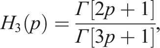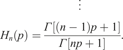²² Fokker and Planck devised the Fokker-Planck (FP) equation to theoretically understand a Brownian movement and fluctuations of probability distributions for stochastic processes in both temporal and spatial ranges. A second-order unbounded expansion can then derive the FP equation (FPE) from the Kramers–Moyal expansion of the master equation. The chemical master equation is the angular noise approximation version, which allows for obtaining a more exact version. FPE, the main feature of the so-called mathematical technique, is widely applicable to many natural science processes. However, these are among many other models like the probability flux, polymer dynamics, electron relaxation, solid state systems, and quantum optics. The primary aim of our work is to investigate FFPE, which the following generic form can describe

$D_t^{\rho }\eta ={\partial }_x\eta +{\partial }_x^2\eta ,$

(1)with the initial condition (IC)

$\eta \left(x,t_0\right)=g\left(x\right),$

(2)where $\eta \equiv \eta \left(x,t\right)$ and the fractional order parameter $0<\rho \le 1$ .

The FFP equation (FFPE) has proved efficient in many fields, such as biological molecules, chemical physics, energy consumption, and optical fiber.^23,24 The existing FFPE has been extended to deal with internal properties, mechanical behavior, and diffusion phenomena. ¹⁷ For instance, it is usually quite challenging to secure accurate data that can be used to solve the FDEs. Therefore, various analytical and numerical techniques indulge these curious minds. Examples of advanced numerical methods are the Laplace transform method (LTM), ¹⁸ the multistep reduced differential transform method (MRDTM), ²⁵ the predictor-corrector approach, ²⁶ the Adomian decomposition method (ADM), ²⁷ and the variational iteration method (VIM). ²⁸ They are used to tackle diffusion-type odes. Marinca et al. ²⁹ formulated an optimal auxiliary function to derive the analytical solutions for the flow of fourth-grade fluids from an endless vertical cylinder.

Meanwhile, in 2013, Laiq Zada and his coauthors ³⁰ published another article regarding a new method to solve PDEs, especially the seventh-order generalized Korteweg-de Vries (KdV) equation. As you have read, the finding resulted from modifying the technique. The proposed approach considers additional convergence control parameters and functions to ensure the method converges quickly and smoothly. The strategy efficiency can be altered either by modifying the accessory service or by increasing the number of convergence control auxiliary tuning knobs.

The primary objective of this study is to develop a novel technique, referred to for the first time as the “ Tantaway Technique ,” to address the FFP problems in a straightforward and uncomplicated manner. This technique is distinguished by its high accuracy across the study domain and superior speed compared to alternative methods. Moreover, the findings produced by the “Tantaway Technique” will be compared with the approximations derived by the OAFM and the Laplace homotopy perturbation method (LHPM).

Preliminaries

This section provides an overview of fundamental terminology and conclusions about the Caputo fractional derivative.

Definition 2.1: The expression denoting the Riemann fractional integral of the function $\eta \left(x,t\right)$ can be represented by 31

$I_t^{\rho }\left[\eta \left(x,t\right)\right]=\frac{1}{\Gamma \left[\rho \right]}{{\int }_0^t\left(t-r\right)}^{\rho -1}\eta \left(x,r\right)dr,$

(3)and $I_t^0\left[\eta \left(x,t\right)\right]=\eta \left(x,t\right).$

Definition 2.2: The fractional derivative of the function $\eta \equiv \eta \left(x,t\right)$ , according to the Caputo derivative formula, is given by ³¹

$D_t^{\rho }\eta \left(x,t\right)=\frac{1}{\Gamma \left[m-\rho \right]}{{\int }_0^t\left(t-r\right)}^{m-\rho -1}{\partial }_r^m\eta \left(x,r\right),m-1<\rho \le m\hspace{0.17em}\&\hspace{0.17em}t>0.$

(4)

Lemma 1

For $n-1<\rho \le n,t\ge 0$ and $\lambda \in R$ , we have

• $D_t^{\rho }{t}^k=\frac{\Gamma \left(k+1\right)}{\Gamma \left(k+1-\rho \right)}{t}^{k-\rho }$

• $D_t^{\rho }{I}_t^{\rho }\eta \left(x,t\right)=\eta \left(x,t\right),$

• $I_t^{\rho }{t}^k=\frac{\Gamma \left(k+1\right)}{\Gamma \left(k+\rho +1\right)}{t}^{k+\rho }$

• $I_t^{\rho }{D}_t^{\rho }\left(\eta \left(x,t\right)\right)=\eta \left(x,t\right)-{\displaystyle \sum }_{i=0}^{n-1}{\partial }^i\eta \left(x,0\right)\frac{t^i}{i!}.$

General procedure for the OAFM

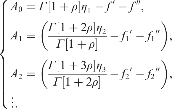
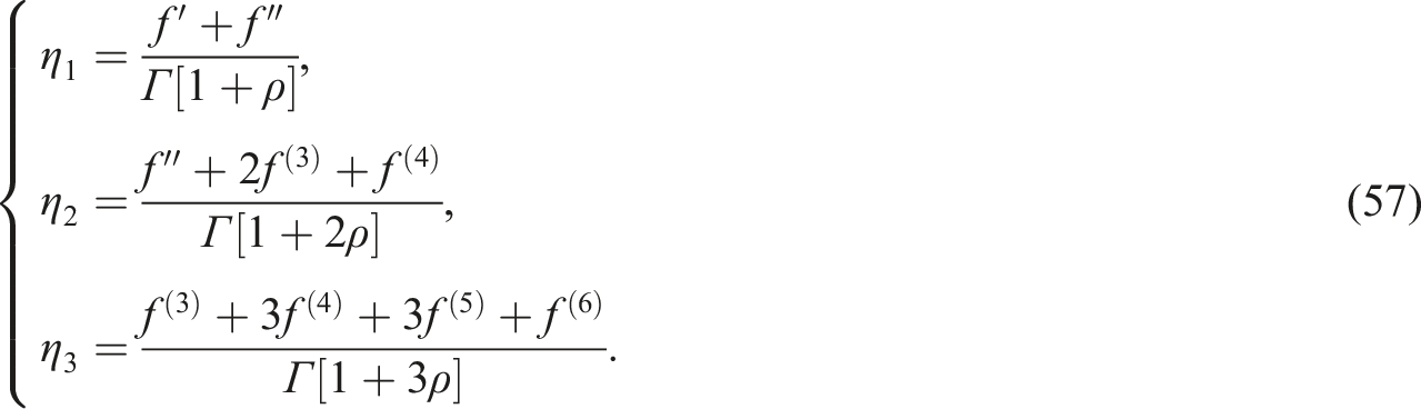
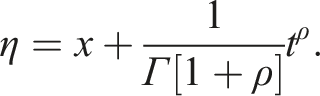
Here, we present a concise and straightforward explanation of the OAFM, which can be used to analyze fractional PDEs. ³² First, the following FPDE is introduced to apply the suggested method

$D_t^{\rho }\eta \left(x,t\right)=L\left[\eta \left(x,t\right)\right]=g\left(x,t\right)+N\left[\eta \left(x,t\right)\right],$

(5)which is subjected to the IC

$D_t^k\eta =h_k\left(x\right),$

(6)where $D_t^{\rho }\equiv {\partial }^{\rho }/t^{\rho }$ represents the Caputo operator, $\eta \equiv \eta \left(x,t\right)$ is an unknown function, and $g\equiv g\left(x,t\right)$ indicates a known analytic function. The following concise steps are outlined to implement the recommended approach:

• Step (1): To solve equation (5) and produce an approximate solution that has two components, we introduce the following formula

$\eta \left(x,t\right)={\eta }_0\left(x,t\right)+{\eta }_1\left(x,t,C_i\right),i=1,2,3,\dots ,p$

(7)

• Step (2): To get the zeroth- and first-order approximations, we insert equation (7) into equation (5), which leads to the following outcome:

$L\left[{\eta }_0\left(x,t\right)\right]+L\left[{\eta }_1\left(x,t\right)\right]-g\left(x,t\right)-N\left[{\eta }_0\left(x,t\right)+{\eta }_1\left(x,t,C_i\right)\right]=0.$

(8)

• Step (3): To derive the zeroth-order approximation ${\eta }_0\left(x,t\right)$ , for the linear equation, we use

$\frac{{\partial }^{\rho }{\eta }_0\left(x,t\right)}{\partial t^{\rho }}-g\left(x,t\right)=0,$

(9)and by applying the inverse operator on equation (9) with using the IC equation (6), we obtain

${\eta }_0\left(x,t\right)=g\left(x,t\right).$

(10)

• Step (4): From equation (8), the term $N\left[{\eta }_0\left(x,t\right)+{\eta }_1\left(x,t,C_i\right)\right]$ can be expressed by

$N\left[{\eta }_0\left(x,t\right)+{\eta }_1\left(x,t,C_i\right)\right]=N\left[{\eta }_0\left(x,t\right)\right]+{\displaystyle \sum }_{k=1}^{\infty }\frac{{\eta }_1^k}{k!}{N}^{\left(k\right)}\left[{\eta }_0\left(x,t\right)\right].$

(11)

• Step (5): To expedite the solution of equation (11) and enhance the rate of convergence for the first-order approximation ${\eta }_1\left(x,t\right)$ , we propose an alternate formulation expressed as

$L\left[{\eta }_1\left(x,t\right)\right]+T_1\left[\left({\eta }_0\left(x,t\right),C_i\right)\right]N\left[{\eta }_0\left(x,t\right)\right]+T_2\left[\left({\eta }_0\left(x,t\right),C_j\right)\right]=0,$

(12)with $D_t^k{\eta }_1\left(x,t\right)=0,$ and $\left(T_1,T_2\right)$ are appropriate auxiliary functions (AFs).

• Step (6): The first-order approximation ${\eta }_1\left(x,t\right)$ , is derived by applying the inverse operator to equation (12) after inserting the AFs.

• Step (7): Determining the convergence control parameters $C_i$ involves various procedures, including least squares, Galerkin’s method, Riz method, and collocation. The least squares technique is employed to increase the accuracy of the approximations and minimize their errors

$J\left(C_i,C_j\right)={\int }_0^t{\int }_{\Omega }{R}^2\left(x,t,C_i,C_j\right)dxdt$

(13)where $R$ denotes the residual,

$R\left(x,t,C_i,C_j\right)=\frac{\partial {\eta }^{\rho }\left(x,t,C_i,C_j\right)}{\partial t^{\rho }}-g\left(x,t\right)-N\left[\eta \left(x,t,C_i,C_j\right)\right],$

(14)where $i=1,2,\dots ,s\hspace{0.17em}\&\hspace{0.17em}j=s+1,s+2,\dots ,p.$

General procedure for the “Tantawy technique”

Due to the innovative nature of this technique and its initial mention here, stemming from the publication delay of Prof. El-Tantawy and Prof. Alvaro Salas’s paper, it is imperative to acknowledge that Prof. El-Tantawy and Prof. Salas are responsible for its intricacies. Consequently, all credit for this technique is attributed to him, and it has been named in his honor to safeguard the rights of all parties involved.

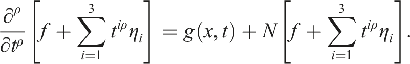
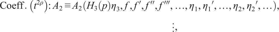
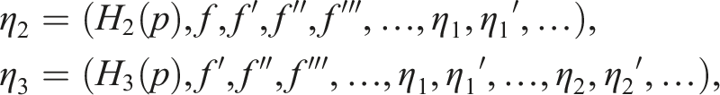
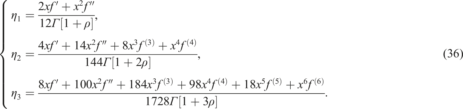
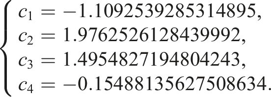
The subsequent points will elucidate the Tantawy technique for analyzing fractional differential equations and several intricate physical and engineering problems:

Step (1): To solve the IVP (5), the following Ansatz is introduced

$\eta \left(x,t\right)=f\left(x\right)+{\displaystyle \sum }_{i=1}^{\infty }{t}^{i\rho }{\eta }_i\left(x\right),i=1,2,3,\cdots ,=f+{\displaystyle \sum }_{i=1}^{\infty }{t}^{i\rho }{\eta }_i,$

(15)where ${\eta }_0\left(x\right)=f\left(x\right)\equiv f$ indicates the IC and ${\eta }_i\equiv {\eta }_i\left(x\right)$ are undetermined functions only in the variable $x$ .

• Step (2): Insert the Ansatz (15) into equation (5) yields

$\frac{{\partial }^{\rho }}{\partial t^{\rho }}\left[f+{\displaystyle \sum }_{i=1}^{\infty }{t}^{i\rho }{\eta }_i\right]=g\left(x,t\right)+N\left[f+{\displaystyle \sum }_{i=1}^{\infty }{t}^{i\rho }{\eta }_i\right],$

(16)which for N ^th -terms in the series solution (say N = 3), we get

$\frac{{\partial }^{\rho }}{\partial t^{\rho }}\left[f+{\displaystyle \sum }_{i=1}^3{t}^{i\rho }{\eta }_i\right]=g\left(x,t\right)+N\left[f+{\displaystyle \sum }_{i=1}^3{t}^{i\rho }{\eta }_i\right].$

• Step (3): Collecting the coefficients of the same power of $t^{i\rho }$ after using the definition of the Caputo fractional derivative operator (CFDO), we get

$A_0+A_1{t}^{\rho }+A_2{t}^{2\rho }+A_3{t}^{3\rho }+\cdots =0,$

with the following coefficients

$\text{Coeff}.\hspace{0.17em}\left(t^{0\rho }\right):A_0\equiv A_0\left(H_1\left(p\right){\eta }_1,f,f^{\prime },f^{″},f^{‴},\dots \right),$

$\text{Coeff}.\hspace{0.5em}\left(t^{\rho }\right):A_1\equiv A_1\left(H_2\left(p\right){\eta }_2,f,f^{\prime },f^{″},f^{‴},\dots ,{\eta }_1,{{\eta }_1}^{\prime },\dots \right),$

$\text{Coeff}.\hspace{0.17em}\left(t^{2\rho }\right):A_2\equiv A_2\left(H_3\left(p\right){\eta }_3,f,f^{\prime },f^{″},f^{‴},\dots ,{\eta }_1,{{\eta }_1}^{\prime },\dots ,{\eta }_2,{{\eta }_2}^{\prime },\dots \right),\begin{array}{llllllllll}& & & & & & & & & ⋮,\end{array}$

with

$H_1\left(p\right)=\frac{1}{\Gamma \left[p+1\right]},$

$H_2\left(p\right)=\frac{\Gamma \left[p+1\right]}{\Gamma \left[2p+1\right]},$

$H_3\left(p\right)=\frac{\Gamma \left[2p+1\right]}{\Gamma \left[3p+1\right]},$

$\begin{array}{llll}& & & ⋮\end{array}{H}_n\left(p\right)=\frac{\Gamma \left[\left(n-1\right)p+1\right]}{\Gamma \left[np+1\right]}.$

• Step (4): Equating to zero the coefficients $A_i$ for $i=0,1,2,\cdots ,$ and solving the obtained system in ${\eta }_i\equiv {\eta }_i\left(x\right)$ for $i=1,2,3,\cdots$ , we can get

${\eta }_1=\left(H_1\left(p\right),f,f^{\prime },f^{″},f^{‴},\dots \right),$

${\eta }_2=\left(H_2\left(p\right),f,f^{\prime },f^{″},f^{‴},\dots ,{\eta }_1,{{\eta }_1}^{\prime },\dots \right),{\eta }_3=\left(H_3\left(p\right),f^{\prime },f^{″},f^{‴},\dots ,{\eta }_1,{{\eta }_1}^{\prime },\dots ,{\eta }_2,{{\eta }_2}^{\prime },\dots \right),$

• Step (5): By inserting the obtained values of ${\eta }_i\equiv {\eta }_i\left(x\right)$ into the Ansatz (15), we can obtain an approximate solution for the suggested problem.

Test examples and numerical investigation

Let us apply the proposed method’s previous steps to analyze and model some fractional differential equations with multiple applications in different physical systems. Below, we will discuss some other forms of the Fractional Fokker–Plank equation (FFPE).

Example (1)

Consider the following first model of the FFPE

${D_t}^{\rho }\eta -{\partial }_x\left(\frac{x}{6}\eta \right)-{\partial }_x^2\left(\frac{x^2}{12}\eta \right)=0,$

(17)which is subjected to the following IC

$\eta \left(x,0\right)\equiv {\eta }_0=f=x^2.$

(18)Here, $\eta \equiv \eta \left(x,t\right)$ , and $0<\rho \le 1.$

The OAFM for analyzing example (1)

Consider the following terms of equation (17),

$L\left(\eta \right)=D_t^{\rho }\eta ,$

(19)

$N\left(\eta \right)={\partial }_x\left(\frac{x}{6}\eta \right)-{\partial }_{x,x}\left(\frac{x^2}{12}\eta \right),$

(20)and

$g\left(x,t\right)=0.$

(21)

The initial approximation/IC, according to OAFM, reads

$D_t^{\rho }{\eta }_0\left(x,t\right)=0,$

(22)

Applying the inverse operator on equation (22) yields

$\eta \left(x,0\right)\equiv {\eta }_0=x^2.$

(23)

Using equation (23) in equation (20), the following term is obtained

$N\left[{\eta }_0\left(x,t\right)\right]=-\frac{x^2}{2} .$

(24)

According to the OAFM procedure, the first approximation reads

$D_t^{\rho }{\eta }_1=-T_1\left[{\eta }_0,C_i\right]N\left[{\eta }_0\right]-T_2\left[{\eta }_0,C_j\right].$

(25)

We choose the following auxiliary function

$T_1=c_1{\left(x^2\right)}^3+c_2{\left(x^2\right)}^4,$

(26)

$T_2=c_3{\left(x^2\right)}^7 .$

(27)

After substituting equations (24), (26), and (27) into equation (25), we get

$D_t^{\rho }{\eta }_1=-c_1{x}^6-c_2{x}^8+\frac{1}{2}{c}_3{x}^{16}.$

(28)

Applying the inverse operator on equation (28) yields

${\eta }_1=\frac{t^{\rho }{x}^6\left(-2c_1-2c_{2}2x^2+c_3{x}^{10}\right)}{2\rho \Gamma \left[\rho \right]}.$

(29)

Collecting equations (23) and (29), we get

$\eta \left(x,t\right)={\eta }_0+{\eta }_1=x^2+\frac{t^{\rho }{x}^6\left(-2c_1-2c_{2}2x^2+c_3{x}^{10}\right)}{2\rho \Gamma \left[\rho \right]}.$

(30)

Applying the least square technique, the following values of auxiliary constants are obtained

$\{\begin{array}{l}{c}_1=-2.073345190444604,\\ c_2=1.9430049027565428,\\ c_3=0.40613292934774126.\end{array}$

(31)

The final solution using auxiliary constant reads

$\eta \left(x,t\right)=x^2+x^6\left(0.406133x^{10}-3.88601x^2+4.14669\right)\frac{t^{\rho }}{2\rho \Gamma \left[\rho \right]}.$

(32)

The Tantawy technique for analyzing example (1)

Here, the Tantawy technique is introduced to analyze example (1). This technique is summarized in the following brief steps:

Step (1): To solve the IVP (17), the following Ansatz is introduced

$\eta =f+t^{\rho }{\eta }_1+t^{2\rho }{\eta }_2+t^{3\rho }{\eta }_3+\cdots ,$

(33)where ${\eta }_0\equiv f=x^2$ indicates the initial solution/condition and ${\eta }_i\equiv {\eta }_i\left(x\right)$ for $i=1,2,3,\cdots ,$ are undetermined functions in the variable $x$ only.

• Step (2): Inserting the Ansatz (33) into equation (17) to find the values of the unknown functions ${\eta }_i\equiv {\eta }_i\left(x\right)$ , which leads to the following outcome:

$\frac{{\partial }^{\rho }}{\partial t^{\rho }}\left[f+t^{\rho }{\eta }_1+t^{2\rho }{\eta }_2+t^{3\rho }{\eta }_3+\cdots \right]={\partial }_x\left[\frac{x}{6}\left(f+t^{\rho }{\eta }_1+t^{2\rho }{\eta }_2+t^{3\rho }{\eta }_3+\cdots \right)\right]+{\partial }_x^2\left[\frac{x^2}{12}\left(f+t^{\rho }{\eta }_1+t^{2\rho }{\eta }_2+t^{3\rho }{\eta }_3+\cdots \right)\right].$

(34)

• Step (3): Collecting the coefficients of the same power of $t^{i\rho }$ and after using the definition of the CFDO, we get

$A_0+A_1{t}^{\rho }+A_2{t}^{2\rho }+\cdots =0,$

(35)with

$\{\begin{array}{l}{A}_0=\Gamma \left[1+\rho \right]{\eta }_1-\frac{1}{6}x{f}^{\prime }-\frac{1}{12}{x}^2{f}^{″},\\ A_1=\left(\frac{\Gamma \left[1+2\rho \right]}{\Gamma \left[1+\rho \right]}{\eta }_2-\frac{1}{6}x{f_1}^{\prime }-\frac{1}{12}{x}^2{f_1}^{″}\right),\\ A_2=\left(\frac{\Gamma \left[1+3\rho \right]}{\Gamma \left[1+2\rho \right]}{\eta }_3-\frac{1}{6}x{f_2}^{\prime }-\frac{1}{12}{x}^2{f_2}^{″}\right),\\ ⋮.\end{array}$

• Step (4): Equating to zero the coefficients $A_i$ for $i=0,1,2,$ and solving the obtained system ${\eta }_i\equiv {\eta }_i\left(x\right)$ , we finally get the explicit values of ${\eta }_i\equiv {\eta }_i\left(x\right)$ as follows

$\{\begin{array}{l}{\eta }_1=\frac{2x{f}^{\prime }+x^2{f}^{″}}{12\Gamma \left[1+\rho \right]},\\ {\eta }_2=\frac{4x{f}^{\prime }+14x^2{f}^{″}+8x^3{f}^{\left(3\right)}+x^4{f}^{\left(4\right)}}{144\Gamma \left[1+2\rho \right]},\\ {\eta }_3=\frac{8x{f}^{\prime }+100x^2{f}^{″}+184x^3{f}^{\left(3\right)}+98x^4{f}^{\left(4\right)}+18x^5{f}^{\left(5\right)}+x^6{f}^{\left(6\right)}}{1728\Gamma \left[1+3\rho \right]}.\end{array}$

(36)

• Step (5): Inserting the value of IC $f=x^2$ into equation (36), the explicit values ${\eta }_i\equiv {\eta }_i\left(x\right)$ are obtained

${\eta }_1=\frac{x^2}{2\Gamma \left[1+\rho \right]},{\eta }_2=\frac{x^2}{4\Gamma \left[1+2\rho \right]},{\eta }_3=\frac{x^2}{8\Gamma \left[1+3\rho \right]}.$

(37)

• Step (6): Inserting the obtained values of ${\eta }_i\equiv {\eta }_i\left(x\right)$ into the Ansatz (33), an approximate solution for the suggested problem is finally obtained

$\eta =x^2+\frac{x^2}{2\Gamma \left[1+\rho \right]}{t}^{\rho }+\frac{x^2}{4\Gamma \left[1+2\rho \right]}{t}^{2\rho }+\frac{x^2}{8\Gamma \left[1+3\rho \right]}{t}^{3\rho }+\cdots .$

(38)

The residual error for this approximation reads

$R=-\frac{x^2}{16\Gamma \left[1+3\rho \right]}{t}^{3\rho }.$

Utilizing Laplace HPM (LHPM) and following extensive computations and significant time expenditure, we obtain findings identical to those produced by the Tantawy technique

$\eta =x^2+\frac{x^2}{2\Gamma \left[1+\rho \right]}{t}^{\rho }+\frac{x^2}{4\Gamma \left[1+2\rho \right]}{t}^{2\rho }+\frac{x^2}{8\Gamma \left[1+3\rho \right]}{t}^{3\rho }+\cdots .$

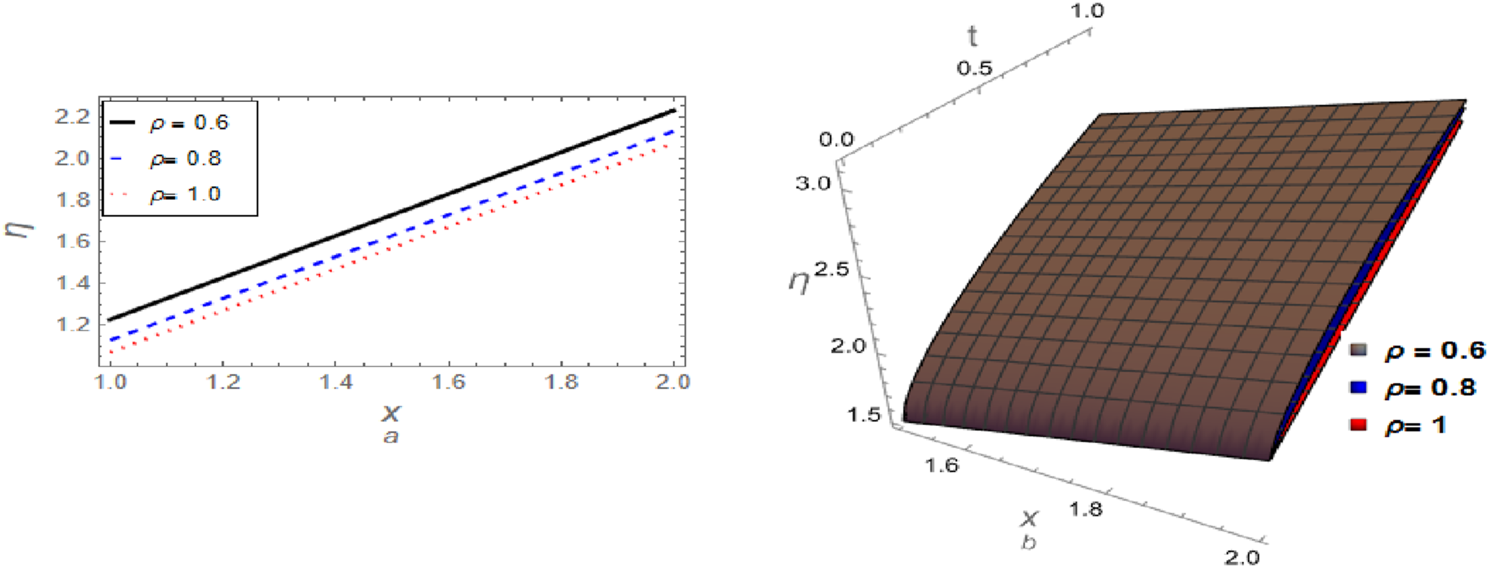
The approximations (32) and (38) using OAFM and the Tantawy technique are, respectively, depicted in Figures 1 and 2 for various values to the fractional order parameter $\rho$ . These figures show how strong the effect of ρ is on the behavior of the derived approximations. Moreover, in Figure 3, we juxtaposed the approximations (32) and (38) with the exact solution of the integer case to measure the concordance between the generated approximations and the exact solution for the integer case. Figure 3 demonstrates that the derived approximations align closely with the exact solution of the integer case in the short domain; however, in the long domain, the approximation (32) obtained through OAFM diverges from the exact solution, whereas the approximation (38) derived from Tantawy’s technique exhibits complete concordance, thereby enhancing the accuracy and efficiency of Tantawy’s approach. This consequently suggests favorable outcomes in analyzing diverse physical and engineering problems. We also estimated the absolute error $R_{\infty }=\left|\text{Exact}‐\text{Approx}.\right|$ for the approximations (32) and (38), as shown in Figures 4 and 5, respectively. This figure unequivocally demonstrates that Tantawy’s technique is superior to OAFM over the whole study domain.

Figure 1.

The behavior of fractional approximation (32) using OAFM at various values of fractional order parameter for example 1 (a) two-dimensional graph at $t=0.07$ and (b) three-dimensional graph.

Figure 2.

The behavior of fractional approximation (38) using Tantawy technique at various values of fractional order parameter for example 1 (a) two-dimensional graph at $t=0.07$ and (b) three-dimensional graph.

Figure 3.

A comparison between the derived approximations (32) and (38) with the exact solution (3) for the integer case at $t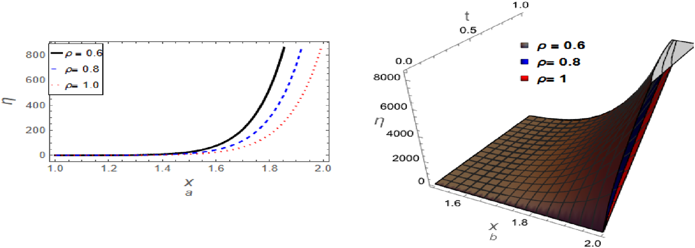=0.07$ (a) for the short domain (small $x$ ) and (b) for the long domain (large $x$ ).

Figure 4.

The absolute error $R_{\infty }$ for the derived approximations (32) at $\rho =1$ : (a) three-dimensional graph and (b) two-dimensional graph at $t=0.001$ .

Figure 5.

The absolute error $R_{\infty }$ for the derived approximations (38) at $\rho =1$ : (a) three-dimensional graph and (b) two-dimensional graph at $t=0.001$ .

Example (2)

Considering the following second model of FFPE

${D_t}^{\rho }\eta -{\partial }_x\eta -{\partial }_x^2\eta =0,$

(39)which is subjected to the IC

$\eta \left(x,0\right)\equiv {\eta }_0\equiv f=x,$

(40)where $\eta \equiv \eta \left(x,t\right)$ and $0<\rho \le 1.$

We apply the two proposed techniques for analyzing this model as follows.

The OAFM for analyzing example (2)

The following terms of equation (39) are introduced

$L\left[\eta \right]=D_t^{\rho }\eta ,$

(41)

$N\left[\eta \right]=-{\partial }_x\eta -{\partial }_x^2\eta ,$

(42)and

$g\left(x,t\right)=0.$

(43)

The initial approximation/IC, according to the OAFM, reads

$D_t^{\rho }{\eta }_0\left(x,t\right)=0.$

(44)

Applying the inverse operator on equation (44) yields

${\eta }_0=x.$

(45)

Using equation (45) in equation (41), we get

$N\left[{\eta }_0\right]=-1.$

(46)

According to the OAFM procedure, the first approximation reads

$D_t^{\rho }{\eta }_1=-T_1\left[{\eta }_0,C_i\right]N\left[{\eta }_0\right]-T_2\left[{\eta }_0,C_j\right].$

(47)

The following auxiliary function is introduced

$T_1=c_1{\left(x\right)}^3+c_2{\left(x\right)}^5,$

(48)

$T_2=c_3{\left(x\right)}^6+c_4{\left(x\right)}^9.$

(49)

After substituting equations (45), (48), and (49) into equation (47), we get

$D_t^{\rho }{\eta }_1=c_1{x}^3+c_2{x}^5-c_3{x}^6-c_4{x}^9.$

(50)

Applying the inverse operator on equation (50) yields

${\eta }_1=\frac{t^{\rho }{x}^3\left(c_1+c_2{x}^2-c_3{x}^3-c_4{x}^6\right)}{\rho \Gamma \left[\rho \right]}.$

(51)

Now, by collecting equations (45) and (51), the following OAFM solution is obtained

$\eta \left(x,t\right)={\eta }_0+{\eta }_1=x+\frac{t^{\rho }{x}^3\left(c_1+c_2{x}^2-c_3{x}^3-c_4{x}^6\right)}{\rho \Gamma \left[\rho \right]},$

(52)with the following values of the auxiliary constants

$\{\begin{array}{l}{c}_1=-1.1092539285314895,\\ c_2=1.9762526128439992,\\ c_3=1.4954827194804243,\\ c_4=-0.15488135627508634.\end{array}$

Now, by inserting the obtained values if auxiliary constants in equation (53), the following approximation is obtained

$\eta \left(x,t\right)=x+\left(0.154881x^9-1.49548x^6+1.97625x^5-1.10925x^3\right)\frac{t^{\rho }}{\rho \Gamma \left[\rho \right]}.$

(53)

The Tantawy technique for analyzing example (2)

The Tantawy technique can be utilized to examine example (2) by delineating the subsequent points:

Step (1): To solve and analyze the IVP (39), the following Ansatz is introduced

$\eta =f+t^{\rho }{\eta }_1+t^{2\rho }{\eta }_2+t^{3\rho }{\eta }_3+\cdots ,$

(54)where ${\eta }_0\equiv f=x$ indicates the initial solution/condition and ${\eta }_i\equiv {\eta }_i\left(x\right)$ for $i=1,2,3,\cdots ,$ are undetermined functions.

• Step (2): To determine the values of the unknown functions ${\eta }_i\equiv {\eta }_i\left(x\right)$ , we insert the Ansatz (54) into equation (39), which leads to the following equation:

$\frac{{\partial }^{\rho }}{\partial t^{\rho }}\left[f+t^{\rho }{\eta }_1+t^{2\rho }{\eta }_2+t^{3\rho }{\eta }_3+\cdots \right]={\partial }_x\left[\left(f+t^{\rho }{\eta }_1+t^{2\rho }{\eta }_2+t^{3\rho }{\eta }_3+\cdots \right)\right]+{\partial }_x^2\left[\left(f+t^{\rho }{\eta }_1+t^{2\rho }{\eta }_2+t^{3\rho }{\eta }_3+\cdots \right)\right].$

(55)

• Step (3): Collecting the coefficients of the same power of $t^{i\rho }$ and after using the definition of the CFDO, we get

$A_0+A_1{t}^{\rho }+A_2{t}^{2\rho }+\cdots =0,$

(56)with

$\{\begin{array}{l}{A}_0=\Gamma \left[1+\rho \right]{\eta }_1-f^{\prime }-f^{″},\\ A_1=\left(\frac{\Gamma \left[1+2\rho \right]{\eta }_2}{\Gamma \left[1+\rho \right]}-{f_1}^{\prime }-{f_1}^{″}\right),\\ A_2=\left(\frac{\Gamma \left[1+3\rho \right]{\eta }_3}{\Gamma \left[1+2\rho \right]}-{f_2}^{\prime }-{f_2}^{″}\right),\\ ⋮.\end{array}$

• Step (4): Equating to zero the coefficients $A_i$ for $i=0,1,2,$ and solving them in ${ƞ}_j$ , we finally get the explicit values of ${\eta }_i\equiv {\eta }_i\left(x\right)$ as follows

$\{\begin{array}{l}{\eta }_1=\frac{f^{\prime }+f^{″}}{\Gamma \left[1+\rho \right]},\\ {\eta }_2=\frac{f^{″}+2f^{\left(3\right)}+f^{\left(4\right)}}{\Gamma \left[1+2\rho \right]},\\ {\eta }_3=\frac{f^{\left(3\right)}+3f^{\left(4\right)}+3f^{\left(5\right)}+f^{\left(6\right)}}{\Gamma \left[1+3\rho \right]}.\end{array}$

(57)

• Step (5): Inserting the value of IC $f=x$ into equation (57), the values of ${\eta }_i\equiv {\eta }_i\left(x\right)$ are obtained as follows

${\eta }_1=\frac{1}{\Gamma \left[1+\rho \right]},{\eta }_2=0,{\eta }_3=0.$

(58)

• Step (6): Inserting the obtained values of ${\eta }_i\equiv {\eta }_i\left(x\right)$ into the Ansatz (54), we finally get the exact solution for the suggested problem as follows

$\eta =x+\frac{1}{\Gamma \left[1+\rho \right]}{t}^{\rho }.$

(59)

The residual error for this approximation equals to zero.

Utilizing Laplace HPM (LHPM) and following extensive computations and significant time expenditure, we obtain findings identical to those produced by the Tantawy technique

$\eta =x+\frac{1}{\Gamma \left[1+\rho \right]}{t}^{\rho }.$

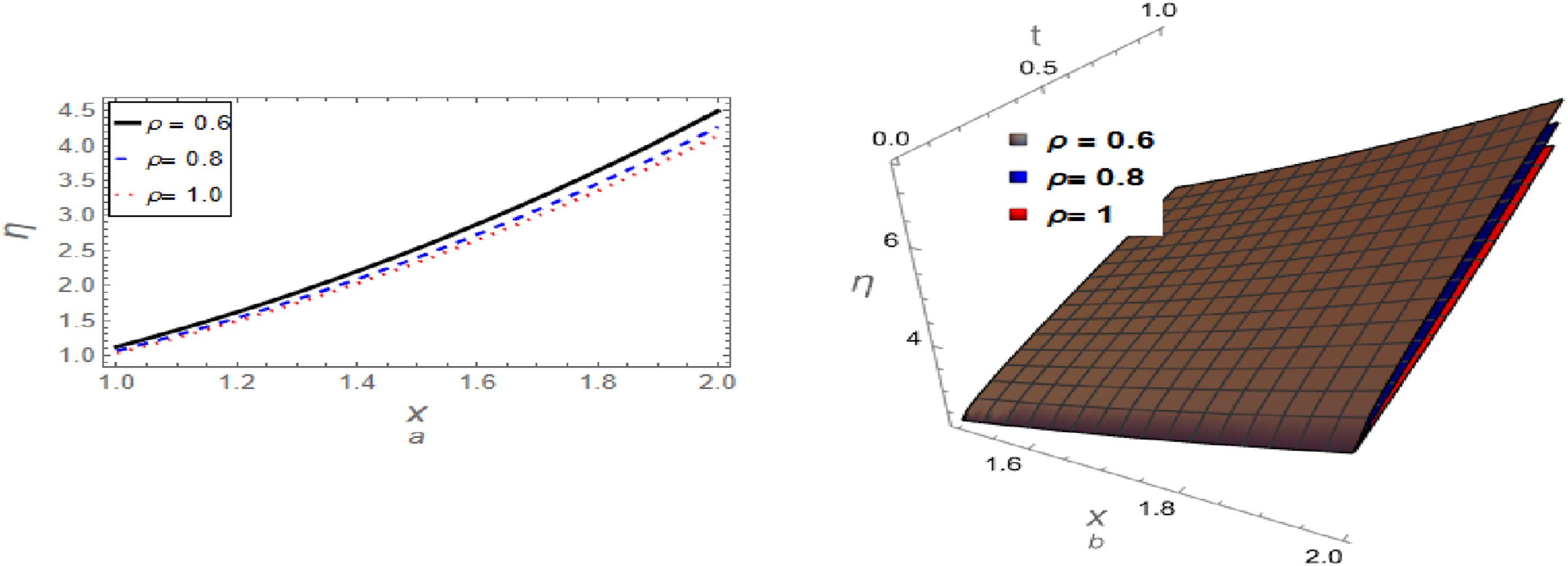
Figures 6 and 7 illustrate the graphic analysis of the approximation (53) using OAFM and the approximation (59) using the Tantawy technique for various values of the fractional order parameter ρ. These figures clearly show that the fractional coefficient dramatically influences the behavior of the phenomena described by this model. Therefore, this effect can expose the ambiguity surrounding certain behaviors observed in the phenomena that this model studied.

Figure 6.

The behavior of fractional approximation (53) using OAFM at various values of fractional order parameter for example (2): (a) two-dimensional graph at $t=0.07$ and (b) three-dimensional graph.

Figure 7.

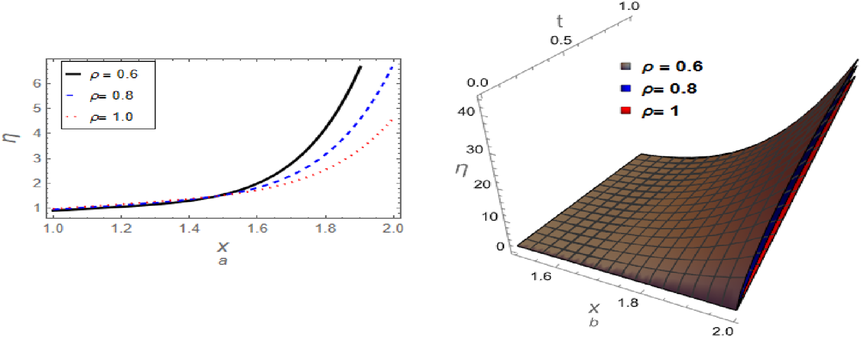
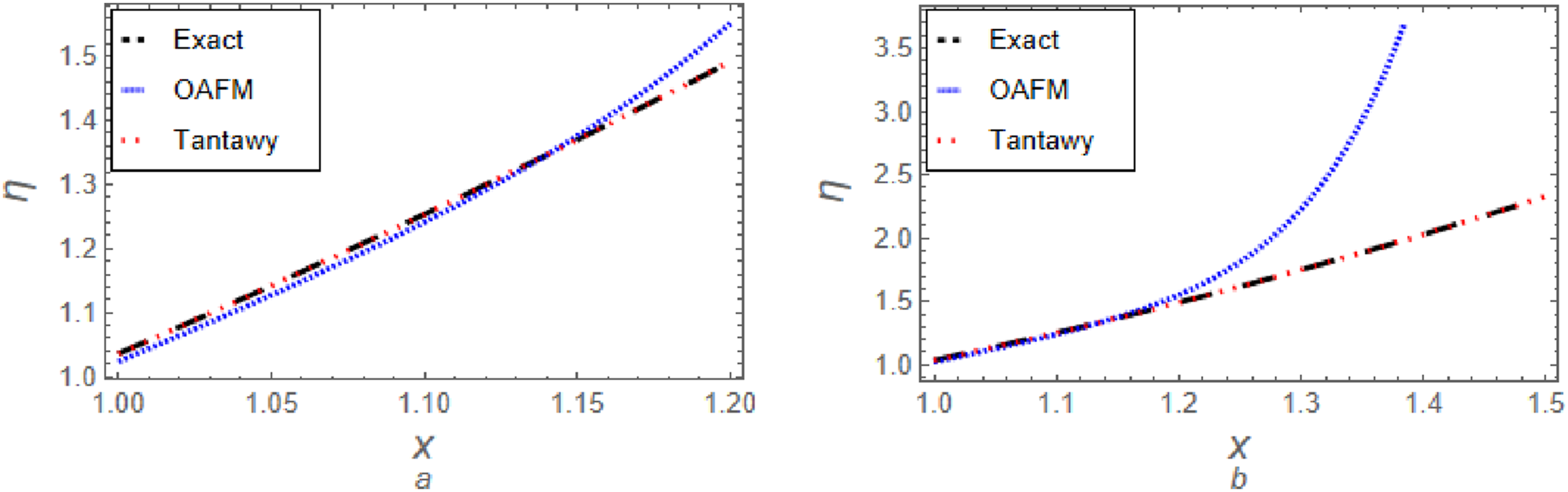
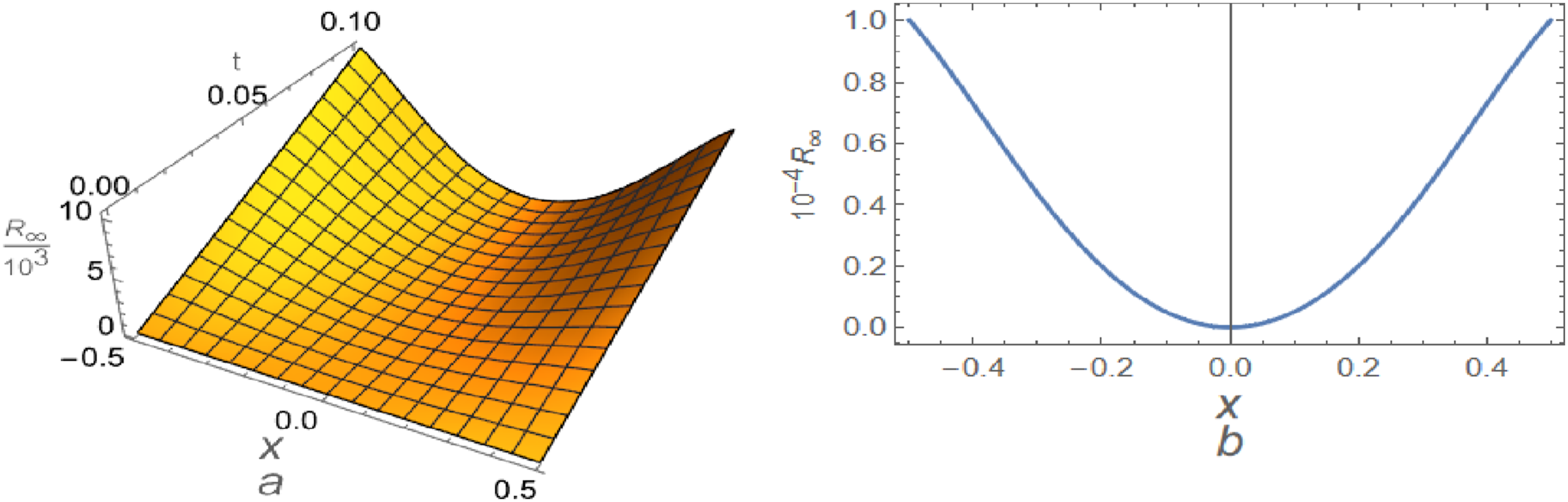
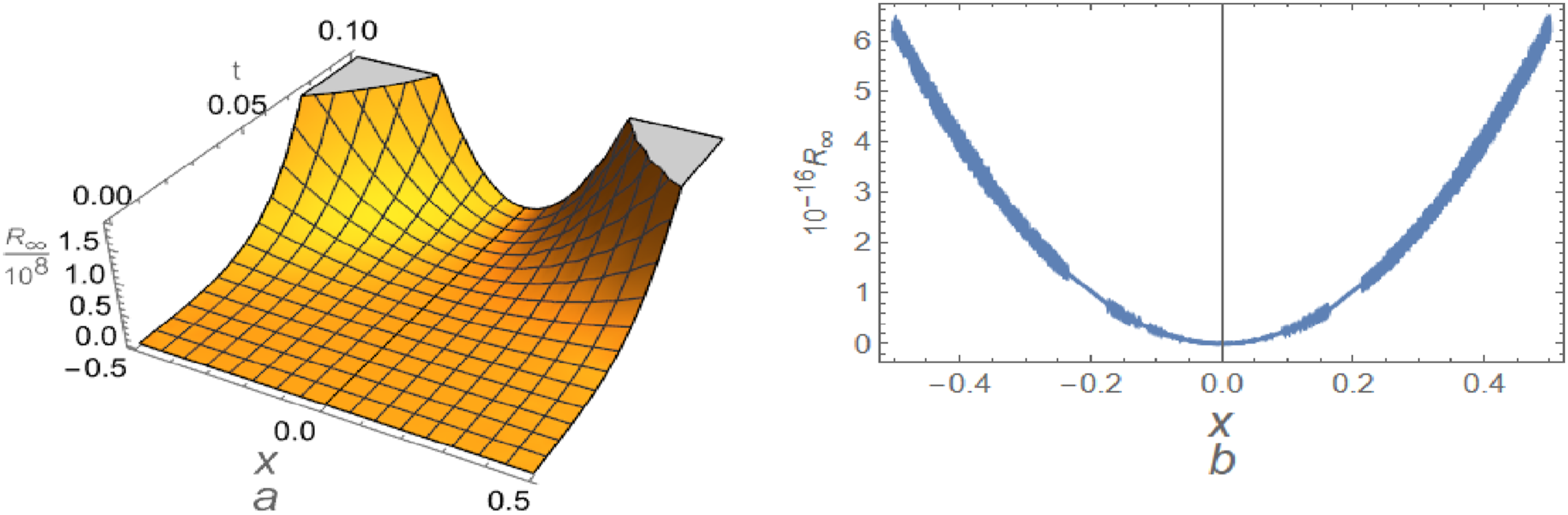
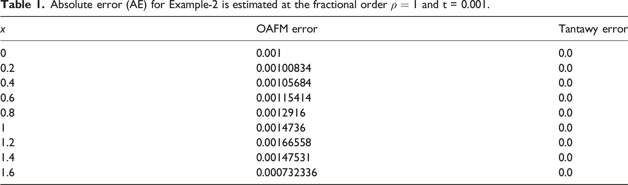
The behavior of fractional approximation (59) using Tantawy technique at various values of fractional order parameter for example (2): (a) two-dimensional graph at $t=0.07$ and (b) three-dimensional graph.

Additionally, in Figure 8, we compared the exact solution of the integer case (ρ = 1) with the approximations (53) and (59) to assess the concordance between the generated approximations and the exact solution. It is found that, in a short time, the derived approximations closely align with the exact solution of the integer case, as illustrated in Figure 8(a). However, over a long time, the approximation (53) obtained through OAFM diverges from the exact solution, whereas the approximation (59) derived from Tantawy’s technique achieves complete concordance, as shown in Figure 8(b)), which conforms to the high accuracy for the obtained solution via Tantawy’s approach. Consequently, this implies that analyzing a wide range of physical and engineering problems will yield favorable results using Tantawy’s approach. Moreover, we numerically calculated the absolute error of both approximations, as illustrated in Table 1. The efficiency and accuracy of Tantawy’s technique are demonstrated in this table compared to OAFM.

Figure 8.

A comparison between the derived approximations (53) and (59) with the exact solution $\eta =x+t$ for the integer case (a) at a short time $t=0.001$ and (b) at a long time $t=0.1$ .

Table 1.

Absolute error (AE) for Example-2 is estimated at the fractional order 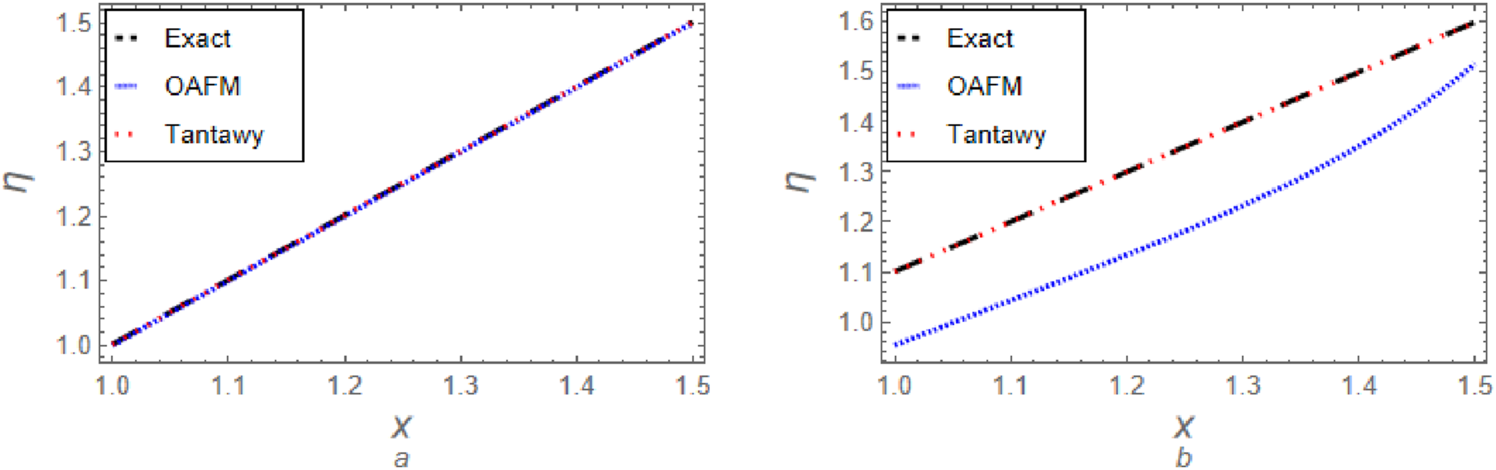$\rho =1$ and t = 0.001.

$x$	OAFM error	Tantawy error
0	0.001	0.0
0.2	0.00100834	0.0
0.4	0.00105684	0.0
0.6	0.00115414	0.0
0.8	0.0012916	0.0
1	0.0014736	0.0
1.2	0.00166558	0.0
1.4	0.00147531	0.0
1.6	0.000732336	0.0

Example (3)

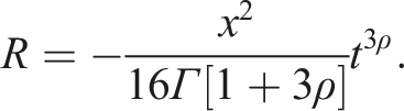
Considering the following third form of the FFPE

$D_t^{\rho }\eta +{\partial }_x\left(\frac{4}{x}{\eta }^2\right)-{\partial }_x\left(\frac{x}{3}\eta \right)-{\partial }_x^2{\eta }^2=0,$

(60)which is subjected to the following IC

$\eta \left(x,0\right)\equiv {\eta }_0\equiv f=x^2,$

(61)where $\eta \equiv \eta \left(x,t\right),$ and the exact solution for this model at $\rho =1$ , reads

$\eta =x^2{e}^t.$

(62)

Here, we apply the two proposed techniques for analyzing this model.

The OAFM for analyzing example (3)

The following terms of equation (60) read

$L\left[\eta \right]=D_t^{\rho }\eta ,$

(63)

$N\left[\eta \right]={\partial }_x\left(\frac{4}{x}{\eta }^2\right)-{\partial }_x\left(\frac{x}{3}\eta \right)-{\partial }_x^2{\eta }^2,$

(64)and

$g\left(x,t\right)=0.$

(65)

The initial approximation, according to the OAFM, reads

$D_t^{\rho }{\eta }_0\left(x,t\right)=0.$

(66)

Applying the inverse operator on equation (66) yields

${\eta }_0=x^2.$

(67)

Using equation (67) in equation (64), we get

$N\left[{\eta }_0\right]=-x^2.$

(68)

According to the OAFM procedure, the first-order approximation can be constructed as follows

$D_t^{\rho }{\eta }_1=-T_1\left[{\eta }_0,C_i\right]N\left[{\eta }_0\right]-T_2\left[{\eta }_0,C_j\right].$

(69)

The following auxiliary function is defined

$A_1=c1{\left(x\right)}^2+c2{\left(x\right)}^4,$

(70)

$A_2=c3{\left(x\right)}^8+c4{\left(x\right)}^{10}.$

(71)

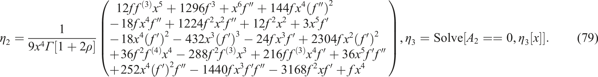
After substituting equations (66)–(68) into equation (69), we get

$D_t^{\rho }{\eta }_1=-c3x^8-c4x^{10}+x^2\left(c1x^2+c2x^4\right).$

(72)

Applying the inverse operator on equation (72) yields

${\eta }_1=x^4\left(c_1+c_2{x}^2-c_3{x}^4-c_4{x}^6\right)\frac{t^{\rho }}{\rho \Gamma \left[\rho \right]}.$

(73)

By collecting equations (67) and (73), the following OAFM solution is obtained

$\eta \left(x,\tau \right)={\eta }_0+{\eta }_1=x^2+x^4\left(c_1+c_2{x}^2-c_3{x}^4-c_4{x}^6\right)\frac{t^{\rho }}{\rho \Gamma \left[\rho \right]}.$

(74)

The Auxiliary constants for this example read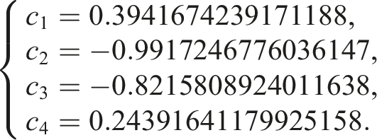

$\{\begin{array}{l}{c}_1=0.3941674239171188,\\ c_2=-0.9917246776036147,\\ c_3=-0.8215808924011638,\\ c_4=0.24391641179925158.\end{array}$

By inserting the obtained values of the auxiliary constants into equation (74), the following approximate solution to the problem (60) is obtained as follows

$\eta \left(x,\tau \right)=x^2+t\left(-0.991725x^2-0.243916x^6+0.821581x^4+0.394167\right)x^4.$

(75)

The Tantawy technique for analyzing example (3)

The Tantawy technique can be utilized to analyze example (3) by delineating the subsequent points:

Step (1): To solve and analyze the IVP (60), the following Ansatz is considered

$\eta =f+t^{\rho }{\eta }_1+t^{2\rho }{\eta }_2+t^{3\rho }{\eta }_3+\cdots ,$

(76)where ${\eta }_0\equiv f=x$ indicates the IC and ${\eta }_i\equiv {\eta }_i\left(x\right)$ for $i=1,2,3,\cdots ,$ are undetermined functions.

• Step (2): To determine the values of the unknown functions ${\eta }_i$ , we insert the Ansatz (76) into equation (60), which leads to the following result

$\frac{{\partial }^{\rho }}{\partial t^{\rho }}\left[f+t^{\rho }{\eta }_1+t^{2\rho }{\eta }_2+t^{3\rho }{\eta }_3+\cdots \right]=-{\partial }_x\left[\frac{4}{x}{\left(f+t^{\rho }{\eta }_1+t^{2\rho }{\eta }_2+t^{3\rho }{\eta }_3+\cdots \right)}^2\right]$

$+{\partial }_x\left[\frac{x}{3}\left(f+t^{\rho }{\eta }_1+t^{2\rho }{\eta }_2+t^{3\rho }{\eta }_3+\cdots \right)\right]+{\partial }_x^2\left[{\left(f+t^{\rho }{\eta }_1+t^{2\rho }{\eta }_2+t^{3\rho }{\eta }_3+\cdots \right)}^2\right].$

(77)

• Step (3): Collecting the coefficients of the same power of $t^{i\rho }$ and after using the definition of the CFDO, we get

$A_0+A_1{t}^{\rho }+A_2{t}^{2\rho }+\cdots =0,$

(78)with

$A_0=\Gamma \left[1+\rho \right]{\eta }_1-\frac{f}{3}-\frac{4f^2}{x^2}+\frac{8f{f}^{\prime }}{x}-\frac{x}{3}{f}^{\prime }-2{\left(f^{\prime }\right)}^2-2f{f}^{″},$

$A_1=\frac{\Gamma \left[1+2\rho \right]{\eta }_2}{\Gamma \left[1+\rho \right]}-\frac{{\eta }_1}{3}-\frac{8f{\eta }_1}{x^2}+\frac{8{\eta }_1{f}^{\prime }}{x}+\frac{8f{{\eta }_1}^{\prime }}{x}-\frac{x{{\eta }_1}^{\prime }}{3}-4f^{\prime }{{\eta }_1}^{\prime }-2{\eta }_1{f}^{″}-2f{{\eta }_1}^{″},$

$A_2=\frac{\Gamma \left[1+3\rho \right]{\eta }_3}{\Gamma \left[1+2\rho \right]}-\frac{4{\eta }_1^2}{x^2}-\frac{{\eta }_2}{3}-\frac{8f{\eta }_2}{x^2}+\frac{8f^{\prime }{\eta }_2}{x}+\frac{8{\eta }_1{{\eta }_1}^{\prime }}{x}-2{\left({{\eta }_1}^{\prime }\right)}^2+\frac{8f}{x}{{\eta }_2}^{\prime }-\frac{x}{3}{{\eta }_2}^{\prime }-4f^{\prime }{{\eta }_2}^{\prime }-2f^{″}{\eta }_2-2{\eta }_1{{\eta }_1}^{″}-2f{{\eta }_2}^{″},⋮.$

• Step (4): Equating to zero the coefficients $A_i$ for $i=0,1,2,$ and solving the obtained system in ${\eta }_i\equiv {\eta }_i\left(x\right)$ , we finally get the explicit values of ${\eta }_i\equiv {\eta }_i\left(x\right)$ as follows

${\eta }_1=\frac{1}{3x^2\Gamma \left[1+\rho \right]}\left(x^{2}f+12f^2-24xf{f}^{\prime }+x^3{f}^{\prime }+6x^2{\left(f^{\prime }\right)}^2+6x^{2}f{f}^{″}\right)$

${\eta }_2=\frac{1}{9x^4\Gamma \left[1+2\rho \right]}\left(\begin{array}{l} 12f{f}^{\left(3\right)}{x}^5+1296f^3+x^6{f}^{″}+144f{x}^4{\left(f^{″}\right)}^2\\ -18f{x}^4{f}^{″}+1224f^2{x}^2{f}^{″}+12f^2{x}^2+3x^5{f}^{\prime }\\ -18x^4{\left(f^{\prime }\right)}^2-432x^3{\left(f^{\prime }\right)}^3-24f{x}^3{f}^{\prime }+2304f{x}^2{\left(f^{\prime }\right)}^2\\ +36f^2{f}^{\left(4\right)}{x}^4-288f^2{f}^{\left(3\right)}{x}^3+216f{f}^{\left(3\right)}{x}^4{f}^{\prime }+36x^5{f}^{\prime }{f}^{″}\\ +252x^4{\left(f^{\prime }\right)}^2{f}^{″}-1440f{x}^3{f}^{\prime }{f}^{″}-3168f^{2}x{f}^{\prime }+f{x}^4\end{array}\right),{\eta }_3=\text{Solve}\left[A_2==0,{\eta }_3\left[x\right]\right].$

(79)For simplicity, we can use the MATHEMATICA command $\text{Solve}\left[A_2==0,{\eta }_3\left[x\right]\right]$ to find the value of ${\eta }_3$ . Note that we wrote the MATHEMATICA command here due to the huge size of ${\eta }_3.$

• Step (5): Inserting the value of the IC $f=x^2$ into equation (79), we finally get the values of ${\eta }_i$ as follows

${\eta }_1=\frac{x^2}{\Gamma \left[1+\rho \right]},{\eta }_2=\frac{x^2}{\Gamma \left[1+2\rho \right]},{\eta }_3=\frac{x^2}{\Gamma \left[1+3\rho \right]}.$

(80)

• Step (6): Inserting the obtained values of ${\eta }_i$ into the Ansatz (76), we finally get the exact solution for the suggested problem as follows

$\eta =x^2+\frac{x^2}{\Gamma \left[1+\rho \right]}{t}^{\rho }+\frac{x^2}{\Gamma \left[1+2\rho \right]}{t}^{2\rho }+\frac{x^2}{\Gamma \left[1+3\rho \right]}{t}^{3\rho }+\cdots .$

(81)

The residual error for this approximation reads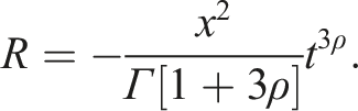

$R=-\frac{x^2}{\Gamma \left[1+3\rho \right]}{t}^{3\rho }.$

Utilizing Laplace HPM (LHPM) and following extensive computations and significant time expenditure, we obtain findings identical to those produced by the Tantawy technique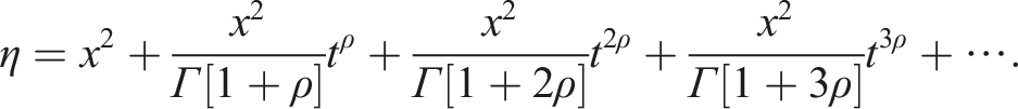

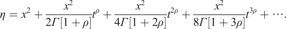
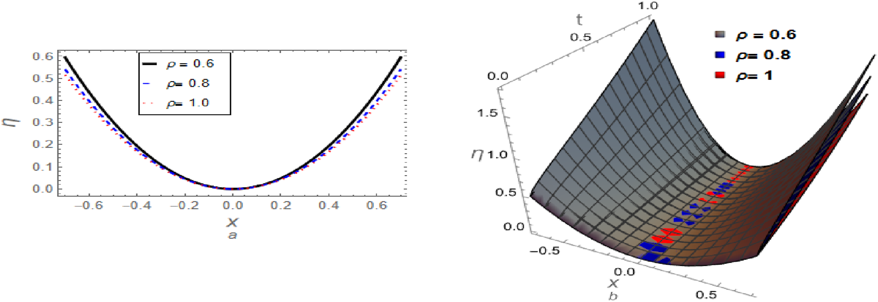
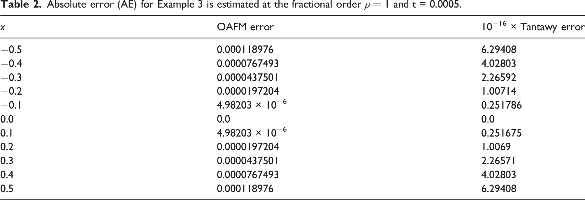
$\eta =x^2+\frac{x^2}{\Gamma \left[1+\rho \right]}{t}^{\rho }+\frac{x^2}{\Gamma \left[1+2\rho \right]}{t}^{2\rho }+\frac{x^2}{\Gamma \left[1+3\rho \right]}{t}^{3\rho }+\cdots .$

Both the approximation (75) using OAFM and the approximation (81) using Tantawy technique are graphically analyzed for different values to the fractional order parameter $\rho$ , as illustrated in Figures 9 and 10, respectively. Furthermore, as illustrated in Figure 11(a) and (b)), respectively, we conducted a numerical comparison between the generated approximations and the exact solution for the integer case at both short and long time intervals. We additionally calculated the absolute error for both approximations (75) and (81), as presented in Table 2.

Figure 9.

The behavior of fractional approximation (75) using OAFM at various values of fractional order parameter for Example (3) (a) two-dimensional graph and (b) three-dimensional graph.

Figure 10.

The behavior of fractional approximation (81) using Tantawy technique at various values of fractional order parameter for Example (3) (a) two-dimensional graph and (b) three-dimensional graph.

Figure 11.

A comparison between the derived approximations (75) and (81) with the exact solution (62) for the integer case: (a) at a short time and (b) at a long time.

Table 2.

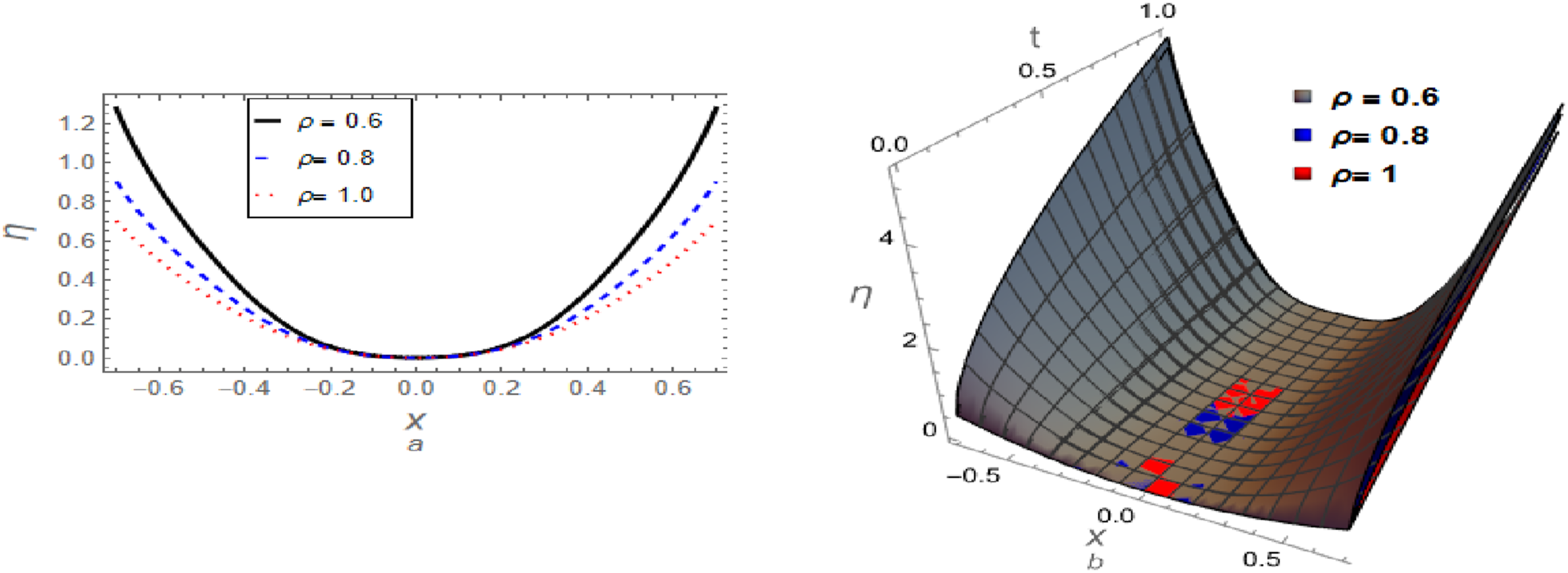
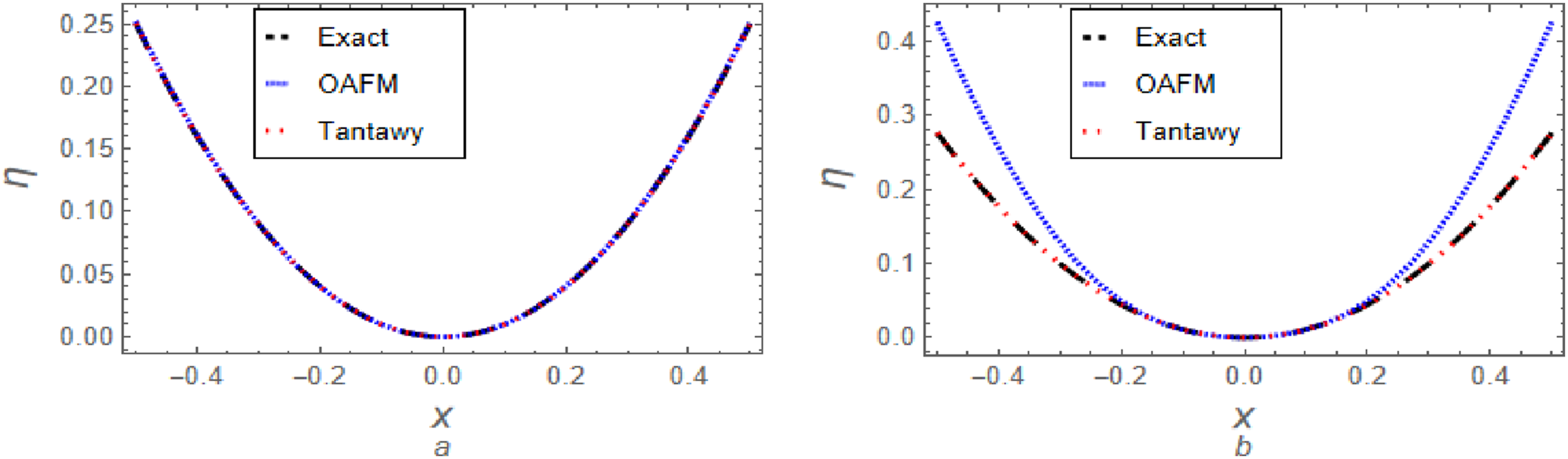
Absolute error (AE) for Example 3 is estimated at the fractional order $\rho =1$ and t = 0.0005.

$x$	OAFM error	10−16 × Tantawy error
−0.5	0.000118976	6.29408
−0.4	0.0000767493	4.02803
−0.3	0.0000437501	2.26592
−0.2	0.0000197204	1.00714
−0.1	4.98203 × 10−6	0.251786
0.0	0.0	0.0
0.1	4.98203 × 10−6	0.251675
0.2	0.0000197204	1.0069
0.3	0.0000437501	2.26571
0.4	0.0000767493	4.02803
0.5	0.000118976	6.29408

The comparison results showed the high accuracy and efficiency of the derived approximations, which enhances the efficiency of the proposed methods. However, it is essential to highlight the innovation of the Tantawy technique. The numerical analysis proved that the Tantawy technique is more accurate throughout the whole study domain and significantly outperforms OAFM. Future studies anticipate this technique to be the most popular among various analysis methods due to its simplicity in calculation, efficiency, and high stability, leading to the derivation of more accurate approximations and the provision of closed solutions for exact solutions.

Conclusion

In this investigation, a novel technique, the “Tantawy technique,” has been implemented for analyzing the fractional Fokker–Planck (FFP) equations, in addition to the optimal auxiliary function method (OAFM) in the framework of the Caputo operator. Since Tantawy’s technique was mentioned for the first time in this investigation, we have provided a simplified explanation to enable the reader to comprehend and apply it to any new model. The two methods have been used to three distinct models of the FFP equation, each exhibiting different levels of complexity, to study them and derive highly accurate approximations that simulate the nonlinear phenomena described by these models. All derived approximations of the three models utilizing the two proposed methods have been graphically and numerically investigated. This analysis included two-dimensional and three-dimensional graphical representations to elucidate the dynamics of the nonlinear phenomena described by these models and assess the fractional parameter’s influence on their behavior. Additionally, we estimated the absolute error of all derived approximations compared to the exact solutions as the benchmark for the integer cases to evaluate the correctness of these approximations. Also, we conducted a graphical and numerical comparison of the resulting approximations to assess the efficacy of each method individually. It was found that both approaches yield favorable results in the limited research domain, but in arbitrary/large domains, Tantawy’s technique is distinctly superior to OAFM in terms of accuracy and stability. This, in turn, promises good results and enhances Tantawy’s technique in analyzing various physical and engineering problems and other problems related to studying the equations of ascension in their fractional forms.

Moreover, the Tantawy technique, developed for the first time, has effectively analyzed the most complicated problems. It is distinguished by its extreme simplicity, high accuracy, and stability throughout the whole study domain, which is not attained by many other methods. Additionally, it generated more accurate and stable approximations than many other similar methods. We anticipate that the Tantawy approach, given the current study and its remarkable outcomes, will emerge as the most favored and popular method among its counterparts in future studies.

While the Tantawy technique yields results comparable to LHPM, it is more adaptable, efficient, and uncomplicated than LHPM. Furthermore, unlike alternative methods, it does not necessitate any complexities. Moreover, calculations require less time than other laborious and time-intensive approaches.

Future work

• Considering the physical and engineering significance of the models analyzed through the “Tantawy technique,” these models may also be examined using various other methodologies that have demonstrated their efficacy in addressing diverse physical and engineering challenges, such as homotopy perturbation-type techniques,^33–36 the Elzaki decomposition method (DM), ³⁷ the variational iteration method, ³⁸ the Laplace transform DM, ³⁹ the residual power series method (RSPM), and the new iteration method (NIM)^40–44, as these methods are anticipated to yield more precise approximate solutions in comparison to numerous alternative approaches.

• In future studies, researchers might compare the approximations made by other methods with those made by the Tantawy technique to determine how reliable and helpful this new method is. Furthermore, Tantawy’s technique can be used to analyze various (non)-integrable fractional plasma wave equations, such as the family of third-order fractional KdV-type equations,^45–49 the family of fifth-order fractional KdV-type equations,^50–55 the family of fractional nonlinear Schrödinger-type equations,^56–60 to understand the behavior and propagation dynamics of nonlinear phenomena arising in multi-plasma systems. The Tantawy technique is also expected to successfully analyze fractional ordinary differential equations such as different fractional pendulum oscillators.^61,62

• Since this is the first core of the Tantawy technique, which we integrated with the Caputo operator to analyze the problem under study, it is anticipated that this technique will be applicable with several additional operators, including the two-scale fractal derivative and He’s fractional derivative.^63–67