Novel approximations to the fourth-order fractional Cahn–Hillard equations: Application to the Tantawy Technique and other two techniques with Yang transform

Abstract

This investigation employs the “Tantawy Technique,” a novel, highly accurate, and fast technique, to solve and analyze the fourth-order time-fractional Cahn–Hilliard (TFCH) models. We also implement the variational iteration transform method (VITM) and the homotopy perturbation transform method (HPTM) within the Yang transform framework to analyze the fourth-order TFCH models. These iterative procedures enable the acquisition of solutions in a convergent series. We focus on two nonlinear issues in the current investigation to demonstrate the validity and accuracy of the suggested approaches. We check the derived approximations against the exact solutions for the integer cases and then find their absolute error to ensure their accuracy and stability. The present approaches show how different fractional orders affect the profile of the derived approximations. The presented issues demonstrate the precision and effectiveness of the suggested techniques in tackling strong nonlinear fractional differential equations. Implementing the suggested methodologies indicates that as the value of the fractional parameter transitions from fractional to integer order, the result approaches the exact solution for the integer case. These methods also make it straightforward to use fractal calculus in real life. The numerical analysis results demonstrate that the proposed iterative techniques are viable and user-friendly tools with high computational efficiency when used in various physical models in science and engineering.

Introduction

Conventional derivative equations cannot adequately capture many real-world problems. Ultimately, fractional derivative-related problems have attracted the attention of numerous academics. Fractional calculus is a crucial part of calculus because of its applications in fractional order integration and differentiation. Fractional calculus (FC) is not a novel concept. It handles ordinary differentiation and integration of arbitrary order and modifies classical calculus. It dates back to a late seventeenth-century letter written by Leibniz to L’Hospital. The fundamental principle of fractional calculus is that fractional operators, not integer operators, are used to model natural occurrences. Therefore, FC focuses on characteristics that conventional theory cannot model.^1–4 Riemann–Liouville and Liouville–Caputo are the two primary types of fractional derivatives. From time to time, new definitions of fractional operators and integrals are provided. These modifications of the Liouville–Caputo operator add extra previously unavailable characteristics and are necessary for advancing fractional calculus theory. Therefore, fractional calculus has proven to be an effective tool for researching applied science-related subjects. FC has seen significant application in recent years. FC has been used to study various linear and nonlinear phenomena.^5,6 A few domains that employ fractional order modeling are education, ⁷ agriculture, ⁸ ocean waves, ⁹ health, ¹⁰ robotics, ¹¹ and construction. ¹²

Many researchers in the applied sciences and engineering have become interested in the study of fractional partial differential equations (FPDEs) because of their numerous applications in a variety of fields, including the theory of long-range interaction, ¹³ mechanics of non-Hamiltonian systems, ¹⁴ physical kinetics, ¹⁵ mechanics of fractional media, ¹⁶ and other areas.^17–19 Fractional differential equation models have many physical applications in science and engineering and are very helpful for various physical challenges. Due to the operator’s integral definition, solving partial differential equations with fractional derivatives is frequently more challenging than solving classical equations. Regardless of their order, the solutions to these nonlinear FDEs are essential for describing the characteristics and behavior of complicated issues in applied mathematics and technology. Many efforts have been made to establish effective strategies for solving FPDEs, but it’s important to remember that obtaining an analytical or approximate solution can be difficult. As a result, accurate strategies for solving FPDEs are currently being researched. The primary distinction between the analytical and numerical approaches is that the numerical method delivers the result at discrete points. In contrast, the analytical technique provides the solution as a continuous graph. The literature contains several analytical and numerical techniques for resolving FPDEs, such as Generalized differential transform method, ²⁰ Yang transform decomposition method,^21,22 Laplace Residual Power Series Method, ²³ q-homotopy analysis generalized transform method, ²⁴ Jacobi operational matrix scheme, ²⁵ Elzaki transform decomposition method,^26,27 Homotopy perturbation transform method, ²⁸ and so on.

Using nonlinear partial differential equations (NPDEs) is essential in many engineering and natural sciences branches. We have the Cahn–Hillard (CH) equation among these NPDEs, called after Cahn and Hilliard in 1958. ²⁹ This equation is essential for explaining several interesting scientific phenomena, such as phase ordering dynamics and spinodal decomposition. Additionally, it discusses a crucial qualitative characteristic that sets apart two-phase systems and is related to phase separation procedures. Its fundamental characteristic is that the interface between the two phases is not sharp. However, it has a limited thickness, and the composition gradually changes. The equation is, therefore, considered to describe the temporal evolution of conserved fields. Berti and Bochicchio ³⁰ generalize the mathematical model representing a phase separation in the CH theory. Researchers have looked into this equation’s mathematical and numerical solutions because of its practical applicability in the many domains mentioned above.^31–36 Within this context, we examine the time-fractional CH (TFCH) equation:

$D_t^p\mathbf{J}=\kappa \frac{\partial \mathbf{J}}{\partial x}+6\mathbf{J}{\left(\frac{\partial \mathbf{J}}{\partial x}\right)}^2+3{\mathbf{J}}^2\frac{{\partial }^2\mathbf{J}}{\partial x^2}-\frac{{\partial }^2\mathbf{J}}{\partial x^2}-\frac{{\partial }^4\mathbf{J}}{\partial x^4},$

(1)

where $\mathbf{J}\equiv \mathbf{J}\left(x,t\right)$ , $D_t^p\equiv {\partial }^p/\partial t^p\equiv {\partial }_{t^p}^p$ indicates the order of the fractional derivative with $0<p\le 1$ and the parameter κ ≥ 0.

So one of the goals of this work is to use the variational iteration transform method (VITM) and Homotopy perturbation transform method (HPTM) to generate high accurate approximations in the form of recurrence relations. It is known that the variational iteration method (VIM) was invented by He and it was used effectively to solve autonomous ODEs.^37,38 For instance, the governing equations for the nonlinear oscillations of tapered beams were solved and examined utilizing the Aboodh transform-based VIM (ATVIM). ³⁹ He’s team found that the ATVIM yields results that necessitate less computational effort than other analytical methods and that a single iteration suffices to attain appropriate conclusions.

The VIM is acknowledged as an efficient technique for solving and analyzing various types of (non)linear and complicated DEs.^40–43 One of the most appealing aspects of the VIM compared to other analytical approaches is the absence of the need to linearize or solve nonlinear terms. Utilizing a suitable initial guess and incorporating Lagrange multipliers enables the acquisition of exact solutions for both linear and nonlinear issues. Nonetheless, identifying the multiplier is challenging without an understanding of the elusive theory of variational calculus. ⁴⁴ The VIM is pivotal in MEMS (micro-electro-mechanical systems). This approach allows for the precise analysis and modeling of the intricate behavior exhibited by MEMS devices. This method facilitates comprehension of the dynamic responses of MEMS structures, including vibrations and deformations. Providing analytical approximations enables engineers to optimize the design of MEMS components for enhanced performance and reliability. Furthermore, it can handle nonlinearities commonly found in MEMS systems, thereby providing more accurate predictions than traditional methods. In conclusion, it can be stated that this method is a valuable tool for the development and improvement of MEMS technology.^45–49

He initially introduced the homotopy perturbation method (HPM) in 1998, ⁵⁰ and it was later improved and refined by many authors.^51–54 This method provides an approximate solution as a quickly convergent series approaching the exact results. Many subsequent studies have shown that this method and its family perform well in handling various linear and nonlinear problems. From this standpoint, many researchers used this approach and its family to analyze various types of differential equations and derive accurate approximations that accurately simulate natural phenomena. For example, Odibat and Momani ⁵⁵ demonstrated the significance of HPM in many fields and showed that the HPM has an excellent treatment in providing the exact solution to various differential equations (DEs). Likewise, the Yang transform (YT) was introduced to modify several techniques, such as the VIM and HPM. After applying YT, these techniques become called VITM and HPTM. The VITM was utilized to solve several kinds of DEs (ordinary and partial DEs). For instance, in Ref. 56, the authors used the VIM with Laplace transform to solve linear fractional DEs (FDEs). The authors found that the modified method is more efficient than other versions of the VIM in analyzing fractional DEs. In Ref. 57, the authors utilized the Laplace transform to ascertain the Lagrange multiplier readily. They also used the hybrid VITM to analyze a nonlinear oscillatory equation and obtained a result similar to the normal HPM ⁵⁸ and He’s frequency–amplitude formulation. ⁵⁹ The VITM surpasses Adomian’s decomposition method by resolving the issue without requiring the computation of Adomian’s polynomials. Recently, many authors studied the HPT with novel transforms for solving FPDEs such as time-fractional diffusion problems, ⁶⁰ time-fractional Korteweg-de Vries equation, ⁶¹ and fractional Kaup–Kupershmidt equation. ⁶² This attempt presents two novel techniques (VITM and HPTM) for solving TFCH equations with few and successive steps, which makes it unique. For the first time, we will also introduce a newly established approach for studying all sorts of fractional differential equations, the Tantawy Technique, created by Samir El-Tantawy in early December 2024. ⁶³ After that, we will elucidate in detail how to apply this technique in analyzing various fractional differential equations.

The following overview of the article’s main content: The primary definitions and a few more ideas for understanding fractional differential equations are included in Section 2. Section 3 discusses the Tantawy Technique and comprehensively explains how to apply it to analyze different differential equations. Also, section 4 outlines the basic strategy of VITM for addressing the given issues. Additionally, section 5 outlines the basic strategy of HPTM for addressing the problems given. The convergence analysis of the suggested methods is discussed in Section 6 of the manuscript. Section 7 considers some numerical examples, and all suggested methods are applied for analyzing these problems and deriving highly accurate approximations for the TFCH equations. We present our conclusion in Section 8.

Basic definitions

This section discusses several notable definitions pertinent to our current project.

Definition 1

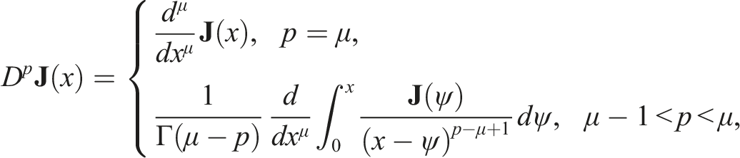
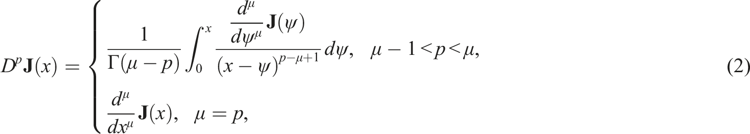
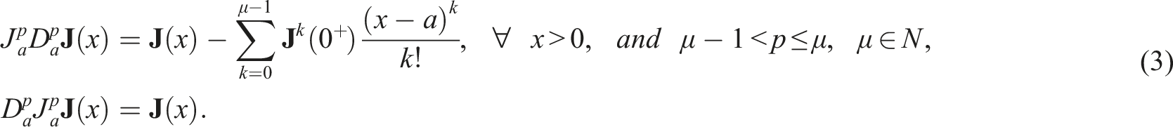
The Riemann-Liouville’s (RL) non-integer derivative operator is expressed as ⁶⁴

$D^p\mathbf{J}(x)=\left\{\begin{array}{c}\frac{d^{\mu }}{d{x}^{\mu }}\mathbf{J}(x),p=\mu ,\hfill \\ \frac{1}{\mathrm{\Gamma }(\mu -p)}\frac{d}{d{x}^{\mu }}{\int }_0^x\frac{\mathbf{J}(\psi )}{{(x-\psi )}^{p-\mu +1}}d\psi ,\mu -1<p<\mu ,\hfill \end{array}\right.$

with μ ∈ Z⁺, p ∈ R⁺.

Definition 2

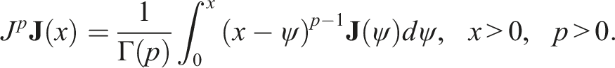
The fractional RL integral operator of order p ∀ p ≥ 0, of the function J(x) is expressed as

$J^p\mathbf{J}(x)=\frac{1}{\mathrm{\Gamma }(p)}{\int }_0^x{(x-\psi )}^{p-1}\mathbf{J}(\psi )d\psi ,x>0,p>0.$

with properties

$\left\{\begin{array}{c}\hfill J^p{x}^{\mu }=\frac{\mathrm{\Gamma }\left[\mu +1\right]}{\mathrm{\Gamma }\left[\mu +p+1\right]}{x}^{\mu +p},\hfill \\ \hfill D^p{x}^{\mu }=\frac{\mathrm{\Gamma }\left[\mu +1\right]}{\mathrm{\Gamma }\left[\mu -p+1\right]}{x}^{\mu -p}.\hfill \end{array}\right.$

Definition 3

The fractional Caputo derivative operator (CDO) of order p to the function J(x) is expressed as ⁶⁵

$D^p\mathbf{J}(x)=\left\{\begin{array}{c}\frac{1}{\mathrm{\Gamma }(\mu -p)}{\int }_0^x\frac{\frac{d^{\mu }}{d{\psi }^{\mu }}\mathbf{J}(\psi )}{{(x-\psi )}^{p-\mu +1}}d\psi ,\mu -1<p<\mu ,\hfill \\ \frac{d^{\mu }}{d{x}^{\mu }}\mathbf{J}(x),\mu =p,\hfill \end{array}\right.$

(2)

with properties

$\begin{array}{cc}\hfill J_a^p{D}_a^p\mathbf{J}(x)& =\mathbf{J}(x)-\sum _{k=0}^{\mu -1}{\mathbf{J}}^k(0^{+})\frac{{\left(x-a\right)}^k}{k!},\forall x>0,and\mu -1<p\le \mu ,\mu \in N,\hfill \\ \hfill D_a^p{J}_a^p\mathbf{J}(x)& =\mathbf{J}(x).\hfill \end{array}$

(3)

Definition 4

He’s fractional derivative is stated as ⁶⁶ :

$D_t^p\mathbf{J}=\frac{1}{\mathrm{\Gamma }(n-p)}\frac{d^n}{d{t}^n}{\int }_{t_0}^t{(s-t)}^{n-p-1}[{\mathbf{J}}_0(s)-\mathbf{J}(s)]ds,$

(4)

where J₀(s) is a known function.

Definition 5

The Yang transform (YT) of the function J(t) is stated as^67,68

$Y\left[\mathbf{J}(t)\right]\equiv Y\left[\mathbf{J}(t),u\right]=\mathcal{R}(u)={\int }_0^{\infty }{e}^{\frac{-t}{u}}\mathbf{J}(t)dt,t>0,$

(5)

where u indicates the transform variable. Also, the inverse YT reads

$Y^{-1}\left[\mathcal{R}(u)\right]=\mathbf{J}(t).$

(6)

Definition 6

The YT of fractional derivative is stated as ^67,68

$Y\left[D^p\mathbf{J}(t)\right]=\frac{\mathcal{R}(u)}{u^p}-\sum _{k=0}^{n-1}\frac{{\mathbf{J}}^{\left(k\right)}(0)}{u^{p-(k+1)}},0<p\le n.$

(7)

Definition 7

The YT of the function J ≡ J(x, t) is stated as ⁶⁴

$Y\left[\mathbf{J}(x,t)\right]\equiv Y\left[\mathbf{J}(x,t),u\right]=\mathcal{R}(x,u)={\int }_0^{\infty }{e}^{\frac{-t}{u}}\mathbf{J}(x,t)dt,t>0.$

(8)

Definition 8

The YT of the fractional CDO of order p to the function J ≡ J(x, t) with regard to t is expressed as follows ⁶⁴ :

$Y\left[D_t^p\mathbf{J}\right]\equiv Y\left[D_t^p\mathbf{J};u\right]=\frac{\mathcal{R}(x,u)}{u^p}-\sum _{k=0}^{n-1}{u}^{k-p+1}{\mathbf{J}}^{\left(k\right)}\left(x,0\right){|}_{t=0}.$

(9)

Brief description of the Tantawy Technique

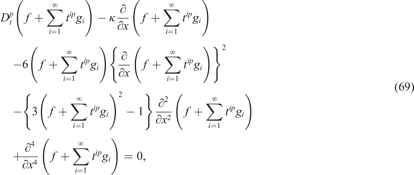
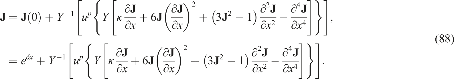
Tantawy’s technique is a novel method developed by Samir El-Tantawy in December 2024. ⁶³ This technique is significantly more efficient than alternative methods, as it is not computationally intensive and does not require an extended duration to compute higher approximations. In contrast, the HPM may necessitate considerable time to achieve similar higher approximations. Furthermore, this technique is straightforward and can readily be employed by novice researchers to solve and analyze any fractional differential (non)linear equation to expedite higher order approximations. Also, it is devoid of the complications that are typically associated with alternative methods. The technique can be articulated more straightforwardly through the subsequent key points:

Step (1) Let us first present the following fractional differential equation

$D_t^p\mathbf{J}=Q\left[x,t,{\mathbf{J},\mathit{\partial }}_x{\mathbf{J},\mathit{\partial }}_x^2{\mathbf{J},\mathit{\partial }}_x^3\mathbf{J},\cdots \right],$

(10)

with the initial solution/initial condition (IC)

$\mathbf{J}(x,0)\equiv {\mathbf{J}}_0=f,$

(11)

where J ≡ J(x, t), Q is a polynomial in J and its derivatives and $f\equiv f\left(x\right)$ . It should also be noted that this method is not limited to analyzing one-dimensional fractional equations only but can also be applied to multidimensional fractional equations.

• Step (2) Inserting the following Ansatz

$\mathbf{J}=f+\sum _{i=1}^{\infty }{t}^{ip}{g}_i=f+t^p{g}_1+t^{2p}{g}_2+t^{3p}{g}_3+\cdots +t^{np}{g}_n+\cdots ,$

(12)

into equation (10) implies

$D_t^p\left[f+\sum _{i=1}^{\infty }{t}^{ip}{g}_i\right]=Q\left[\begin{array}{c}\hfill x,t,\left(f+\sum _{i=1}^{\infty }{t}^{ip}{g}_i\right){,\mathit{\partial }}_x\left(f+\sum _{i=1}^{\infty }{t}^{ip}{g}_i\right),\hfill \\ \hfill {\mathit{\partial }}_x^2\left(f+\sum _{i=1}^{\infty }{t}^{ip}{g}_i\right),\cdots \hfill \end{array}\right]$

(13)

where $g_i\equiv g_i\left(x\right)$ are unknown functions, which will be determined later.

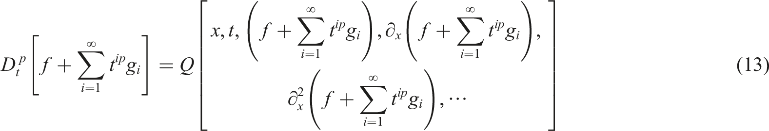
Step (3) According to solution (12), the fractional CDO $D_t^p\mathbf{J}$ to the function J can be written in the following manner

$D_t^p\mathbf{J}=\sum _{i=1}^{\infty }{g}_i{D}_t^p\left[t^{ip}\right]=\sum _{i=1}^{\infty }{g}_i\frac{\mathrm{\Gamma }\left[ip+1\right]}{\mathrm{\Gamma }\left[(i-1)p+1\right]}{t}^{(i-1)p},$

(14)

where $\mathrm{\Gamma }\left(n+1\right)=n!$ indicates gamma function and i = 1, 2, 3, ⋯ .

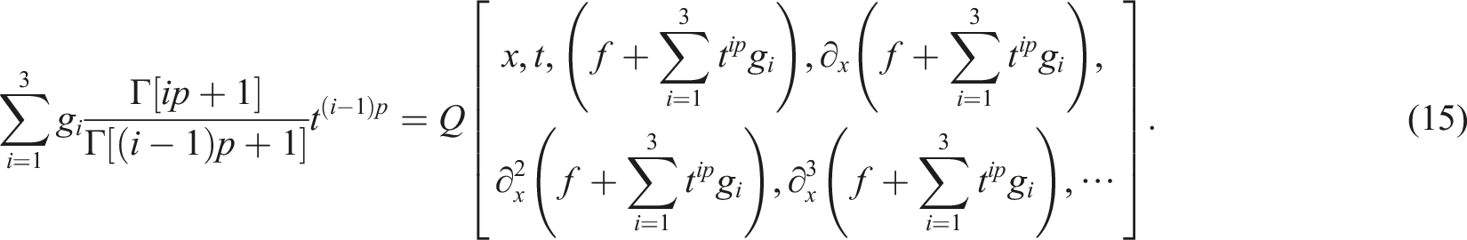
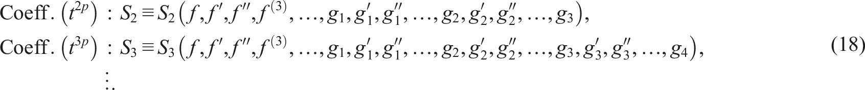
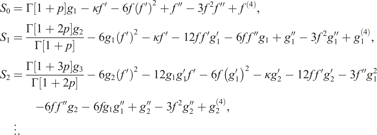
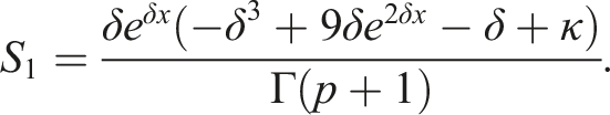
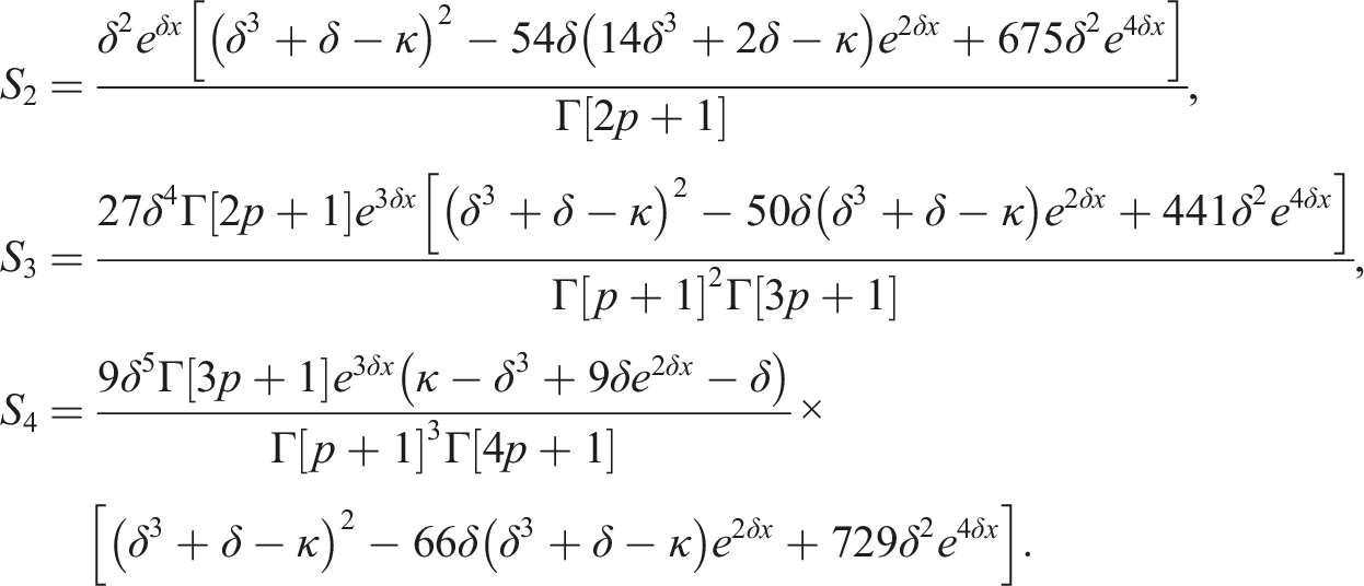
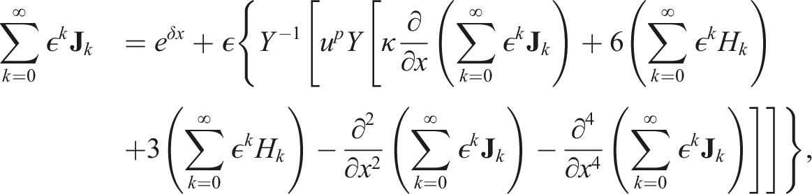
Step (4) For a certain number n ^th in the series solution (say n = 3) and by using equation (14) then equation (13) becomes

$\sum _{i=1}^3{g}_i\frac{\mathrm{\Gamma }\left[ip+1\right]}{\mathrm{\Gamma }\left[(i-1)p+1\right]}{t}^{(i-1)p}=Q\left[\begin{array}{c}\hfill x,t,\left(f+\sum _{i=1}^3{t}^{ip}{g}_i\right){,\mathit{\partial }}_x\left(f+\sum _{i=1}^3{t}^{ip}{g}_i\right),\hfill \\ \hfill {\mathit{\partial }}_x^2\left(f+\sum _{i=1}^3{t}^{ip}{g}_i\right),{\partial }_x^3\left(f+\sum _{i=1}^3{t}^{ip}{g}_i\right),\cdots \hfill \end{array}\right].$

(15)

• Step (5) Now, by aggregating all terms associated with identical powers of t ^ip ∀ i = 0, 1, 2, 3, …, we obtain

$\sum _{i=0}{S}_i{t}^{ip}=S_0+S_1{t}^p+S_2{t}^{2p}+S_3{t}^{3p}+\cdots =0,$

(16)

with

$\begin{array}{ll}\hfill \text{Coeff.\hspace{0.17em}}\left(t^{0p}\right)& :\hspace{0.17em}{S}_0\equiv S_0\left(f,f^{\prime },f^{\prime \prime },f^{\left(3\right)},\dots ,g_1\right),\hfill \\ \hfill \text{Coeff.\hspace{0.17em}}\left(t^{1p}\right)& :\hspace{0.17em}{S}_1\equiv S_1\left(f,f^{\prime },f^{\prime \prime },f^{\left(3\right)},\dots ,g_1,g_1^{\prime },g_1^{\prime \prime },\dots ,g_2\right),\hfill \end{array}$

(17)

$\begin{array}{ll}\hfill \text{Coeff.\hspace{0.17em}}\left(t^{2p}\right)& :\hspace{0.17em}{S}_2\equiv S_2\left(f,f^{\prime },f^{\prime \prime },f^{\left(3\right)},\dots ,g_1,g_1^{\prime },g_1^{\prime \prime },\dots ,g_2,g_2^{\prime },g_2^{\prime \prime },\dots ,g_3\right),\hfill \\ \hfill \text{Coeff.\hspace{0.17em}}\left(t^{3p}\right)& :\hspace{0.17em}{S}_3\equiv S_3\left(f,f^{\prime },f^{\prime \prime },f^{\left(3\right)},\dots ,g_1,g_1^{\prime },g_1^{\prime \prime },\dots ,g_2,g_2^{\prime },g_2^{\prime \prime },\dots ,g_3,g_3^{\prime },g_3^{\prime \prime },\dots ,g_4\right),\hfill \\ \hfill & ⋮.\hfill \end{array}$

(18)

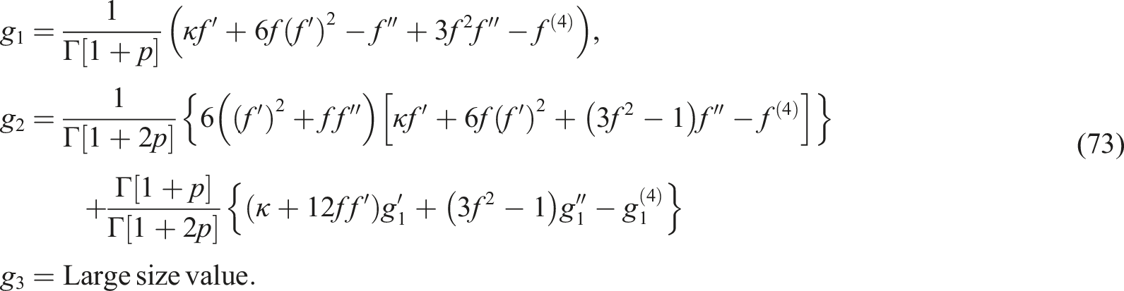
• Step (6) By setting the coefficients S _i ∀ i = 0, 1, 2, 3, …, to zero, we obtain a system of equations. Solving this system for g₁, g₂, g₃, …, yields implicit expressions for g _i as functions of the IC f and its derivatives as follows

$\begin{array}{ll}\hfill g_1& =\left(H_1\left(p\right),f,f^{\prime },f^{\prime \prime },g^{\left(3\right)},\dots \right),\hfill \\ \hfill g_2& =\left(H_2\left(p\right),f,f^{\prime },f^{\prime \prime },f^{\left(3\right)},\dots ,g_1,g_1^{\prime },g_1^{\prime \prime },\dots \right),\hfill \\ \hfill g_3& =\left(H_3\left(p\right),f,f^{\prime },f^{\prime \prime },f^{\left(3\right)},\dots ,g_1,g_1^{\prime },g_1^{\prime \prime },\dots ,g_2,g_2^{\prime },g_2^{\prime \prime },\dots \right),\hfill \\ \hfill g_4& =\left(H_3\left(p\right),f,f^{\prime },f^{\prime \prime },f^{\left(3\right)},\dots ,g_1,g_1^{\prime },g_1^{\prime \prime },\dots ,g_2,g_2^{\prime },g_2^{\prime \prime },\dots ,g_3,g_3^{\prime },g_3^{\prime \prime },\dots \right),\hfill \\ \hfill & ⋮,\hfill \end{array}$

(19)

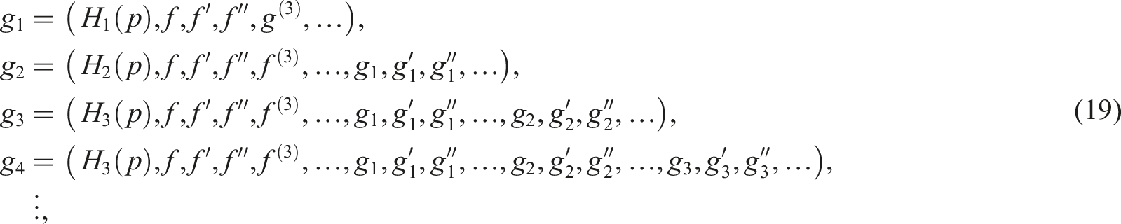
where the known functions $H_i\left(p\right)$ appeared after applying the fractional CDO.

Step (7) By utilizing the explicit value of the IC f in equation (19), we may derive the explicit values for g _i . By putting the obtained values of g _i into equation (12), we ultimately derive the approximate solution to the problem (10).

Brief description of the VITM

Here, we present the general description of the VITM. Consider the general nonlinear FPDE of the form

$\begin{array}{c}\hfill D_t^p\mathbf{J}+{\mathcal{P}}_1+{\mathcal{Q}}_1-{\mathcal{G}}_1=0,m-1<p\le m,\hfill \end{array}$

(20)

with

$\mathbf{J}(x,0)={\mathbf{J}}_0,$

(21)

where J ≡ J(x, t) and $D_t^p={\partial }^p/\partial t^p$ indicates the fractional CDO of order p. Here, ${\mathcal{P}}_1\equiv {\mathcal{P}}_1\left(\mathbf{J}\right)$ and ${\mathcal{Q}}_1\equiv {\mathcal{Q}}_1\left(\mathbf{J}\right)$ are linear and nonlinear operators, respectively, and ${\mathcal{G}}_1\equiv {\mathcal{G}}_1\left(x,t\right)$ is a source term.By employing YT to (20)

$Y[D_t^p\mathbf{J}]+Y[{\mathcal{P}}_1+{\mathcal{Q}}_1-{\mathcal{G}}_1]=0,$

(22)

where $Y[D_t^p\mathbf{J}]\equiv Y[D_t^p\mathbf{J}\left(x,t\right),u]$ .

Implementing the YT differentiation property, we obtain

$Y\left[\mathbf{J}\right]-\sum _{k=0}^{n-1}\frac{1}{u^{p-k-1}}{\mathbf{J}}^{\left(k\right)}{|}_{t=0}=-Y\left[{\mathcal{P}}_1+{\mathcal{Q}}_1-{\mathcal{G}}_1\right],$

(23)

where $Y\left[\mathbf{J}\right]=\mathcal{R}(x,u)/u^p$ and ${\mathbf{J}}^{\left(k\right)}\equiv {\partial }_t^k\mathbf{J}$ .

The iterative process for equation (23) is stated as

$$\begin{gathered} Y\left[{\mathbf{J}}_{m+1}\right]=Y\left[{\mathbf{J}}_m\right]+\lambda \left(u\right)\left\{\left(\frac{1}{u^p}Y\left[J_m\right]-\sum _{k=0}^{n-1}\frac{1}{u^{p-k-1}}{\mathbf{J}}^{\left(k\right)}{|}_{t=0}\right)+Y\left[{\mathcal{P}}_1+{\mathcal{Q}}_1-{\mathcal{G}}_1\right]\right\} \\ =\lambda \left(u\right)\left\{\left(-\sum _{k=0}^{n-1}\frac{1}{u^{p-k-1}}{\mathbf{J}}^{\left(k\right)}{|}_{t=0}\right)+Y\left[{\mathcal{P}}_1+{\mathcal{Q}}_1-{\mathcal{G}}_1\right]\right\}, \end{gathered}$$

(24)

with the following Lagrange multiplier

$\lambda (u)=-u^p,$

(25)

where ${\mathbf{J}}_m\equiv {\mathbf{J}}_m\left(x,t\right)$ and ${\mathbf{J}}_{m+1}\equiv {\mathbf{J}}_{m+1}\left(x,t\right)$ .

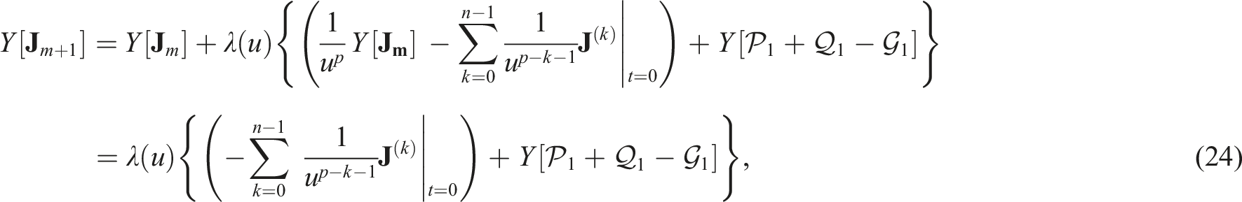
By applying inverse YT (Y⁻¹) on equation (24), we get

${\mathbf{J}}_{m+1}=Y^{-1}\left[u^p\left(\sum _{k=0}^{n-1}\frac{1}{u^{p-k-1}}{\mathbf{J}}^{\left(k\right)}{|}_{t=0}\mathbf{-}Y\left[{\mathcal{P}}_1+{\mathcal{Q}}_1-{\mathcal{G}}_1\right]\right)\right],$

(26)

and the initial iteration is illustrated as

${\mathbf{J}}_0(x,t)=Y^{-1}\left[u^p\left\{\sum _{k=0}^{n-1}\frac{1}{u^{p-k-1}}{\mathbf{J}}^{\left(k\right)}{|}_{t=0}\right\}\right].$

(27)

General procedure of the HPTM

To demonstrate the basic idea of the HPTM, we first introduce the following FPDE

$D_t^p\mathbf{J}={\mathcal{P}}_1+{\mathcal{Q}}_1,0<p\le 1,$

(28)

with the initial guess

$\mathbf{J}(x,0)\equiv {\mathbf{J}}_0=\theta (x).$

Here, $D_t^p={\partial }^p/\partial t^p$ denote the fractional CDO of order p, whereas ${\mathcal{P}}_1\equiv {\mathrm{P}}_1\left(\mathbf{J}\right)$ and ${\mathcal{Q}}_1\equiv {\mathcal{Q}}_1\left(\mathbf{J}\right)$ are, respectively, linear and nonlinear operators.

By applying the YT on equation (28), we have

$Y[D_t^p\mathbf{J}]=Y\left[{\mathcal{P}}_1+{\mathcal{Q}}_1\right],$

(29)

which leads to

$\frac{1}{u^p}\{\mathcal{R}(u)-u\mathbf{J}(0)\}=Y\left[{\mathcal{P}}_1+{\mathcal{Q}}_1\right].$

(30)

Accordingly, we get

$\mathcal{R}(u)=u\mathbf{J}(0)+u^{p}Y\left[{\mathcal{P}}_1+{\mathcal{Q}}_1\right].$

(31)

Operating inverse YT on equation (31), we have

$\mathbf{J}=\mathbf{J}(0)+Y^{-1}\left[u^{p}Y\left[{\mathcal{P}}_1+{\mathcal{Q}}_1\right]\right].$

(32)

In terms of HPM, we get ⁵³

$\mathbf{J}=\mathbf{J}(0)+ϵ\left(Y^{-1}\left[u^{p}Y\left[{\mathcal{P}}_1+{\mathcal{Q}}_1\right]\right]\right),$

(33)

with parameter ϵ ∈ [0, 1].The series form solution of unknown function reads

$\mathbf{J}=\sum _{k=0}^{\infty }{ϵ}^k{\mathbf{J}}_k,$

(34)

with

${\mathcal{Q}}_1=\sum _{k=0}^{\infty }{ϵ}^k{H}_k(\mathbf{J}),$

(35)

where J _k ≡ J _k (x, t) and H _k (J) indicates He’s polynomials, which can be operated as follows ⁵⁴

$H_k({\mathbf{J}}_0,{\mathbf{J}}_1,\dots ,{\mathbf{J}}_k)={\left.\frac{1}{\mathrm{\Gamma }(k+1)}{D}_{ϵ}^k\left({\mathcal{Q}}_1\left(\sum _{i=0}^{\infty }{ϵ}^i{\mathbf{J}}_i\right)\right)\right|}_{ϵ=0},$

(36)

where $D_{ϵ}^k={\partial }^k/\partial {ϵ}^k$ .Now, by substituting equations (34) and (35) into equation (33), we get

$\sum _{k=0}^{\infty }{ϵ}^k{\mathbf{J}}_k=\mathbf{J}(0)+ϵ\times \left(Y^{-1}\left[u^{p}Y\left\{{\mathcal{P}}_1\sum _{k=0}^{\infty }{ϵ}^k{\mathbf{J}}_k+\sum _{k=0}^{\infty }{ϵ}^k{H}_k(\mathbf{J})\right\}\right]\right).$

(37)

Collecting the coefficients of ϵ and equating them to zero and solve them, we have

$\begin{array}{cc}\hfill & {ϵ}^0:{\mathbf{J}}_0=\mathbf{J}(0),\hfill \\ \hfill & {ϵ}^1:{\mathbf{J}}_1=Y^{-1}\left[u^{p}Y({\mathcal{P}}_1\left({\mathbf{J}}_0\right)+H_0(\mathbf{J}))\right],\hfill \\ \hfill & {ϵ}^2:{\mathbf{J}}_2=Y^{-1}\left[u^{p}Y({\mathcal{P}}_1\left({\mathbf{J}}_1\right)+H_1(\mathbf{J}))\right],\hfill \\ \hfill & ⋮\hfill \\ \hfill & {ϵ}^k:{\mathbf{J}}_k=Y^{-1}\left[u^{p}Y({\mathcal{P}}_1\left({\mathbf{J}}_{k-1}\right)+H_{k-1}(\mathbf{J}))\right],\hfill \\ \hfill k& >0,k\in N.\hfill \end{array}$

(38)

Lastly, the analytical solution is stated as

$\mathbf{J}(x,t)={\lim }_{ϵ\to 1}\sum _{k=0}^{\infty }{ϵ}^k{\mathbf{J}}_k(x,t).$

(39)

Applications and numerical examples

In this section, we will provide several numerical examples of time-fractional CH equation to evaluate the accuracy, efficiency, and stability of all the proposed methods in this investigation. Furthermore, we will assess their appropriateness for investigating and analyzing the most intricate physical and engineering challenges.

Example (1)

Let us consider the following TFCH equation ⁴²

$D_t^p\mathbf{J}=\kappa \frac{\partial \mathbf{J}}{\partial x}+6\mathbf{J}{\left(\frac{\partial \mathbf{J}}{\partial x}\right)}^2+\left(3{\mathbf{J}}^2-1\right)\frac{{\partial }^2\mathbf{J}}{\partial x^2}-\frac{{\partial }^4\mathbf{J}}{\partial x^4},$

(40)

with the initial condition (IC)

${\mathbf{J}(x,0)\equiv \mathbf{J}}_0=\tanh \left(\eta \right),$

(41)

where $\mathbf{J}\equiv \mathbf{J}\left(x,t\right)$ , 0 < p ≤ 1, and $\eta =x/\sqrt{2}$ is used for simplicity.

Remember that for integer-order p = 1, one exact solution to equation (40) reads

$\mathbf{J}=\tanh \left(\frac{x+t}{\sqrt{2}}\right).$

(42)

In the next steps, we will fully analyze this problem using different methods, such as the Tantawy technique, VITM, and HPTM. We will also compare our results to those of other approaches.

Anatomy example (1) via the Tantawy Technique

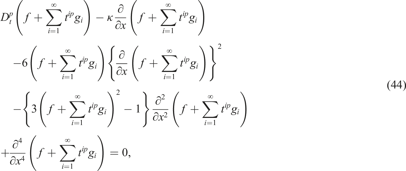
The following brief points outline Tantawy technique for analyzing problem (40):

Step (1) Substituting the subsequent Ansatz

$\mathbf{J}=f+\sum _{i=1}^{\infty }{t}^{ip}{g}_i,$

(43)

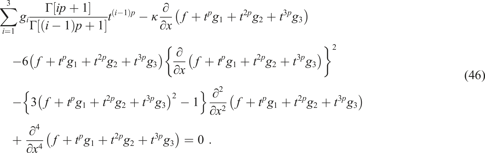
into equation (40) leads to

$\begin{array}{ll}\hfill & D_t^p\left(f+\sum _{i=1}^{\infty }{t}^{ip}{g}_i\right)-\kappa \frac{\partial }{\partial x}\left(f+\sum _{i=1}^{\infty }{t}^{ip}{g}_i\right)\hfill \\ \hfill & -6\left(f+\sum _{i=1}^{\infty }{t}^{ip}{g}_i\right){\left\{\frac{\partial }{\partial x}\left(f+\sum _{i=1}^{\infty }{t}^{ip}{g}_i\right)\right\}}^2\hfill \\ \hfill & -\left\{3{\left(f+\sum _{i=1}^{\infty }{t}^{ip}{g}_i\right)}^2-1\right\}\frac{{\partial }^2}{\partial x^2}\left(f+\sum _{i=1}^{\infty }{t}^{ip}{g}_i\right)\hfill \\ \hfill & +\frac{{\partial }^4}{\partial x^4}\left(f+\sum _{i=1}^{\infty }{t}^{ip}{g}_i\right)=0,\hfill \end{array}$

(44)

where $f\equiv f\left(x\right)$ represents the IC, $g_i\equiv g_i\left(x\right)$ denotes unknown functions of the variable x, which we aim to determine using the Tantawy technique and 0 < p ≤ 1.

• Step (2) According to solution (43), the fractional CDO $D_t^p\mathbf{J}$ can be written in the following manner

$D_t^p\mathbf{J}=\sum _{i=1}^{\infty }{g}_i{D}_t^p\left[t^{ip}\right]=\sum _{i=1}^{\infty }{g}_i\frac{\mathrm{\Gamma }\left[ip+1\right]}{\mathrm{\Gamma }\left[(i-1)p+1\right]}{t}^{(i-1)p}.$

(45)

• Step (3) For a certain number n ^th in the series solution (say n = 3) and by using equation (45) then equation (44) becomes

$\begin{array}{ll}\hfill & \sum _{i=1}^3{g}_i\frac{\mathrm{\Gamma }\left[ip+1\right]}{\mathrm{\Gamma }\left[(i-1)p+1\right]}{t}^{(i-1)p}-\kappa \frac{\partial }{\partial x}\left(f+t^p{g}_1+t^{2p}{g}_2+t^{3p}{g}_3\right)\hfill \\ \hfill & -6\left(f+t^p{g}_1+t^{2p}{g}_2+t^{3p}{g}_3\right){\left\{\frac{\partial }{\partial x}\left(f+t^p{g}_1+t^{2p}{g}_2+t^{3p}{g}_3\right)\right\}}^2\hfill \\ \hfill & -\left\{3{\left(f+t^p{g}_1+t^{2p}{g}_2+t^{3p}{g}_3\right)}^2-1\right\}\frac{{\partial }^2}{\partial x^2}\left(f+t^p{g}_1+t^{2p}{g}_2+t^{3p}{g}_3\right)\hfill \\ \hfill & +\frac{{\partial }^4}{\partial x^4}\left(f+t^p{g}_1+t^{2p}{g}_2+t^{3p}{g}_3\right)=0.\hfill \end{array}$

(46)

• Step (4) Now, by aggregating all terms associated with identical powers of t ^ip ∀ i = 0, 1, 2, 3, …, we obtain

$\sum _{i=0}{S}_i{t}^{ip}=S_0+S_1{t}^p+S_2{t}^{2p}+S_3{t}^{3p}+\cdots =0,$

(47)

with

$\begin{array}{ll}\hfill S_0& =\mathrm{\Gamma }\left[1+p\right]g_1-\kappa f^{\prime }-6f{\left(f^{\prime }\right)}^2+f^{\prime \prime }-3f^2{f}^{\prime \prime }+f^{\left(4\right)},\hfill \\ \hfill S_1& =\frac{\mathrm{\Gamma }\left[1+2p\right]g_2}{\mathrm{\Gamma }\left[1+p\right]}-6g_1{\left(f^{\prime }\right)}^2-\kappa f^{\prime }-12f{f}^{\prime }{g}_1^{\prime }-6f{f}^{\prime \prime }{g}_1+g_1^{\prime \prime }-3f^2{g}_1^{\prime \prime }+g_1^{\left(4\right)},\hfill \\ \hfill S_2& =\frac{\mathrm{\Gamma }\left[1+3p\right]g_3}{\mathrm{\Gamma }\left[1+2p\right]}-6g_2{\left(f^{\prime }\right)}^2-12g_1{g}_1^{\prime }{f}^{\prime }-6f{\left(g_1^{\prime }\right)}^2-\kappa g_2^{\prime }-12f{f}^{\prime }{g}_2^{\prime }-3f^{\prime \prime }{g}_1^2\hfill \\ \hfill & -6f{f}^{\prime \prime }{g}_2-6f{g}_1{g}_1^{\prime \prime }+g_2^{\prime \prime }-3f^2{g}_2^{\prime \prime }+g_2^{\left(4\right)},\hfill \\ \hfill & ⋮.\hfill \end{array}$

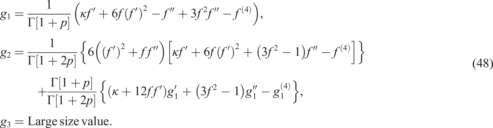
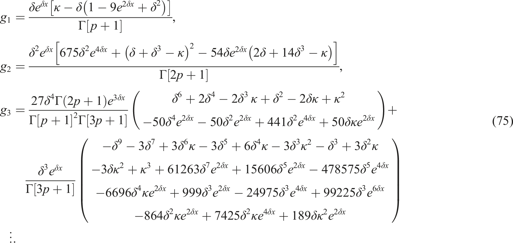
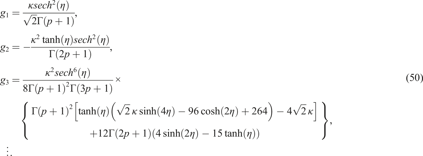
• Step (5) Now, we get the implicit values for g _i as functions of the IC f by setting the coefficients S _i ∀ i = 1, 2, 3,…to zero and then solving them for g₁, g₂, and g₃:

$\begin{array}{ll}\hfill g_1& =\frac{1}{\mathrm{\Gamma }\left[1+p\right]}\left(\kappa f^{\prime }+6f{\left(f^{\prime }\right)}^2-f^{\prime \prime }+3f^2{f}^{\prime \prime }-f^{\left(4\right)}\right),\hfill \\ \hfill g_2& =\frac{1}{\mathrm{\Gamma }\left[1+2p\right]}\left\{6\left({\left(f^{\prime }\right)}^2+f{f}^{\prime \prime }\right)\left[\kappa f^{\prime }+6f{\left(f^{\prime }\right)}^2+\left(3f^2-1\right)f^{\prime \prime }-f^{\left(4\right)}\right]\right\}\hfill \\ \hfill & +\frac{\mathrm{\Gamma }\left[1+p\right]}{\mathrm{\Gamma }\left[1+2p\right]}\left\{\left(\kappa +12f{f}^{\prime }\right)g_1^{\prime }+\left(3f^2-1\right)g_1^{\prime \prime }-g_1^{\left(4\right)}\right\},\hfill \\ \hfill g_3& =\text{Large\hspace{0.17em}size\hspace{0.17em}value}.\hfill \end{array}$

(48)

• Step (6) Inserting the value of the IC f

$f=\tanh \left[\eta \right],$

(49)

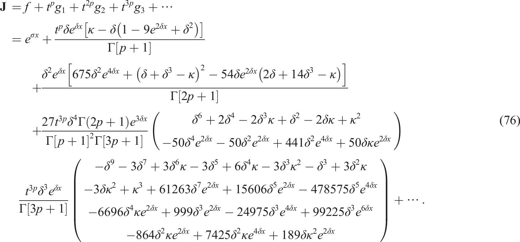
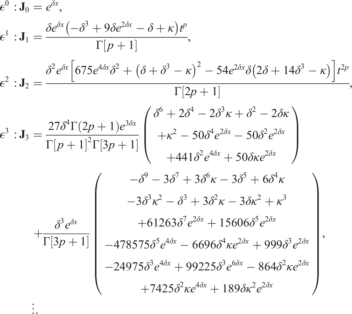
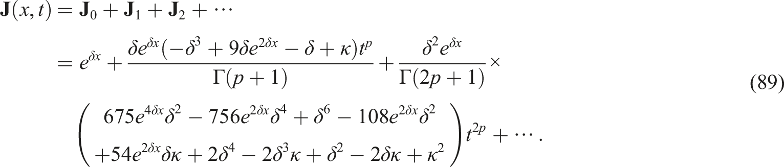
into the values of g₁, g₂, and g₃ given in equation (48), we get

$\begin{array}{ll}\hfill g_1& =\frac{\kappa {sech}^2\left(\eta \right)}{\sqrt{2}\mathrm{\Gamma }(p+1)},\hfill \\ \hfill g_2& =-\frac{{\kappa }^2\tanh \left(\eta \right){sech}^2\left(\eta \right)}{\mathrm{\Gamma }(2p+1)},\hfill \\ \hfill g_3& =\frac{{\kappa }^2{sech}^6\left(\eta \right)}{8\mathrm{\Gamma }{(p+1)}^2\mathrm{\Gamma }(3p+1)}\times \hfill \\ \hfill & \left\{\begin{array}{c}\hfill \mathrm{\Gamma }{(p+1)}^2\left[\tanh \left(\eta \right)\left(\sqrt{2}\kappa \sinh \left(4\eta \right)-96\cosh \left(2\eta \right)+264\right)-4\sqrt{2}\kappa \right]\hfill \\ \hfill +12\mathrm{\Gamma }(2p+1)\left(4\sinh \left(2\eta \right)-15\tanh \left(\eta \right)\right)\hfill \end{array}\right\},\hfill \\ \hfill ⋮& .\hfill \end{array}$

(50)

• Step (7) By substituting the obtained values of g₁, g₂, and g₃,… into Ansatz (43), we ultimately derive the approximate solution for problem (40) up to the third-order approximation as follows:

$\begin{array}{ll}\hfill \mathbf{J}& =f+t^p{g}_1+t^{2p}{g}_2+t^{3p}{g}_3+\cdots \hfill \\ \hfill & =\tanh \left[\eta \right]+\frac{t^p\kappa {sech}^2\left(\eta \right)}{\sqrt{2}\mathrm{\Gamma }(p+1)}-\frac{t^{2p}{\kappa }^2\tanh \left(\eta \right){sech}^2\left(\eta \right)}{\mathrm{\Gamma }(2p+1)}\hfill \\ \hfill & +\frac{t^{3p}{\kappa }^2{sech}^6\left(\eta \right)}{8\mathrm{\Gamma }{(p+1)}^2\mathrm{\Gamma }(3p+1)}\left\{\begin{array}{c}\hfill \mathrm{\Gamma }{(p+1)}^2\left[\begin{array}{c}\hfill \tanh \left(\eta \right)\left(\begin{array}{c}\hfill \sqrt{2}\kappa \sinh \left(4\eta \right)\hfill \\ \hfill -96\cosh \left(2\eta \right)+264\hfill \end{array}\right)\hfill \\ \hfill -4\sqrt{2}\kappa \hfill \end{array}\right]\hfill \\ \hfill +12\mathrm{\Gamma }(2p+1)\left(4\sinh \left(2\eta \right)-15\tanh \left(\eta \right)\right)\hfill \end{array}\right\}+\cdots .\hfill \end{array}$

(51)

Anatomy example (1) via the VITM

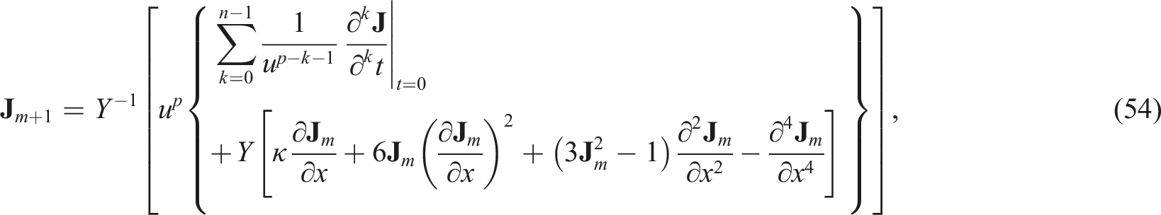
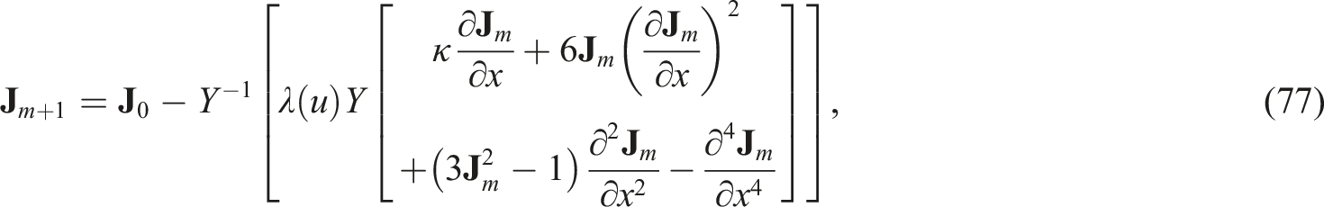
Here, we apply the VITM for analyzing equation (40). Accordingly, corrections functional for equation (40) can build as follows

$${\mathbf{J}}_{m+1}={\mathbf{J}}_m+Y^{-1}\left[\lambda \left(u\right)\left\{\begin{array}{l}{\frac{1}{u^p}Y\left[{\mathbf{J}}_{\mathbf{m}}\right]-{\displaystyle \sum }_{k=0}^{n-1}\frac{1}{u^{p-k-1}}\frac{{\partial }^k\mathbf{J}}{{\partial }^{k}t}|}_{t=0}\\ -Y\left[\kappa \frac{\partial {\mathbf{J}}_m}{\partial x}+6{\mathbf{J}}_m{\left(\frac{\partial {\mathbf{J}}_m}{\partial x}\right)}^2+\left(3{\mathbf{J}}_m^2-1\right)\frac{{\partial }^2{\mathbf{J}}_m}{{\partial x}^2}-\frac{{\partial }^4{\mathbf{J}}_m}{{\partial x}^4}\right]\end{array}\right\}\right],$$

(52)

with the following Lagrange multiplier λ(u):

$\lambda (u)=-u^p,$

(53)

where J_m+1 ≡ J_m+1(x, t) and J _m ≡ J _m (x, t).

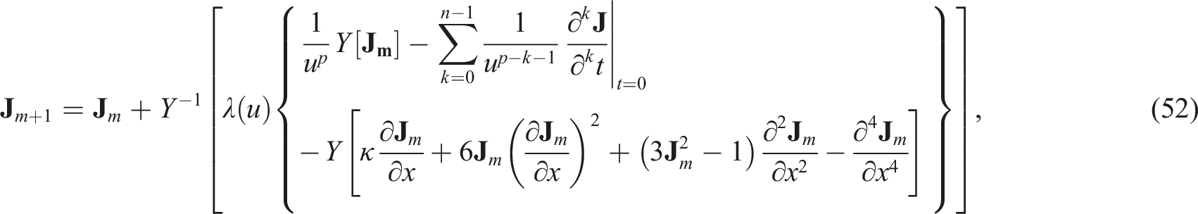
By inserting the value of λ(u) into equation (52), we get

$${\mathbf{J}}_{m+1}=Y^{-1}\left[u^p\left\{\begin{array}{l}{{\displaystyle \sum }_{k=0}^{n-1}\frac{1}{u^{p-k-1}}\frac{{\partial }^k\mathbf{J}}{{\partial }^{k}t}|}_{t=0}\\ +Y\left[\kappa \frac{\partial {\mathbf{J}}_m}{\partial x}+6{\mathbf{J}}_m{\left(\frac{\partial {\mathbf{J}}_m}{\partial x}\right)}^2+\left(3{\mathbf{J}}_m^2-1\right)\frac{{\partial }^2{\mathbf{J}}_m}{{\partial x}^2}-\frac{{\partial }^4{\mathbf{J}}_m}{{\partial x}^4}\right]\end{array}\right\}\right],$$

(54)

The zero-order approximation/IC reads

${\mathbf{J}}_0=\tanh \left(\eta \right).$

(55)

Now, for m = 0, the first-order approximation J₁ can be obtained by inserting the value of the zero-order approximation J₀(x, t) into equation (54) as follows

${\mathbf{J}}_1={\mathbf{J}}_0+Y^{-1}\left[u^p\left\{\kappa \frac{\partial {\mathbf{J}}_0}{\partial x}+6{\mathbf{J}}_0{\left(\frac{\partial {\mathbf{J}}_0}{\partial x}\right)}^2+\left(3{\mathbf{J}}_0^2-1\right)\frac{{\partial }^2{\mathbf{J}}_0}{\partial x^2}-\frac{{\partial }^4{\mathbf{J}}_0}{\partial x^4}\right\}\right],$

(56)

which leads to

${\mathbf{J}}_1=\tanh \left(\eta \right)+\frac{\kappa {sech}^2\left(\eta \right)t^p}{\sqrt{2}\mathrm{\Gamma }(p+1)}.$

(57)

Also, for m = 1, the second-order approximation J₂(x, t) can be obtained by inserting the value of the first-order approximation J₁ into equation (54) as follows

${\mathbf{J}}_2={\mathbf{J}}_0+Y^{-1}\left[u^p\left\{\kappa \frac{\partial {\mathbf{J}}_1}{\partial x}+6{\mathbf{J}}_1{\left(\frac{\partial {\mathbf{J}}_1}{\partial x}\right)}^2+\left(3{\mathbf{J}}_1^2-1\right)\frac{{\partial }^2{\mathbf{J}}_1}{\partial x^2}-\frac{{\partial }^4{\mathbf{J}}_1}{\partial x^4}\right\}\right],$

(58)

which leads to

$\begin{array}{ll}\hfill {\mathbf{J}}_2& =\tanh \left(\eta \right)+\frac{\kappa {sech}^2\left(\eta \right)t^p}{\sqrt{2}\mathrm{\Gamma }(p+1)}-\frac{{\kappa }^2\tanh \left(\eta \right){sech}^2\left(\eta \right)t^{2p}}{\sqrt{2}\mathrm{\Gamma }(2p+1)}\hfill \\ \hfill & +\frac{3{\kappa }^2\mathrm{\Gamma }(2p+1)(4\cosh (2\eta )-11)\tanh \left(\eta \right){sech}^6\left(\eta \right)t^{3p}}{2\mathrm{\Gamma }{(p+1)}^2\mathrm{\Gamma }(3p+1)}\hfill \\ \hfill & +\frac{3{\kappa }^3\mathrm{\Gamma }(3p+1)(3\cosh (2\eta )-4){sech}^8\left(\eta \right)t^{4p}}{2\sqrt{2}\mathrm{\Gamma }{(p+1)}^3\mathrm{\Gamma }(4p+1)}.\hfill \end{array}$

(59)

We finally get the analytical approximation to equation (40) until the second-order as follows

$\begin{array}{ll}\hfill \mathbf{J}& =\tanh \left(\eta \right)+\frac{\kappa {sech}^2\left(\eta \right)t^p}{\sqrt{2}\mathrm{\Gamma }(p+1)}-\frac{{\kappa }^2\tanh \left(\eta \right){sech}^2\left(\eta \right)t^{2p}}{\sqrt{2}\mathrm{\Gamma }(2p+1)}\hfill \\ \hfill & +\frac{3{\kappa }^2\mathrm{\Gamma }(2p+1)(4\cosh (2\eta )-11)\tanh \left(\eta \right){sech}^6\left(\eta \right)t^{3}p}{2\mathrm{\Gamma }{(p+1)}^2\mathrm{\Gamma }(3p+1)}\hfill \\ \hfill & +\frac{3{\kappa }^3\mathrm{\Gamma }(3p+1)(3\cosh (2\eta )-4){sech}^8\left(\eta \right)t^{4p}}{2\sqrt{2}\mathrm{\Gamma }{(p+1)}^3\mathrm{\Gamma }(4p+1)}+\cdots .\hfill \end{array}$

(60)

Anatomy example (1) via the HPTM

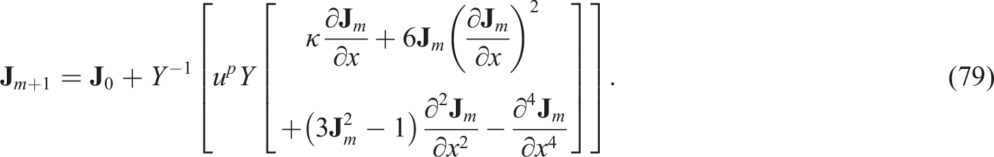
Here, the HPTM is applied for analyzing problem (40). First, we apply the YT on equation (40)

$Y\left[D_t^p\mathbf{J}\right]=Y\left[\kappa \frac{\partial \mathbf{J}}{\partial x}+6\mathbf{J}{\left(\frac{\partial \mathbf{J}}{\partial x}\right)}^2+\left(3{\mathbf{J}}^2-1\right)\frac{{\partial }^2\mathbf{J}}{\partial x^2}-\frac{{\partial }^4\mathbf{J}}{\partial x^4}\right],$

(61)

which leads to

$\frac{1}{u^p}\{\mathcal{R}(u)-u\mathbf{J}(0)\}=Y\left[\kappa \frac{\partial \mathbf{J}}{\partial x}+6\mathbf{J}{\left(\frac{\partial \mathbf{J}}{\partial x}\right)}^2+\left(3{\mathbf{J}}^2-1\right)\frac{{\partial }^2\mathbf{J}}{\partial x^2}-\frac{{\partial }^4\mathbf{J}}{\partial x^4}\right],$

(62)

and then we get

$\mathcal{R}(u)=u\mathbf{J}(0)+u^p\left[\kappa \frac{\partial \mathbf{J}}{\partial x}+6\mathbf{J}{\left(\frac{\partial \mathbf{J}}{\partial x}\right)}^2+\left(3{\mathbf{J}}^2-1\right)\frac{{\partial }^2\mathbf{J}}{\partial x^2}-\frac{{\partial }^4\mathbf{J}}{\partial x^4}\right].$

(63)

Now, by applying inverse YT on equation (63), we have

$\begin{array}{ll}\hfill \mathbf{J}& =\mathbf{J}(0)+Y^{-1}\left[u^p\left\{Y\left[\kappa \frac{\partial \mathbf{J}}{\partial x}+6\mathbf{J}{\left(\frac{\partial \mathbf{J}}{\partial x}\right)}^2+\left(3{\mathbf{J}}^2-1\right)\frac{{\partial }^2\mathbf{J}}{\partial x^2}-\frac{{\partial }^4\mathbf{J}}{\partial x^4}\right]\right\}\right]\hfill \\ \hfill & =\tanh \left(\eta \right)+Y^{-1}\left[u^p\left\{Y\left[\kappa \frac{\partial \mathbf{J}}{\partial x}+6\mathbf{J}{\left(\frac{\partial \mathbf{J}}{\partial x}\right)}^2+\left(3{\mathbf{J}}^2-1\right)\frac{{\partial }^2\mathbf{J}}{\partial x^2}-\frac{{\partial }^4\mathbf{J}}{\partial x^4}\right]\right\}\right].\hfill \end{array}$

(64)

According to the HPM, we have

$\begin{array}{ll}\hfill \sum _{k=0}^{\infty }{ϵ}^k{\mathbf{J}}_k& =\tanh \left(\eta \right)+ϵ\left\{Y^{-1}\left[u^{p}Y\left[\kappa \frac{\partial }{\partial x}\left(\sum _{k=0}^{\infty }{ϵ}^k{\mathbf{J}}_k\right)+6\left(\sum _{k=0}^{\infty }{ϵ}^k{H}_k\right)\right.\right.\right.\hfill \\ \hfill & \left.\left.\left.+3\left(\sum _{k=0}^{\infty }{ϵ}^k{H}_k\right)-\frac{{\partial }^2}{\partial x^2}\left(\sum _{k=0}^{\infty }{ϵ}^k{\mathbf{J}}_k\right)-\frac{{\partial }^4}{\partial x^4}\left(\sum _{k=0}^{\infty }{ϵ}^k{\mathbf{J}}_k\right)\right]\right]\right\},\hfill \end{array}$

where J _k ≡ J _k (x, t) and H _k ≡ H _k (x, t) ∀ k = 0, 1, 2, 3, ⋯ .

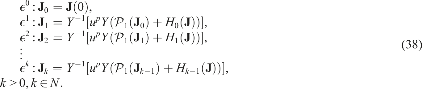
Collecting the coefficients of ϵ and solving them, the following recurrence values are obtained

$\begin{array}{ll}\hfill {ϵ}^0& :{\mathbf{J}}_0=\tanh \left[\eta \right],\hfill \\ \hfill {ϵ}^1& :{\mathbf{J}}_1=\frac{\kappa {sech}^2\left[\eta \right]t^p}{\sqrt{2}\mathrm{\Gamma }(p+1)},\hfill \\ \hfill {ϵ}^2& :{\mathbf{J}}_2=-\frac{{\kappa }^2\sinh \left[\eta \right]t^{2p}}{{\cosh }^3\left[\eta \right]\mathrm{\Gamma }(2p+1)},\hfill \\ \hfill {ϵ}^3& :{\mathbf{J}}_3=\frac{t^{3p}{\kappa }^2{sech}^6\left(\eta \right)}{8\mathrm{\Gamma }{(p+1)}^2\mathrm{\Gamma }(3p+1)}\times \hfill \\ \hfill & \left\{\begin{array}{c}\hfill \mathrm{\Gamma }{(p+1)}^2\left[\tanh \left(\eta \right)\left(\sqrt{2}\kappa \sinh \left(4\eta \right)-96\cosh \left(2\eta \right)+264\right)-4\sqrt{2}\kappa \right]\hfill \\ \hfill +12\mathrm{\Gamma }(2p+1)\left(4\sinh \left(2\eta \right)-15\tanh \left(\eta \right)\right)\hfill \end{array}\right\},\hfill \\ \hfill & ⋮.\hfill \end{array}$

Thus, the approximate solution according to the HPTM can be written in the following series form

$\begin{array}{l}\mathbf{J}={\mathbf{J}}_0+{\mathbf{J}}_1+{\mathbf{J}}_2+{\mathbf{J}}_3+\cdots \hfill \\ =\tanh \left[\eta \right]+\frac{\kappa {sech}^2\left[\eta \right]t^p}{\sqrt{2}\mathrm{\Gamma }(p+1)}-\frac{{\kappa }^2\sinh \left[\eta \right]t^{2p}}{{\cosh }^3\left[\eta \right]\mathrm{\Gamma }(2p+1)}+\frac{t^{3p}{\kappa }^2{sech}^6\left(\eta \right)}{8\mathrm{\Gamma }{(p+1)}^2\mathrm{\Gamma }(3p+1)}\times \hfill \\ \left\{\begin{array}{c}\hfill \mathrm{\Gamma }{(p+1)}^2\left[\tanh \left(\eta \right)\left(\sqrt{2}\kappa \sinh \left(4\eta x\right)-96\cosh \left(2\eta \right)+264\right)-4\sqrt{2}\kappa \right]\hfill \\ \hfill +12\mathrm{\Gamma }(2p+1)\left(4\sinh \left(2\eta \right)-15\tanh \left(\eta \right)\right)\hfill \end{array}\right\}+\cdots .\hfill \end{array}$

(65)

The approximations (51) and (65) show that both approximations are exactly the same, indicating that the Tantawy Technique yields the same approximations as HPTM. Consequently, we shall focus exclusively on one of these approximations in our numerical analysis. However, the Tantawy Technique is distinguished by its straightforward application, requiring no intricate computations and yielding higher order approximations promptly, in contrast to HPTM, which necessitates some time to achieve these approximations.

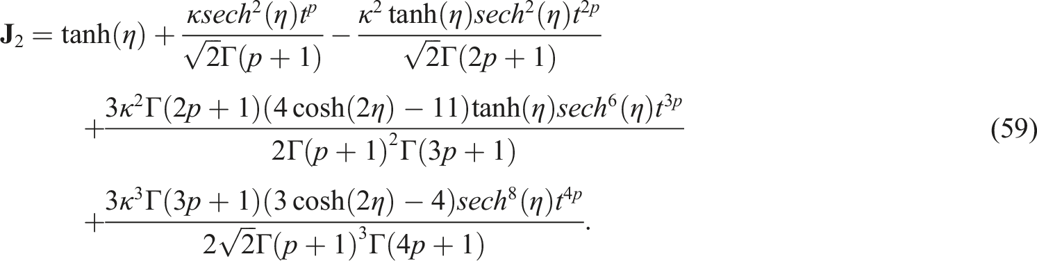
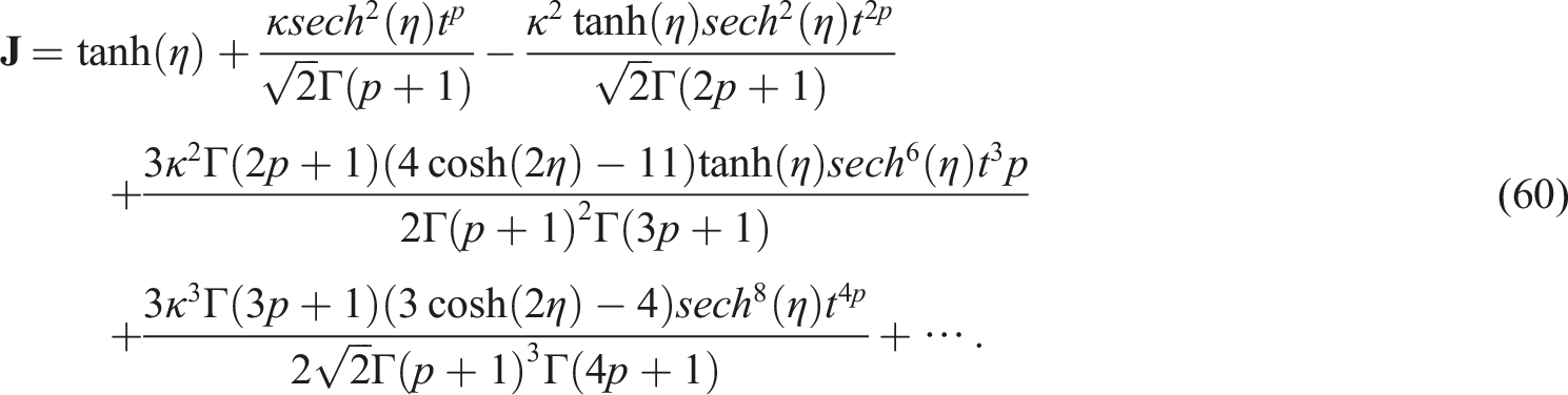
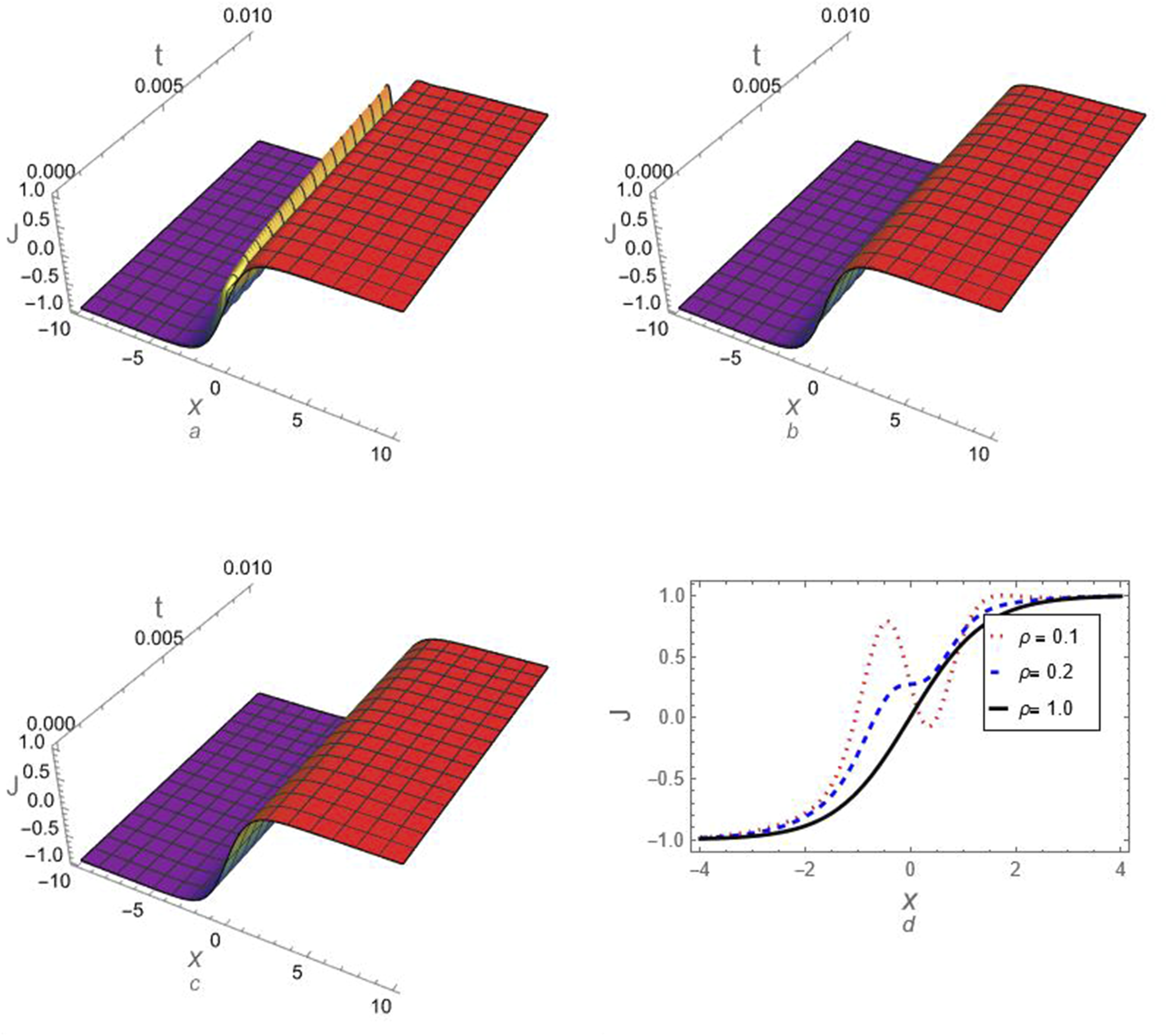
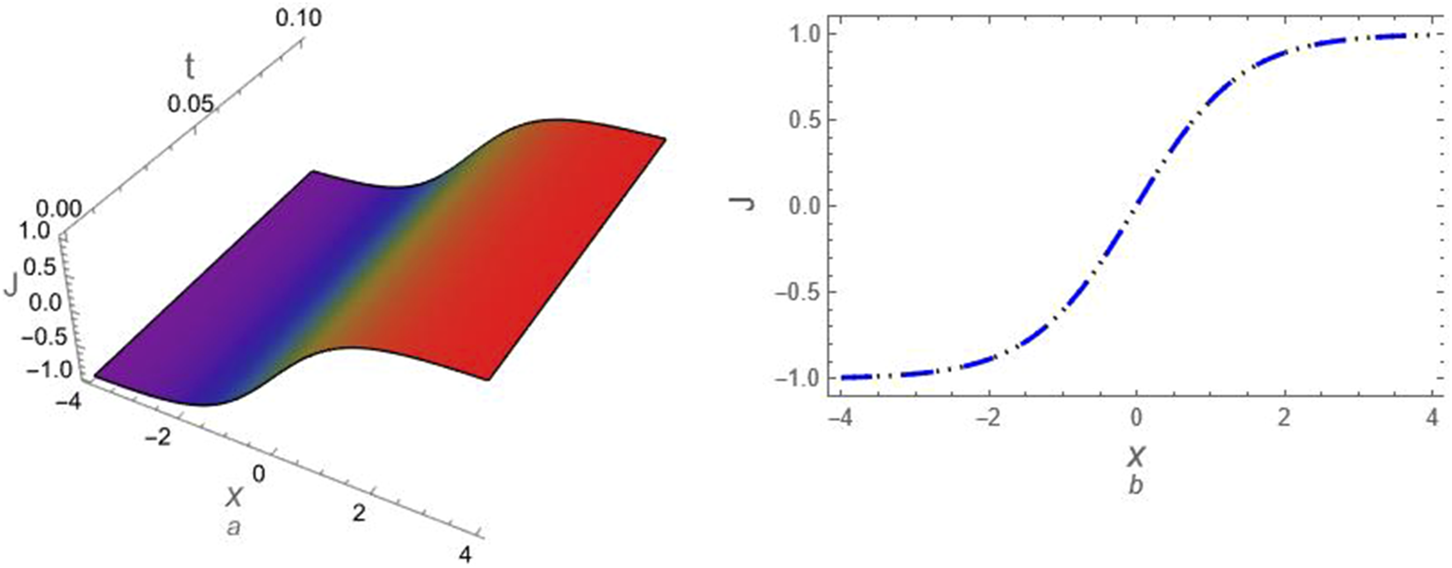
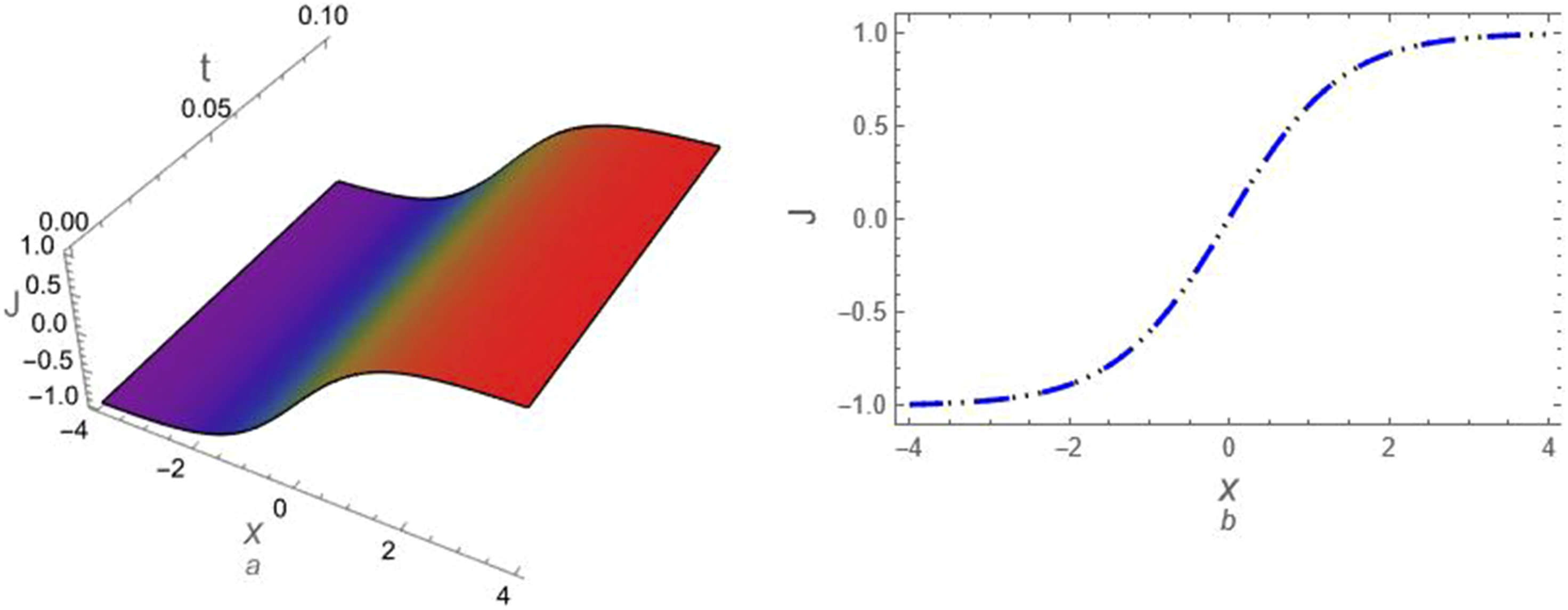
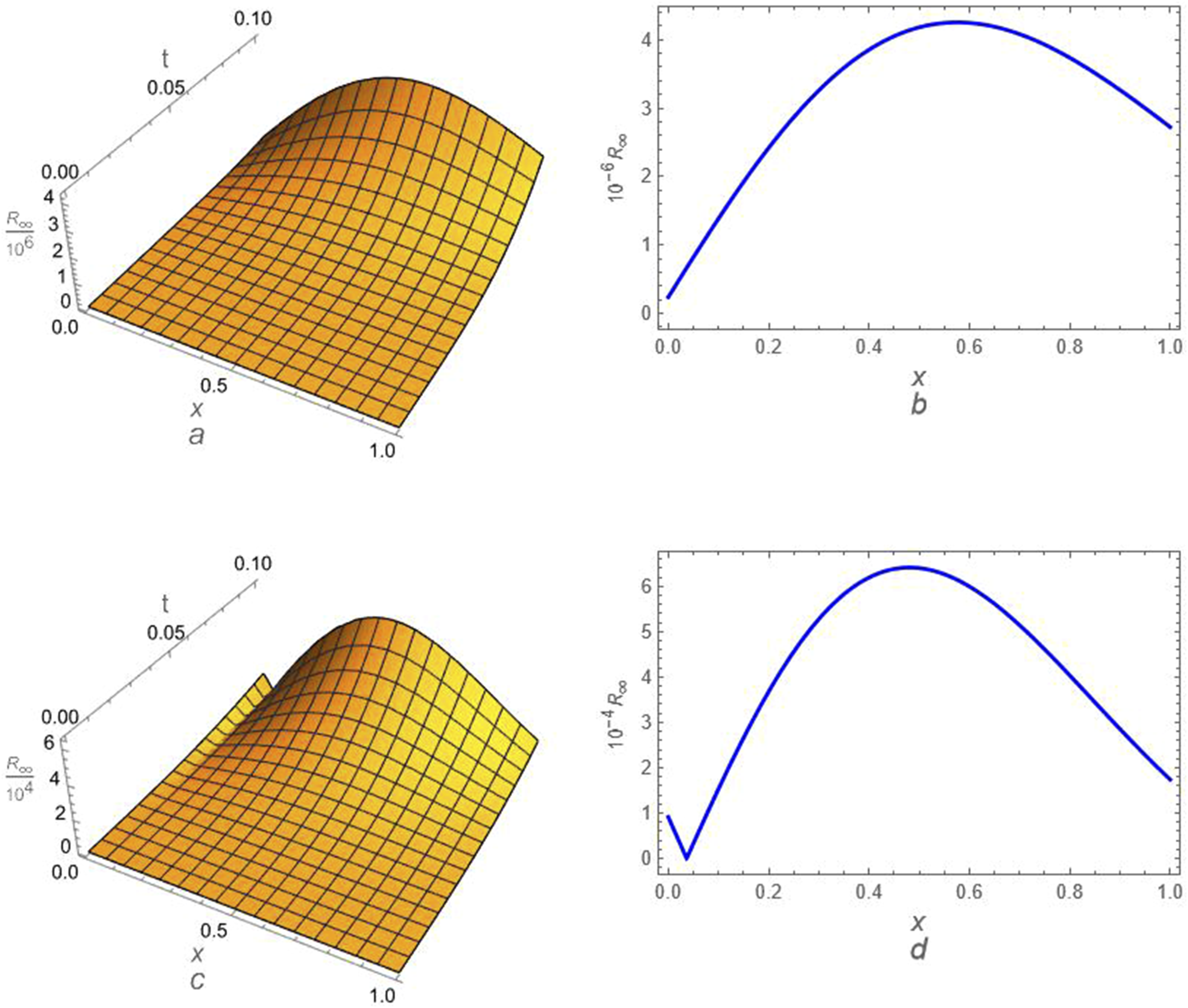
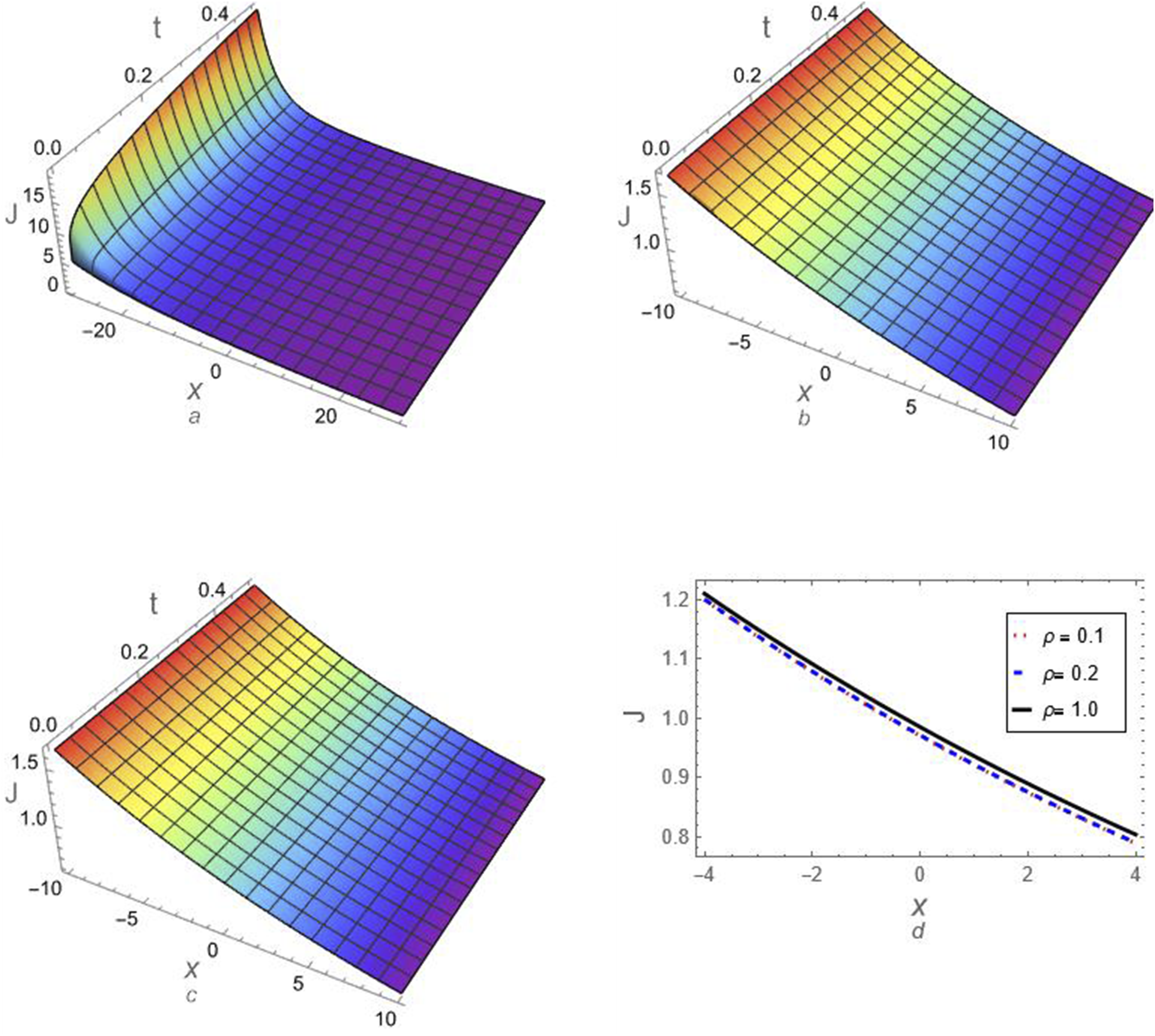
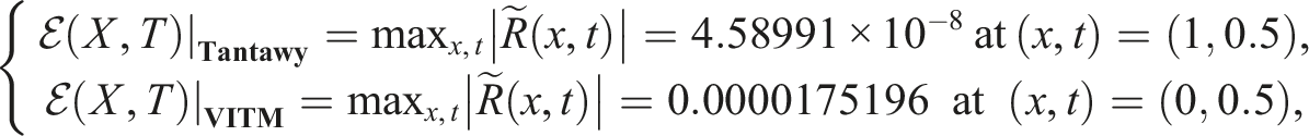
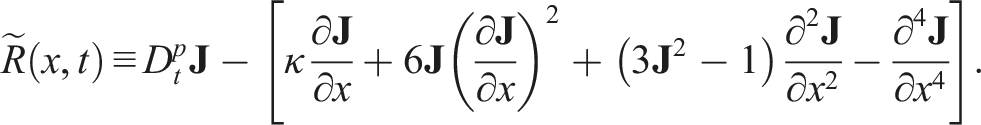
The derived approximation (51) and (60) using the Tantawy Technique/HPTM and VITM to equation (40) are, respectively, numerically examined against the fractional-order parameter “p” as elucidated in Figures 1 and 2. Note here that Additionally, the fractional-order solution shows that when the value of p approaches the integer-order, the solution approaches the exact solution. In Figures 3 and 4, we also graphically compared the approximation (51) using the Tantawy Technique and the approximation (60) using VITM with the exact solution (42) of equation (40) for the integer case to verify the effectiveness and stability of the used methods, especially the Tantawy Technique and the HPTM. Figures 3 and 4 demonstrate the total agreement between the analytical approximations (51) and (60) with the exact solution (42), confirming the high accuracy of the obtained approximations, especially the approximations (51) and (65) that have derived using the Tantawy Technique and the HPTM. Furthermore, Figure 5 shows the absolute error for all derived approximations (51) and (60) as compared to the exact solution (42). Figure 5 displays the absolute error of all approximations using the Tantawy Technique and VITM. The comparative investigation demonstrated that the Tantawy Technique showed markedly superior accuracy compared to the VITM. These findings validate the accuracy of the employed schemes, especially the Tantawy Technique/HPTM. As a result, our results’ physical interpretation could be a helpful tool for examining additional research on nonlinear wave phenomena in scientific domains.

Figure 1.

The analytical approximation (51) to equation (40) using the Tantawy Technique is plotted against the fractional-order parameter p: (a) 3D-graph for p = .1, (b) 3D-graph for p = .2, (c) 3D-graph for p = 1, and (d) 2D-graph for different values of p.

Figure 2.

The analytical approximation (60) to equation (40) using the VITM is plotted against the fractional-order parameter p: (a) 3D-graph for p = .1, (b) 3D-graph for p = .2, (c) 3D-graph for p = 1, and (d) 2D-graph for different values of p.

Figure 3.

The comparison between the approximation (51) using the Tantawy Technique at p = 1 and the exact solution (42): (a) 3D-graph in the $\left(x,t\right)-$ plane and (b) 2D-graph at t = 0.1.

Figure 4.

The comparison between the approximation (60) using the VITM at p = 1 and the exact solution (42): (a) 3D-graph in the $\left(x,t\right)-$ plane and (b) 2D-graph at t = 0.1.

Figure 5.

The comparison between the absolute error R _∞ of the approximations (51) and (60) for p = 1: (a) 3D-graph for R _∞ to the approximation (51) in the 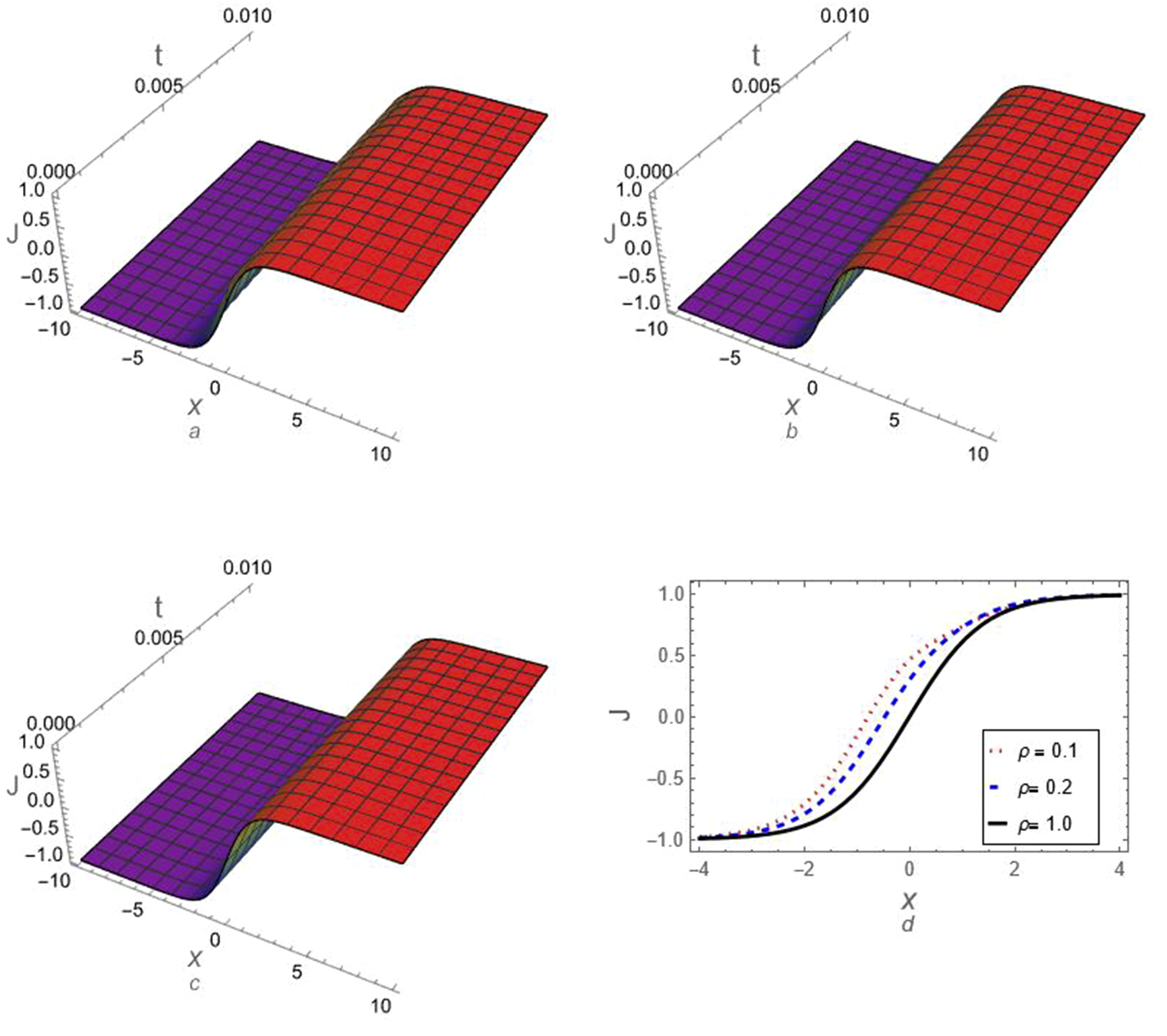$\left(x,t\right)-$ plane and (b) 2D-graph at t = 0.1 to the approximation (51), (c) 3D-graph for R _∞ to the approximation (60) in the $\left(x,t\right)-$ plane and (d) 2D-graph at t = 0.1 to the approximation (60).

Example (2)

Here, we consider the same example (1) but with a new IC as follows ⁴²

$D_t^p\mathbf{J}=\kappa \frac{\partial \mathbf{J}}{\partial x}+6\mathbf{J}{\left(\frac{\partial \mathbf{J}}{\partial x}\right)}^2+\left(3{\mathbf{J}}^2-1\right)\frac{{\partial }^2\mathbf{J}}{\partial x^2}-\frac{{\partial }^4\mathbf{J}}{\partial x^4},$

(66)

with

${\mathbf{J}(x,0)\equiv \mathbf{J}}_0=e^{\delta x},$

(67)

where $\mathbf{J}\equiv \mathbf{J}\left(x,t\right)$ and $0<p\le 1$ .

This problem will also be analyzed using the Tantawy Technique, the VITM, and the HPTM.

Anatomy example (2) via the Tantawy technique

The following brief points outline Tantawy technique for analyzing problem (66):

Step (1) By inserting the subsequent Ansatz

$\mathbf{J}=f+\sum _{i=1}^{\infty }{t}^{ip}{g}_i,$

(68)

into equation (66), we get

$\begin{array}{ll}\hfill & D_t^p\left(f+\sum _{i=1}^{\infty }{t}^{ip}{g}_i\right)-\kappa \frac{\partial }{\partial x}\left(f+\sum _{i=1}^{\infty }{t}^{ip}{g}_i\right)\hfill \\ \hfill & -6\left(f+\sum _{i=1}^{\infty }{t}^{ip}{g}_i\right){\left\{\frac{\partial }{\partial x}\left(f+\sum _{i=1}^{\infty }{t}^{ip}{g}_i\right)\right\}}^2\hfill \\ \hfill & -\left\{3{\left(f+\sum _{i=1}^{\infty }{t}^{ip}{g}_i\right)}^2-1\right\}\frac{{\partial }^2}{\partial x^2}\left(f+\sum _{i=1}^{\infty }{t}^{ip}{g}_i\right)\hfill \\ \hfill & +\frac{{\partial }^4}{\partial x^4}\left(f+\sum _{i=1}^{\infty }{t}^{ip}{g}_i\right)=0,\hfill \end{array}$

(69)

where $f\equiv f\left(x\right)$ represents the IC, $g_i\equiv g_i\left(x\right)$ denotes unknown functions of the variable x, which we aim to determine using the Tantawy technique and 0 < p ≤ 1.

• Step (2) According to solution (68), the fractional CDO $D_t^p\mathbf{J}$ can be written in the following manner

$D_t^p\mathbf{J}=\sum _{i=1}^{\infty }{g}_i{D}_t^p\left[t^{ip}\right]=\sum _{i=1}^{\infty }{g}_i\frac{\mathrm{\Gamma }\left[ip+1\right]}{\mathrm{\Gamma }\left[(ip-1)p+1\right]}{t}^{(i-1)p}.$

(70)

• Step (3) For a certain number n ^th in the series solution (say n = 3) and by using equation (70) then equation (44) becomes

$\begin{array}{ll}\hfill & \sum _{i=1}^3{g}_i\frac{\mathrm{\Gamma }\left[ip+1\right]}{\mathrm{\Gamma }\left[(i-1)p+1\right]}{t}^{(i-1)p}-\kappa \frac{\partial }{\partial x}\left(f+t^p{g}_1+t^{2p}{g}_2+t^{3p}{g}_3\right)\hfill \\ \hfill & -6\left(f+t^p{g}_1+t^{2p}{g}_2+t^{3p}{g}_3\right){\left\{\frac{\partial }{\partial x}\left(f+t^p{g}_1+t^{2p}{g}_2+t^{3p}{g}_3\right)\right\}}^2\hfill \\ \hfill & -\left\{3{\left(f+t^p{g}_1+t^{2p}{g}_2+t^{3p}{g}_3\right)}^2-1\right\}\frac{{\partial }^2}{\partial x^2}\left(f+t^p{g}_1+t^{2p}{g}_2+t^{3p}{g}_3\right)\hfill \\ \hfill & \hspace{1em}+\frac{{\partial }^4}{\partial x^4}\left(f+t^p{g}_1+t^{2p}{g}_2+t^{3p}{g}_3\right)=0.\hfill \end{array}$

(71)

• Step (4) Now, by aggregating all terms associated with identical powers of t ^ip ∀ i = 0, 1, 2, 3, …, we obtain

$\sum _{j=0}{S}_j{t}^{jp}=S_0+S_1{t}^p+S_2{t}^{2p}+S_3{t}^{3p}+\cdots =0,$

(72)

with

$\begin{array}{ll}\hfill S_0& =\mathrm{\Gamma }\left[1+p\right]g_1-\kappa f^{\prime }-6f{\left(f^{\prime }\right)}^2+f^{\prime \prime }-3f^2{f}^{\prime \prime }+f^{\left(4\right)},\hfill \\ \hfill S_1& =\frac{\mathrm{\Gamma }\left[1+2p\right]g_2}{\mathrm{\Gamma }\left[1+p\right]}-6g_1{\left(f^{\prime }\right)}^2-\kappa f^{\prime }-12f{f}^{\prime }{g}_1^{\prime }-6f{f}^{\prime \prime }{g}_1+g_1^{\prime \prime }-3f^2{g}_1^{\prime \prime }+g_1^{\left(4\right)},\hfill \\ \hfill S_2& =\frac{\mathrm{\Gamma }\left[1+3p\right]g_3}{\mathrm{\Gamma }\left[1+2p\right]}-6g_2{\left(f^{\prime }\right)}^2-12g_1{g}_1^{\prime }{f}^{\prime }-6f{\left(g_1^{\prime }\right)}^2-\kappa g_2^{\prime }-12f{f}^{\prime }{g}_2^{\prime }-3f^{\prime \prime }{g}_1^2\hfill \\ \hfill & -6f{f}^{\prime \prime }{g}_2-6f{g}_1{g}_1^{\prime \prime }+g_2^{\prime \prime }-3f^2{g}_2^{\prime \prime }+g_2^{\left(4\right)},\hfill \\ \hfill & ⋮.\hfill \end{array}$

• Step (5) The implicit values for g _i as functions of the IC f can be obtained by setting the coefficients S _i ∀ i = 1, 2, 3,…to zero and then solving them for g₁, g₂, and g which leads to

$\begin{array}{ll}\hfill g_1& =\frac{1}{\mathrm{\Gamma }\left[1+p\right]}\left(\kappa f^{\prime }+6f{\left(f^{\prime }\right)}^2-f^{\prime \prime }+3f^2{f}^{\prime \prime }-f^{\left(4\right)}\right),\hfill \\ \hfill g_2& =\frac{1}{\mathrm{\Gamma }\left[1+2p\right]}\left\{6\left({\left(f^{\prime }\right)}^2+f{f}^{\prime \prime }\right)\left[\kappa f^{\prime }+6f{\left(f^{\prime }\right)}^2+\left(3f^2-1\right)f^{\prime \prime }-f^{\left(4\right)}\right]\right\}\hfill \\ \hfill & +\frac{\mathrm{\Gamma }\left[1+p\right]}{\mathrm{\Gamma }\left[1+2p\right]}\left\{\left(\kappa +12f{f}^{\prime }\right)g_1^{\prime }+\left(3f^2-1\right)g_1^{\prime \prime }-g_1^{\left(4\right)}\right\}\hfill \\ \hfill g_3& =\text{Large\hspace{0.17em}size\hspace{0.17em}value}.\hfill \end{array}$

(73)

• Step (6) Inserting the value of the IC f

$f=e^{\sigma x},$

(74)

into the values of g₁, g₂, and g₃ given in equation (73), we get

$\begin{array}{ll}\hfill g_1& =\frac{\delta e^{\delta x}\left[\kappa -\delta \left(1-9e^{2\delta x}+{\delta }^2\right)\right]}{\mathrm{\Gamma }\left[p+1\right]},\hfill \\ \hfill g_2& =\frac{{\delta }^2{e}^{\delta x}\left[675{\delta }^2{e}^{4\delta x}+{\left(\delta +{\delta }^3-\kappa \right)}^2-54\delta e^{2\delta x}\left(2\delta +14{\delta }^3-\kappa \right)\right]}{\mathrm{\Gamma }\left[2p+1\right]},\hfill \\ \hfill g_3& =\frac{27{\delta }^4\mathrm{\Gamma }(2p+1)e^{3\delta x}}{\mathrm{\Gamma }{\left[p+1\right]}^2\mathrm{\Gamma }\left[3p+1\right]}\left(\begin{array}{c}\hfill {\delta }^6+2{\delta }^4-2{\delta }^3\kappa +{\delta }^2-2\delta \kappa +{\kappa }^2\hfill \\ \hfill -50{\delta }^4{e}^{2\delta x}-50{\delta }^2{e}^{2\delta x}+441{\delta }^2{e}^{4\delta x}+50\delta \kappa e^{2\delta x}\hfill \end{array}\right)+\hfill \\ \hfill & \frac{{\delta }^3{e}^{\delta x}}{\mathrm{\Gamma }\left[3p+1\right]}\left(\begin{array}{c}\hfill -{\delta }^9-3{\delta }^7+3{\delta }^6\kappa -3{\delta }^5+6{\delta }^4\kappa -3{\delta }^3{\kappa }^2-{\delta }^3+3{\delta }^2\kappa \hfill \\ \hfill -3\delta {\kappa }^2+{\kappa }^3+61263{\delta }^7{e}^{2\delta x}+15606{\delta }^5{e}^{2\delta x}-478575{\delta }^5{e}^{4\delta x}\hfill \\ \hfill -6696{\delta }^4\kappa e^{2\delta x}+999{\delta }^3{e}^{2\delta x}-24975{\delta }^3{e}^{4\delta x}+99225{\delta }^3{e}^{6\delta x}\hfill \\ \hfill -864{\delta }^2\kappa e^{2\delta x}+7425{\delta }^2\kappa e^{4\delta x}+189\delta {\kappa }^2{e}^{2\delta x}\hfill \end{array}\right)\hfill \\ \hfill ⋮& .\hfill \end{array}$

(75)

• Step (7) By substituting the obtained values of g₁, g₂, and g₃,… into Ansatz (68), we ultimately derive the approximate solution for problem (40) up to the third-order approximation as follows:

$\begin{array}{ll}\hfill \mathbf{J}& =f+t^p{g}_1+t^{2p}{g}_2+t^{3p}{g}_3+\cdots \hfill \\ \hfill & =e^{\sigma x}+\frac{t^p\delta e^{\delta x}\left[\kappa -\delta \left(1-9e^{2\delta x}+{\delta }^2\right)\right]}{\mathrm{\Gamma }\left[p+1\right]}\hfill \\ \hfill & +\frac{{\delta }^2{e}^{\delta x}\left[675{\delta }^2{e}^{4\delta x}+{\left(\delta +{\delta }^3-\kappa \right)}^2-54\delta e^{2\delta x}\left(2\delta +14{\delta }^3-\kappa \right)\right]}{\mathrm{\Gamma }\left[2p+1\right]}\hfill \\ \hfill & +\frac{27t^{3p}{\delta }^4\mathrm{\Gamma }(2p+1)e^{3\delta x}}{\mathrm{\Gamma }{\left[p+1\right]}^2\mathrm{\Gamma }\left[3p+1\right]}\left(\begin{array}{c}\hfill {\delta }^6+2{\delta }^4-2{\delta }^3\kappa +{\delta }^2-2\delta \kappa +{\kappa }^2\hfill \\ \hfill -50{\delta }^4{e}^{2\delta x}-50{\delta }^2{e}^{2\delta x}+441{\delta }^2{e}^{4\delta x}+50\delta \kappa e^{2\delta x}\hfill \end{array}\right)\hfill \\ \hfill & \frac{t^{3p}{\delta }^3{e}^{\delta x}}{\mathrm{\Gamma }\left[3p+1\right]}\left(\begin{array}{c}\hfill -{\delta }^9-3{\delta }^7+3{\delta }^6\kappa -3{\delta }^5+6{\delta }^4\kappa -3{\delta }^3{\kappa }^2-{\delta }^3+3{\delta }^2\kappa \hfill \\ \hfill -3\delta {\kappa }^2+{\kappa }^3+61263{\delta }^7{e}^{2\delta x}+15606{\delta }^5{e}^{2\delta x}-478575{\delta }^5{e}^{4\delta x}\hfill \\ \hfill -6696{\delta }^4\kappa e^{2\delta x}+999{\delta }^3{e}^{2\delta x}-24975{\delta }^3{e}^{4\delta x}+99225{\delta }^3{e}^{6\delta x}\hfill \\ \hfill -864{\delta }^2\kappa e^{2\delta x}+7425{\delta }^2\kappa e^{4\delta x}+189\delta {\kappa }^2{e}^{2\delta x}\hfill \end{array}\right)+\cdots .\hfill \end{array}$

(76)

Anatomy example (2) via the VITM

According to the VITM, the corrections functional for equation (66) can be constructed as follows

${\mathbf{J}}_{m+1}={\mathbf{J}}_0-Y^{-1}\left[\lambda \left(u\right)Y\left[\begin{array}{c}\kappa \frac{\partial {\mathbf{J}}_m}{\partial x}+6{\mathbf{J}}_m{\left(\frac{\partial {\mathbf{J}}_m}{\partial x}\right)}^2\\ +\left(3{\mathbf{J}}_m^2-1\right)\frac{{\partial }^2{\mathbf{J}}_m}{\partial x^2}-\frac{{\partial }^4{\mathbf{J}}_m}{\partial x^4}\end{array}\right]\right],$

(77)

with the following Lagrange multiplier λ(u):

$\lambda (u)=-u^p,$

(78)

where J_m+1 ≡ J_m+1(x, t) and J _m ≡ J _m (x, t).

Substituting equation (78) into equation (77) implies

${\mathbf{J}}_{m+1}={\mathbf{J}}_0+Y^{-1}\left[u^{p}Y\left[\begin{array}{c}\kappa \frac{\partial {\mathbf{J}}_m}{\partial x}+6{\mathbf{J}}_m{\left(\frac{\partial {\mathbf{J}}_m}{\partial x}\right)}^2\\ +\left(3{\mathbf{J}}_m^2-1\right)\frac{{\partial }^2{\mathbf{J}}_m}{\partial x^2}-\frac{{\partial }^4{\mathbf{J}}_m}{\partial x^4}\end{array}\right]\right].$

(79)

The zeroth-order approximation reads

${\mathbf{J}}_0=e^{\delta x}.$

(80)

The first-order approximation J₁ can be estimated by inserting equation (80) into equation (79) for m = 0, as follows

${\mathbf{J}}_1={\mathbf{J}}_0+Y^{-1}\left[u^p\left\{\kappa \frac{\partial {\mathbf{J}}_0}{\partial x}+6{\mathbf{J}}_0{\left(\frac{\partial {\mathbf{J}}_0}{\partial x}\right)}^2+\left(3{\mathbf{J}}_0^2-1\right)\frac{{\partial }^2{\mathbf{J}}_0}{\partial x^2}-\frac{{\partial }^4{\mathbf{J}}_0}{\partial x^4}\right\}\right],$

(81)

which leads to

${\mathbf{J}}_1=e^{\delta x}+S_1{t}^p,$

(82)

with

$S_1=\frac{\delta e^{\delta x}(-{\delta }^3+9\delta e^{2\delta x}-\delta +\kappa )}{\mathrm{\Gamma }(p+1)}.$

Also, the second-order approximation J₂ can be obtained by inserting equation (82) into equation (79) for m = 1, as follows

${\mathbf{J}}_2={\mathbf{J}}_0+Y^{-1}\left[u^p\left\{\kappa \frac{\partial {\mathbf{J}}_1}{\partial x}+6{\mathbf{J}}_1{\left(\frac{\partial {\mathbf{J}}_1}{\partial x}\right)}^2+\left(3{\mathbf{J}}_1^2-1\right)\frac{{\partial }^2{\mathbf{J}}_1}{\partial x^2}-\frac{{\partial }^4{\mathbf{J}}_1}{\partial x^4}\right\}\right],$

(83)

which leads to

${\mathbf{J}}_2=e^{\delta }x+S_1{t}^p+S_2{t}^{2p}+S_3{t}^{3p}+S_4{t}^{4p},$

with

$\begin{array}{ll}\hfill S_2& =\frac{{\delta }^2{e}^{\delta x}\left[{\left({\delta }^3+\delta -\kappa \right)}^2-54\delta \left(14{\delta }^3+2\delta -\kappa \right)e^{2\delta x}+675{\delta }^2{e}^{4\delta x}\right]}{\mathrm{\Gamma }\left[2p+1\right]},\hfill \\ \hfill S_3& =\frac{27{\delta }^4\mathrm{\Gamma }\left[2p+1\right]e^{3\delta x}\left[{\left({\delta }^3+\delta -\kappa \right)}^2-50\delta \left({\delta }^3+\delta -\kappa \right)e^{2\delta x}+441{\delta }^2{e}^{4\delta x}\right]}{\mathrm{\Gamma }{\left[p+1\right]}^2\mathrm{\Gamma }\left[3p+1\right]},\hfill \\ \hfill S_4& =\frac{9{\delta }^5\mathrm{\Gamma }\left[3p+1\right]e^{3\delta x}\left(\kappa -{\delta }^3+9\delta e^{2\delta x}-\delta \right)}{\mathrm{\Gamma }{\left[p+1\right]}^3\mathrm{\Gamma }\left[4p+1\right]}\times \hfill \\ \hfill & \left[{\left({\delta }^3+\delta -\kappa \right)}^2-66\delta \left({\delta }^3+\delta -\kappa \right)e^{2\delta x}+729{\delta }^2{e}^{4\delta x}\right].\hfill \end{array}$

Finally, the analytical approximation to equation (66) until the second-order reads

$\mathbf{J}\left(x,t\right)=e^{\delta x}+S_1{t}^p+S_2{t}^{2p}+S_3{t}^{3p}+S_4{t}^{4p},$

(84)

where S _i ∀ i = 1, 2, 3, 4 are defined above.

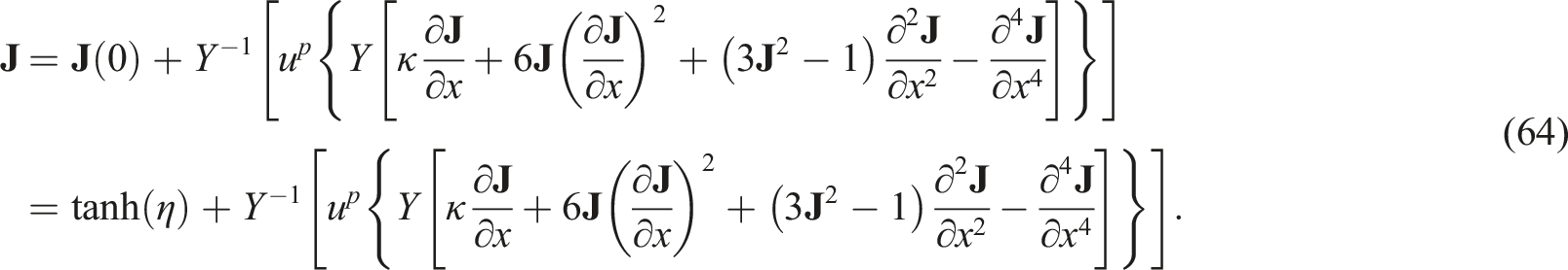
Anatomy example (2) via the HPTM

For analyzing problem (66) via HPTM, we first apply YT on equation (66)

$Y\left[D_t^p\mathbf{J}\right]=Y\left[\kappa \frac{\partial \mathbf{J}}{\partial x}+6\mathbf{J}{\left(\frac{\partial \mathbf{J}}{\partial x}\right)}^2+\left(3{\mathbf{J}}^2-1\right)\frac{{\partial }^2\mathbf{J}}{\partial x^2}-\frac{{\partial }^4\mathbf{J}}{\partial x^4}\right],$

(85)

which leads to

$\frac{1}{u^p}\{\mathcal{R}(u)-u\mathbf{J}(0)\}=Y\left[\kappa \frac{\partial \mathbf{J}}{\partial x}+6\mathbf{J}{\left(\frac{\partial \mathbf{J}}{\partial x}\right)}^2+\left(3{\mathbf{J}}^2-1\right)\frac{{\partial }^2\mathbf{J}}{\partial x^2}-\frac{{\partial }^4\mathbf{J}}{\partial x^4}\right],$

(86)

and then, we get

$\mathcal{R}(u)=u\mathbf{J}(0)+u^p\left[\kappa \frac{\partial \mathbf{J}}{\partial x}+6\mathbf{J}{\left(\frac{\partial \mathbf{J}}{\partial x}\right)}^2+\left(3{\mathbf{J}}^2-1\right)\frac{{\partial }^2\mathbf{J}}{\partial x^2}-\frac{{\partial }^4\mathbf{J}}{\partial x^4}\right].$

(87)

Applying the inverse YT on equation (87) yields

$\begin{array}{ll}\hfill \mathbf{J}& =\mathbf{J}(0)+Y^{-1}\left[u^p\left\{Y\left[\kappa \frac{\partial \mathbf{J}}{\partial x}+6\mathbf{J}{\left(\frac{\partial \mathbf{J}}{\partial x}\right)}^2+\left(3{\mathbf{J}}^2-1\right)\frac{{\partial }^2\mathbf{J}}{\partial x^2}-\frac{{\partial }^4\mathbf{J}}{\partial x^4}\right]\right\}\right],\hfill \\ \hfill & =e^{\delta x}+Y^{-1}\left[u^p\left\{Y\left[\kappa \frac{\partial \mathbf{J}}{\partial x}+6\mathbf{J}{\left(\frac{\partial \mathbf{J}}{\partial x}\right)}^2+\left(3{\mathbf{J}}^2-1\right)\frac{{\partial }^2\mathbf{J}}{\partial x^2}-\frac{{\partial }^4\mathbf{J}}{\partial x^4}\right]\right\}\right].\hfill \end{array}$

(88)

In terms of HPM, we get

$\begin{array}{ll}\hfill \sum _{k=0}^{\infty }{ϵ}^k{\mathbf{J}}_k& =e^{\delta x}+ϵ\left\{Y^{-1}\left[u^{p}Y\left[\kappa \frac{\partial }{\partial x}\left(\sum _{k=0}^{\infty }{ϵ}^k{\mathbf{J}}_k\right)+6\left(\sum _{k=0}^{\infty }{ϵ}^k{H}_k\right)\right.\right.\right.\hfill \\ \hfill & \left.\left.\left.+3\left(\sum _{k=0}^{\infty }{ϵ}^k{H}_k\right)-\frac{{\partial }^2}{\partial x^2}\left(\sum _{k=0}^{\infty }{ϵ}^k{\mathbf{J}}_k\right)-\frac{{\partial }^4}{\partial x^4}\left(\sum _{k=0}^{\infty }{ϵ}^k{\mathbf{J}}_k\right)\right]\right]\right\},\hfill \end{array}$

where J _k ≡ J _k (x, t) and H _k ≡ H _k (x, t) ∀ k = 0, 1, 2, 3, ⋯ .

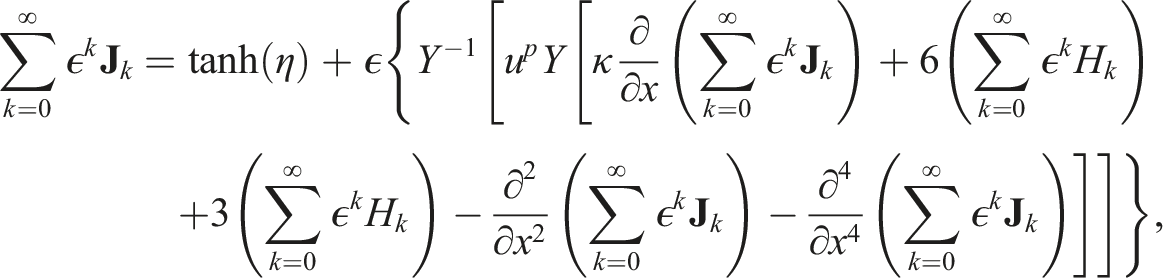
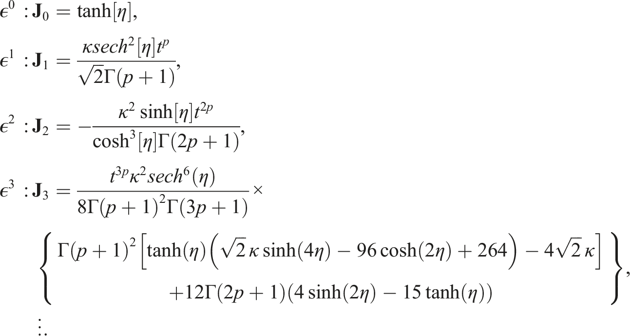
Collecting the coefficients of ϵ and solving them, the following recurrence values are obtained

$\begin{array}{ll}\hfill {ϵ}^0& :{\mathbf{J}}_0=e^{\delta x},\hfill \\ \hfill {ϵ}^1& :{\mathbf{J}}_1=\frac{\delta e^{\delta x}\left(-{\delta }^3+9\delta e^{2\delta x}-\delta +\kappa \right)t^p}{\mathrm{\Gamma }\left[p+1\right]},\hfill \\ \hfill {ϵ}^2& :{\mathbf{J}}_2=\frac{{\delta }^2{e}^{\delta x}\left[675e^{4\delta x}{\delta }^2+{\left(\delta +{\delta }^3-\kappa \right)}^2-54e^{2\delta x}\delta \left(2\delta +14{\delta }^3-\kappa \right)\right]t^{2p}}{\mathrm{\Gamma }\left[2p+1\right]},\hfill \\ \hfill {ϵ}^3& :{\mathbf{J}}_3=\frac{27{\delta }^4\mathrm{\Gamma }(2p+1)e^{3\delta x}}{\mathrm{\Gamma }{\left[p+1\right]}^2\mathrm{\Gamma }\left[3p+1\right]}\left(\begin{array}{c}\hfill {\delta }^6+2{\delta }^4-2{\delta }^3\kappa +{\delta }^2-2\delta \kappa \hfill \\ \hfill +{\kappa }^2-50{\delta }^4{e}^{2\delta x}-50{\delta }^2{e}^{2\delta x}\hfill \\ \hfill +441{\delta }^2{e}^{4\delta x}+50\delta \kappa e^{2\delta x}\hfill \end{array}\right)\hfill \\ \hfill & +\frac{{\delta }^3{e}^{\delta x}}{\mathrm{\Gamma }\left[3p+1\right]}\left(\begin{array}{c}\hfill -{\delta }^9-3{\delta }^7+3{\delta }^6\kappa -3{\delta }^5+6{\delta }^4\kappa \hfill \\ \hfill -3{\delta }^3{\kappa }^2-{\delta }^3+3{\delta }^2\kappa -3\delta {\kappa }^2+{\kappa }^3\hfill \\ \hfill +61263{\delta }^7{e}^{2\delta x}+15606{\delta }^5{e}^{2\delta x}\hfill \\ \hfill -478575{\delta }^5{e}^{4\delta x}-6696{\delta }^4\kappa e^{2\delta x}+999{\delta }^3{e}^{2\delta x}\hfill \\ \hfill -24975{\delta }^3{e}^{4\delta x}+99225{\delta }^3{e}^{6\delta x}-864{\delta }^2\kappa e^{2\delta x}\hfill \\ \hfill +7425{\delta }^2\kappa e^{4\delta x}+189\delta {\kappa }^2{e}^{2\delta x}\hfill \end{array}\right),\hfill \\ \hfill & ⋮.\hfill \end{array}$

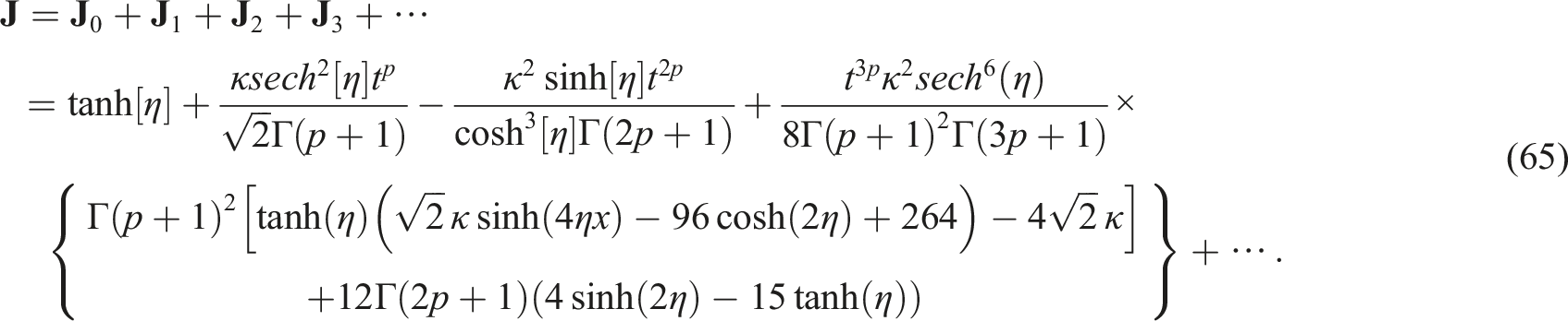
Thus, the approximate solution according to the HPTM can be written in the following series form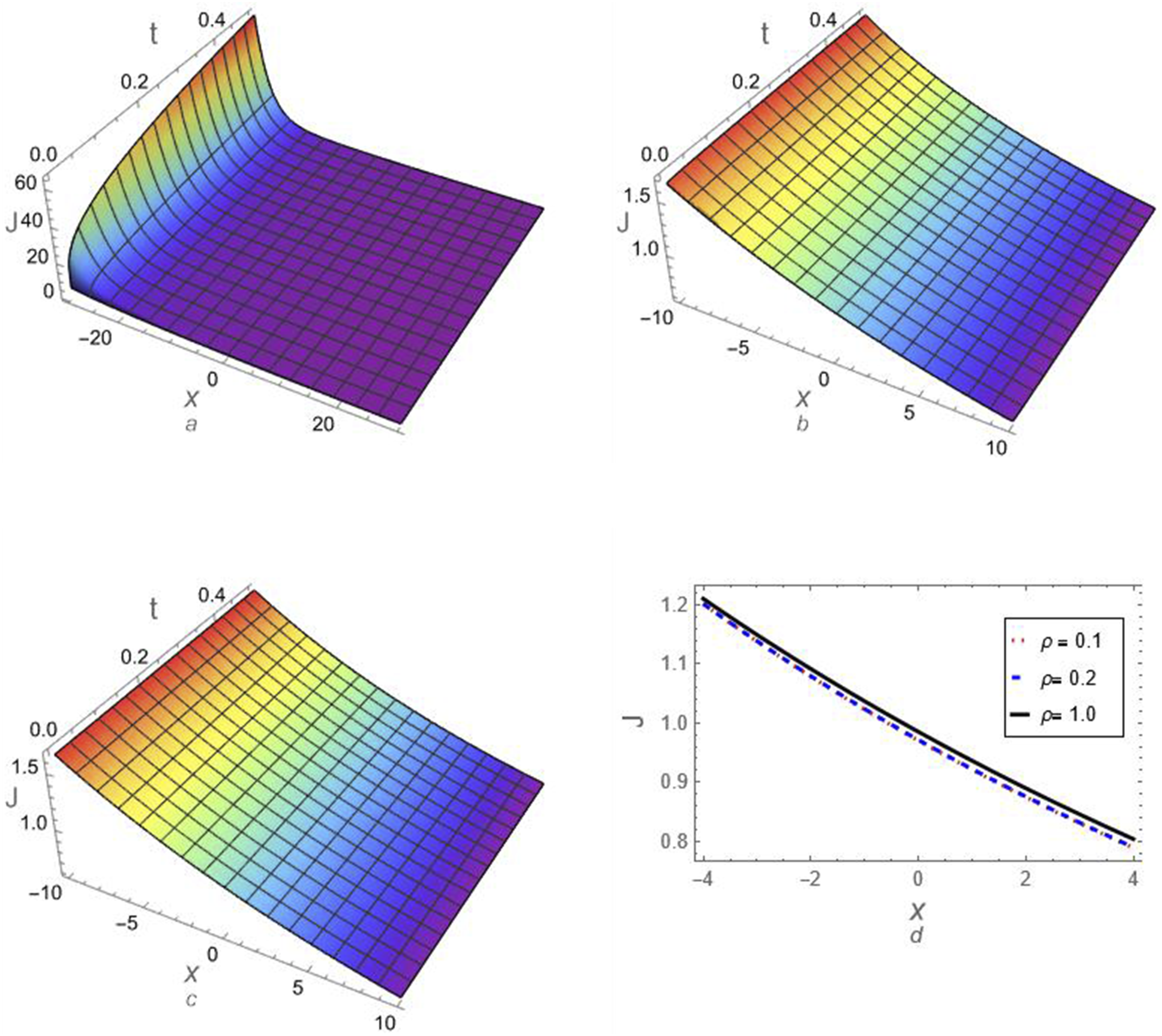

$\begin{array}{ll}\hfill \mathbf{J}\left(x,t\right)& ={\mathbf{J}}_0+{\mathbf{J}}_1+{\mathbf{J}}_2+\cdots \hfill \\ \hfill & =e^{\delta x}+\frac{\delta e^{\delta x}(-{\delta }^3+9\delta e^{2\delta x}-\delta +\kappa )t^p}{\mathrm{\Gamma }(p+1)}+\frac{{\delta }^2{e}^{\delta x}}{\mathrm{\Gamma }(2p+1)}\times \hfill \\ \hfill & \left(\begin{array}{c}\hfill 675e^{4\delta x}{\delta }^2-756e^{2\delta x}{\delta }^4+{\delta }^6-108e^{2\delta x}{\delta }^2\hfill \\ \hfill +54e^{2\delta x}\delta \kappa +2{\delta }^4-2{\delta }^3\kappa +{\delta }^2-2\delta \kappa +{\kappa }^2\hfill \end{array}\right)t^{2p}+\cdots .\hfill \end{array}$

(89)

The approximations (76) and (84) are investigated numerically, as evident in Figures 6 and 7. In these figures, we investigated the impact of the fractional-order parameter p on the behavior of the approximations (76) and (84). Also, it is clear that the two approximations (76) and (89) are identical, signifying that the Tantawy Technique produces the same approximations as HPTM. Due to the unavailability of the exact solution to problem (66), we estimated the maximum residual error $\mathcal{E}\left(x,t\right)$ for the approximations (76) and (84) in the study domain $\mathrm{\Omega }\forall x\in \left[\mathrm{0,1}\right]$ & $t\in \left[\mathrm{0,0.5}\right]$ , as follows:

$\left\{\begin{array}{c}\hfill {\left.\mathcal{E}\left(X,T\right)\right|}_{\mathbf{T}\mathbf{a}\mathbf{n}\mathbf{t}\mathbf{a}\mathbf{w}\mathbf{y}}={\max }_{x,t}\left|\tilde{R}(x,t)\right|=4.58991\times 10^{-8}\text{\hspace{0.17em}at\hspace{0.17em}}\left(x,t\right)=\left(\mathrm{1,0.5}\right),\hfill \\ \hfill {\left.\mathcal{E}\left(X,T\right)\right|}_{\mathbf{V}\mathbf{I}\mathbf{T}\mathbf{M}}={\max }_{x,t}\left|\tilde{R}(x,t)\right|=0.0000175196\text{\hspace{0.17em}at\hspace{0.17em}}\left(x,t\right)=\left(\mathrm{0,0.5}\right),\hfill \end{array}\right.$

with

$\tilde{R}(x,t)\equiv D_t^p\mathbf{J}-\left[\kappa \frac{\partial \mathbf{J}}{\partial x}+6\mathbf{J}{\left(\frac{\partial \mathbf{J}}{\partial x}\right)}^2+\left(3{\mathbf{J}}^2-1\right)\frac{{\partial }^2\mathbf{J}}{\partial x^2}-\frac{{\partial }^4\mathbf{J}}{\partial x^4}\right].$

It is clear that the approximation (76) using the Tantawy Technique is more accurate than the approximation (84) using The VIM. The obtained results demonstrate the high efficiency of the Tantawy technique in analyzing the most complicated and strong nonlinearity physical and engineering problems with high accuracy compared to other similar methods.

Figure 6.

The analytical approximation (76) to equation (66) using the Tantawy Technique is plotted against the fractional-order parameter p: (a) 3D-graph for p = .1, (b) 3D-graph for p = .2, (c) 3D-graph for p = 1, and (d) 2D-graph for different values of p.

Figure 7.

The analytical approximation (84) to equation (40) using the VITM is plotted against the fractional-order parameter p: (a) 3D-graph for p = .1, (b) 3D-graph for p = .2, (c) 3D-graph for p = 1, and (d) 2D-graph for different values of p.

Conclusion

In conclusion, we have examined the iterative approaches to building highly accurate analytical approximations with various initial conditions for the fourth-order time-fractional nonlinear Cahn–Hilliard equations. For this purpose, the Tantawy Technique has been introduced for the first time for analyzing different types of differential equations. Given that the Tantawy Technique is a novel technique, we provided a concise and original elucidation of its application to analyze various differential equations. Subsequently, we offered a concise elucidation of two other iterative approaches, namely, VIM and HPM, and how to apply them to analyze fractional differential equations by combining them with Young’s transform. The fractional derivatives have been treated using the Caputo derivative operator. In the Tantawy technique, we did not use any transforms, and all calculations were implemented straightforwardly through direct compensation, devoid of complication or protracted computations. This approach differs from other methodologies, which typically involve time-consuming calculations that comprise intricate computations that may pose challenges for novice researchers to implement effectively. Some analytical approximate solutions for two types of Cahn–Hilliard equations have been derived using the suggested approaches. All derived approximations have been analyzed and examined numerically against the fractional parameters. The numerical results indicate that the derived analytical approximations generated by the proposed methods closely match the exact solutions for the integer case, which enhances their high accuracy and stability. The results for various fractional order problems display dynamic patterns depending on the fractional order parameter. The physical and geometrical interpretations have been illustrated using specific contexts, and their graphs show the precise solutions within specified approximations. The results showed that the analytical approximations converge to the exact solutions when the fractional-order derivative value approaches one.

One of the most essential conclusions of this study is that the results derived by the Tantawy Technique are entirely congruent with HPTM results; however, the Tantawy Technique is characterized by ease of application and speed of performance in obtaining higher order approximations, in contrast to HPTM, which necessitates laborious calculations and is time-consuming to execute. The Tantawy Technique also circumvents the computational complexities associated with other alternative methods. Moreover, it was observed that the Tantawy Technique exhibits more accuracy and stability across the study domain compared to the VITM. Finally, the Tantawy Technique demonstrates promising efficacy in analyzing and solving a majority of complicated physical and engineering challenges, as well as other issues encountered by researchers that are difficult to resolve using alternative methods. Thus, this new technique can be used to analyze highly nonlinear mathematical models that depict natural occurrences and many other physical problems, such as the nonlinear structures that arise and propagate in various plasma models.

Future work: Considering the encouraging outcomes of the Tantawy Technique, it is anticipated that the method will proliferate among researchers examining diverse evolutionary equations employed in modeling nonlinear phenomena related to numerous natural, physical, engineering, and biological occurrences, among others. Plasma physics researchers can readily utilize this method to analyze various evolutionary wave equations and investigate the characteristics of nonlinear waves that can propagate across multiple plasma systems. For instance, the Tantawy Technique can be used for analyzing and deriving high accurate approximations to various plasma wave equations in their fractional form in order to understand the dynamics of nonlinear waves, such as the family of planar/nonplanar/damped KdV-type equations,^69–73 planar/nonplanar/damped Kawahara-type equations including Kawahara equation (KE),^74–76 modified KE (mKE),^77–80 and extended KE (EKE),^81,82 as well as the planar/nonplanar/damped nonlinear Schrödinger equation.^83–87 Examining space-time fractional evolutionary equations ⁸⁸ is essential for comprehending the dynamics of several nonlinear physical and engineering phenomena. This is also one of our future objectives, particularly as the Tantawy technique, has alleviated numerous obstacles to implementing analogous systems.