Sage Journals: Discover world-class research

Abstract

The Helmholtz-Duffing oscillator is an important vibration model that can be used to study many engineering systems and physical phenomena. In this article, we derived new exact closed-form solutions for the completely integrable Helmholtz Duffing oscillator subject to a constant force. The exact solution was derived naturally from the first integral of the governing differential equation. This approach is completely different from the ansatz method, used in previously published studies, where the exact solution was forced to take the form an initially assumed solution. Through various algebraic transformations and with the aid of standard elliptic integral tables, the present exact period was derived in terms of the complete elliptic integral of the first kind while the exact displacement was derived in terms of the Jacobi cosine function. Unlike the exact ansatz solutions, which have limited range of validity, the present exact solutions are applicable to all bounded periodic states of the Helmholtz-Duffing oscillator with constant force. The validity of the present exact solutions was verified using numerical solutions and published exact solutions in the form of the Weierstrass elliptic function. It was found that the numerical differentiation method produced significant errors for some system inputs and cannot be relied on as a benchmark solution. However, the present exact solutions are benchmark solutions that could be used to check the accuracy of new and existing approximate solutions. Finally, the application of the exact solutions to analyze some real-world problems was demonstrated.

Keywords

Helmholtz-duffing oscillator complete elliptic integral of the first kind Jacobi elliptic function nonlinear conservative system quadratic and cubic nonlinearities completely integrable systems

Introduction

The completely integrable Helmholtz-Duffing Oscillator (HDO) is one of the canonical forms of nonlinear vibration models and it can be expressed in the general sense as:

\frac{d^{2} w}{d t^{2}} + k_{1} w + k_{2} w^{2} + k_{3} w^{3} + F = 0

(1)

where

k_{1}

is the linear stiffness,

k_{2}

is the quadratic nonlinear stiffness,

k_{3}

is the cubic nonlinear stiffness and

F

is a constant load on the system. The HDO has application in the study of composite plates with bending-extension stiffness coupling,¹ snap-through mechanism,² optomechanical systems,³ functionally-graded microbeams,^4,5 breaking symmetry,^6,7 pull-down instability⁷ and energy harvesting.^8,9 The HDO is a mixed-parity oscillator characterized by asymmetric vibration response and it is capable of exhibiting various interesting qualitative responses such as double-well potential, solitons and kink characteristics.¹⁰ Also, it is a general form that represents the cubic-nonlinear Duffing oscillator (

k_{2} = 0

) and its truly nonlinear form (

k_{1} = k_{2} = 0

), the quadratic-nonlinear Helmholtz oscillator (

k_{3} = 0

) and its truly nonlinear form (

k_{1} = k_{3} = 0

), and the linear harmonic oscillator (

k_{2} = k_{3} = 0

Lenci and Rega¹¹ developed and implemented a numerical optimization method to investigate the control of the nonlinear dynamics and chaos of a hardening Helmholtz–Duffing equation having two asymmetric homoclinic bifurcations. They showed that it is possible to have global control with or without symmetrization depending on the optimization of the critical amplitudes or gains. For the optimization of the critical amplitudes, they found two sub-types of symmetrization called pursued and achieved symmetrization, which account for the probable simultaneous occurrence of the right and left homoclinic bifurcations under optimal excitation. Cao et al⁶ conducted a qualitative analysis of the local and global bifurcations of the HDO using a second-order averaging method and the Melnikov analysis respectively. It was discovered that the small homoclinic bifurcations only had a local effect on the stability of the HDO, whereas the large homoclinic bifurcations had a global effect that could lead to instability of the HDO. Li et al¹² studied the limit cycle and homoclinic orbits of the HDO using a generalized harmonic function perturbation method. The results of the method were compared with numerical solutions and showed that the applied method gave a reasonable accuracy. Geng¹⁰ presented a comprehensive bifurcation analysis that demonstrates all possible qualitative features of the HDO in equation (1). The study derived all possible solutions of the bounded states, which includes exact solutions of the soliton, kink, anti-kink and periodic responses.

Leung and Guo¹³ investigated the periodic oscillations of the unforced undamped HDO using the homotopy perturbation method. They derived second-order approximate solutions for the time period and displacement that compared well with the numerical solutions, even for strong nonlinear conditions. Guo and Leung¹⁴ applied an iterative homotopy harmonic balance method to obtain periodic solutions for the unforced undamped HDO using a second-order approximation. Compared to the numerical solution, the second-order solution showed negligible errors for the time period even under strong nonlinear conditions, but the displacement solution was only investigated for weak nonlinear conditions. Askari et al¹⁵ studied the unforced undamped HDO using the energy balance method (EBM) and He’s frequency-amplitude formulation (HFAF). The EBM solutions were based on the collocation and Garlekin-Petrov methods of minimizing the residual function. A comparison of the EBM and HFAF solutions to numerical solutions revealed that the approximate frequency solutions gave reasonably good estimates for strong nonlinear conditions but the displacement solutions were only accurate for weak nonlinear conditions. The latter observation can be explained by the fact that the assumed displacement solution used in the EBM and HFAF is a pure sinusoidal function. Ghanbari¹⁶ developed a novel analytical approximation for the period and displacement solution of an unforced conservative HDO using a quadrature-based method (QBM). An apparent disadvantage of the QBM is that its algebraic derivation is too demanding to be performed manually. However, the QBM solution produced very accurate periodic solutions for strong nonlinear conditions. Wu et al¹⁷ derived approximate periodic solutions of the unforced undamped HDO using the harmonic balance method with Gamma function. The solution was limited to small-amplitude oscillations that are characterized by weak nonlinear response. The authors compared their results with those derived from the energy balance method, frequency-amplitude formulation and Runge-Kutta method. The harmonic balance method with Gamma function was found to perform well for small-amplitude oscillations. Niu et al⁷ studied the symmetry breaking phenomenon and pull-down instability in the unforced undamped HDO. They derived an approximate frequency solution of the HDO using a modified frequency amplitude formulation. The approximate frequency solution was found to be in good agreement with numerical solution for selected input values that represent weak and strong nonlinear conditions.

Lai et al⁵ applied a simple ansatz solution in terms of the Jacobi cosine function to derive an exact solution to the unforced undamped HDO with arbitrary stiffness parameters. The ansatz solution has four unknowns that were determined by substituting the ansatz solution into the vibration model. However, the range of validity of the exact solution was not discussed. Geng¹⁰ applied bifurcation theory to derive exact solutions for all possible bounded states of equation (1). Thirteen unique exact periodic solutions were obtained depending on the combination of the stiffness parameters and the constant load. Some periodic solutions were derived in terms of Jacobic elliptic functions while others were derived in terms of classical trigonometric functions. The results obtained by Geng¹⁰ imply that the exact solution of Lai et al⁵ is most likely valid under specific conditions. An apparent challenge with the implementation of the solutions derived by Geng¹⁰ is that one has to be familiar with all 13 solutions and the conditions under which they apply. This can be a laborious task manually except the process is automated by a computer program. Moreover, Geng¹⁰ does not provide solution for the exact time period. Elías-Zúñiga¹⁸ derived an exact solution of equation (1) using rational ansatz form of the Jacobi elliptic cosine function having six unknowns. The unknown parameters were determined by substituting the ansatz solution into the HDO equation and applying the initial conditions. The period of HDO was derived in terms of the complete elliptic integral of the first kind, $K (m)$ . However, simulations showed that the exact period derived by the ansatz method produced inaccurate results when $k_{3} ≫ k_{1}, k_{2}$ . For example, if $k_{1} = - 1$ , $k_{2} = 1$ , $k_{3} = 100$ and $F = 0$ , the numerical solution of the time period is 0.74,457 while the exact solution of Elías-Zúñiga¹⁸ gave a period of 0.122,059, which is an 83.6% deviation. Again if $k_{1} = 2$ , $k_{2} = 1$ , $k_{3} = 5000$ and $F = 0$ , the time period of the numerical solution is 0.104,845 while the exact solution of Elías-Zúñiga¹⁸ gave a period of 0.112,637, which is a 7.4% deviation. This shows that the use of the ansatz method to derive an exact solution for the HDO can be limited in its scope of application. In a number of studies, Salas and co-workers^19–21 derived exact and approximate analytical solutions for the undamped HDO. The exact period was evaluated based on the Weierstrass elliptic integral while the periodic solution was derived in terms of the Weierstrass elliptic function. In deriving the exact periodic solution, they applied an ansatz Weierstrass elliptic solution with six unknown parameters that were determined from the vibration model and initial conditions. On the other hand, the approximate analytical solution was derived in terms of trigonometric functions. Hammad et al²² used a transformation to convert the undamped unforced HDO to an undamped unforced cubic-quintic oscillator. Then, they applied an exact solution of the cubic-quintic oscillator that was derived in terms of the Weierstrass elliptic function to solve the HDO exactly. The exact solution of the cubic-quintic oscillator was derived from an ansatz solution. Apparently, the exact solution of the HDO derived in terms of the ansatz Weierstrass elliptic function seems to perform better than others in terms of providing periodic solutions for all bounded states. However, its range of validity is yet to be tested and it is more complicated to implement compared to the corresponding exact solution derived in terms of the Jacobi elliptic function.

Many of the studies conducted on the HDO have been based on specific values of the stiffness constants in equation (1). In particular, the case of $k_{1} = 1$ , $k_{2} = 1 - σ$ , $k_{3} = σ$ and $F = 0$ where $σ$ is the asymmetric parameter has been the focus of several studies.^6,13–17 When $σ = 0$ , the equation reduces to that of a Helmholtz oscillator and for $σ = 1$ the cubic-Duffing oscillator is realised. Also, Lenci and Rega¹¹ studied the global optimal control of a hardening HDO where $k_{1} = - σ$ , $k_{2} = 3 (1 - σ) / 2$ , $k_{3} = 2$ and $F = 0$ . On the other hand, studies have been conducted to find periodic solutions for the undamped HDO with arbitrary stiffness coefficients^{7,10,12,18–21}. These studies represent a general solution of which the most general completely integrable HDO takes the form of equation (1). However, all previously derived exact solutions are based on the ansatz approach, which produces solutions with a limited range of validity.¹⁰ Therefore, there is need for an exact solution that is not based on the ansatz approach and is valid for all bounded periodic conditions of the HDO. The purpose of the present study is to find an exact closed-form solution to the completely integrable HDO with arbitrary stiffness coefficients and a constant force by solving the first integral of equation (1). This approach gives a natural derivation of the exact solution,²³ unlike the ansatz method where the exact solution is forced to take the form of an initially assumed solution. Moreover, the present method produces only one periodic solution that works for all possible bounded states whereas the ansatz solutions are limited in their scope of application. The implication is that the present exact solution can be used to benchmark the accuracy and range of validity of other approximate solutions for the HDO. The rest of the paper was organized as follows. Section 2 presents the derivation of the exact time period and exact periodic response from the first integral of equation (1). Section 3 verifies the validity of the present exact solution by comparing with numerical solutions and other exact solutions, whereas Section 4 discusses the application of the present exact solutions to solve real-world problems. Finally, the conclusions of the present study are discussed in Section 5.

Exact closed-form solution of the completely integrable helmholtz-duffing oscillator

In this section, we seek to derive the exact solutions (time period and periodic solution) of the HDO in equation (1). For the present derivation we consider typical initial conditions as follows: $w (0) = w_{0} > 0$ and $\frac{d w}{d t} (0) = 0$ . Therefore, integrating equation (1) and applying these initial conditions gives the equation of first integral as follows:

\frac{d w}{d t} = \pm \sqrt{2 F (w_{0} - w) + k_{1} (w_{0}^{2} - w^{2}) + \frac{2}{3} k_{2} (w_{0}^{3} - w^{3}) + \frac{1}{2} k_{3} (w_{0}^{4} - w^{4})}

(2)

Equation (2) is also the state-space equation of the HDO from which the phase plots can be generated.¹⁰ Separating the variables and integrating equation (2), we get:

\int d t = \pm \int \frac{d w}{\sqrt{2 F (w_{0} - w) + k_{1} (w_{0}^{2} - w^{2}) + \frac{2}{3} k_{2} (w_{0}^{3} - w^{3}) + \frac{1}{2} k_{3} (w_{0}^{4} - w^{4})}}

(3)

The focus of this paper is to show that the RHS of equation (3) is in fact an elliptic integral that can be evaluated through various algebraic transformations and standard tables of elliptic integrals. Equation (3) provides the foundation on which the exact time period and periodic solution were derived.

Exact time period of the completely integrable helmholtz-duffing oscillator

In view of the fact that the HDO is an asymmetric oscillator, a determination of the period of oscillation requires an evaluation of equation (3) over a half-cycle as shown:

T = 2 \int_{w_{0}}^{w_{1}} \frac{d w}{\sqrt{2 F (w_{0} - w) + k_{1} (w_{0}^{2} - w^{2}) + \frac{2}{3} k_{2} (w_{0}^{3} - w^{3}) + \frac{1}{2} k_{3} (w_{0}^{4} - w^{4})}}

(4)

where

w_{0} \geq w \geq w_{1}

is the displacement range for the first half of the oscillation, and

w_{1}

is the biased amplitude of the asymmetric oscillations of the HDO such that

| w_{1} | \neq | w_{0} |

except when

k_{2} = 0

. In spite of the fact that both amplitudes of the HDO are unequal, the potential energy at the amplitudes are equal that is

V (w_{1}) = V (w_{0})

, where

V (w)

is the potential function. The expression in the square root of equation (4) is a quartic expression and can be expressed in terms of algebraic factors as follows:

T = 2 \sqrt{\frac{2}{k_{3}}} \int_{w_{0}}^{w_{1}} \frac{d w}{\sqrt{(w_{0} - w) (w - w_{1}) (w - w_{2}) (w - w_{3})}}

(5)

where

k_{3} \neq 0

, and

w_{1}

w_{2}

and

w_{3}

are the roots of the cubic equation,

w^{3} + a_{2} w^{2} + a_{1} w + a_{0} = 0

with constants expressed as:

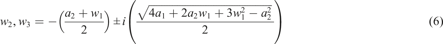
a_{2} = \frac{4 k_{2}}{3 k_{3}} + w_{0}; a_{1} = \frac{2 k_{1}}{k_{3}} + \frac{4 k_{2}}{3 k_{3}} w_{0} + w_{0}^{2}; a_{0} = w_{0}^{3} + \frac{4 k_{2}}{3 k_{3}} w_{0}^{2} + \frac{2 k_{1}}{k_{3}} w_{0} + \frac{4 F}{k_{3}} .

The cubic equation has at least one real solution. This implies that the left hand side of the cubic equation can be expressed generally as a product of one real factor $(w - w_{1})$ and two complex conjugate factors that is $(w - w_{2})$ and $(w - w_{3})$ . The roots of the complex conjugate factors depend on the real root $(w_{1})$ and were derived as:

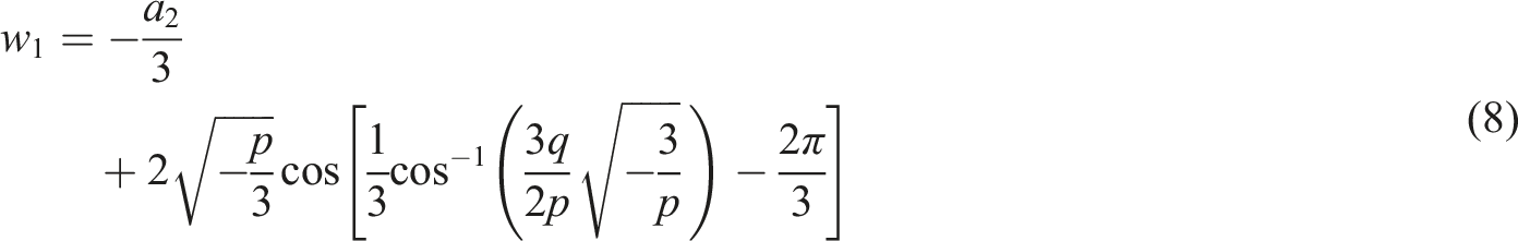
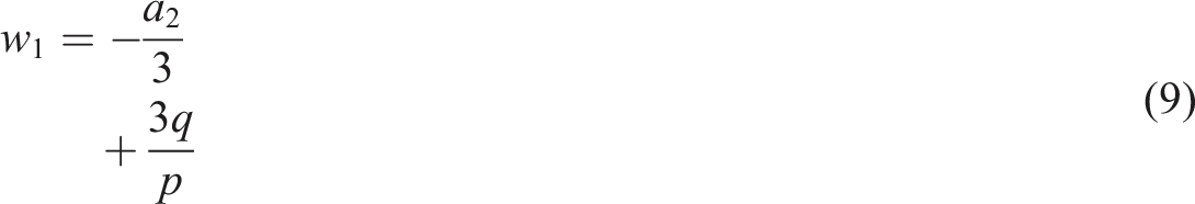
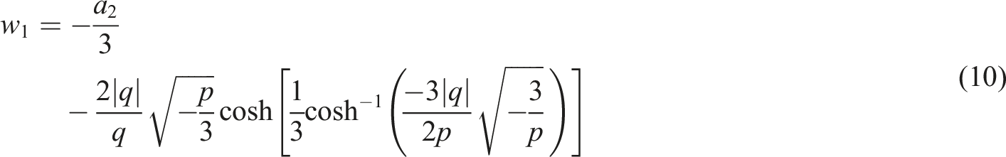
w_{2}, w_{3} = - (\frac{a_{2} + w_{1}}{2}) \pm i (\frac{\sqrt{4 a_{1} + 2 a_{2} w_{1} + 3 w_{1}^{2} - a_{2}^{2}}}{2})

(6)

The real root $(w_{1})$ can be obtained from the depressed form of the cubic equation given as:

x^{3} + p x + q = 0

(7)

where

x = w_{1} + a_{2} / 3

;

p = a_{1} - a_{2}^{2} / 3

and

q = (2 a_{2}^{3} - 9 a_{2} a_{1} + 27 a_{0}) / 27

. The solution to equation (7) depends on the discriminant,

4 p^{3} + 27 q^{2}

, and the value of

p

. Therefore,

w_{1}

can be evaluated based on the following cases⁴:

Case 1

$4 p^{3} + 27 q^{2} < 0$ and $p \neq 0$

w_{1} = - \frac{a_{2}}{3} + 2 \sqrt{- \frac{p}{3}} \cos [\frac{1}{3} \cos^{- 1} (\frac{3 q}{2 p} \sqrt{- \frac{3}{p}}) - \frac{2 π}{3}]

(8)

Case 2

$4 p^{3} + 27 q^{2} = 0$ and $p \neq 0$

w_{1} = - \frac{a_{2}}{3} + \frac{3 q}{p}

(9)

Case 3

$4 p^{3} + 27 q^{2} > 0$ and $p < 0$ ;

w_{1} = - \frac{a_{2}}{3} - \frac{2 | q |}{q} \sqrt{- \frac{p}{3}} \cosh [\frac{1}{3} \cosh^{- 1} (\frac{- 3 | q |}{2 p} \sqrt{- \frac{3}{p}})]

(10)

Case 4

$4 p^{3} + 27 q^{2} > 0$ and $p > 0$

w_{1} = - \frac{a_{2}}{3} - 2 \sqrt{\frac{p}{3}} \sinh [\frac{1}{3} \sinh^{- 1} (\frac{3 q}{2 p} \sqrt{\frac{3}{p}})]

(11)

Case 5

$p = 0$ and $q > 0$

w_{1} = - \frac{a_{2}}{3} - \sqrt[3]{q}

(12)

Case 6

$p = 0$ and $q < 0$

w_{1} = - \frac{a_{2}}{3} + \sqrt[3]{- q}

(13)

Given that all the constants in equation (5) have been defined in terms of the parameters of the HDO and the initial amplitude, we can proceed to determine the period in terms of an elliptic integral. To this end, we apply formula 259.00 on page 133 of Byrd and Friedman²⁴ given as:

\int_{b}^{y} \frac{d z}{\sqrt{(a - z) (z - b) (z - c) (z - \bar{c})}} = G \times F (φ, m)

(14)

where

F (φ, m)

is the incomplete elliptic integral of the first kind defined as:

F (φ, m) = \int_{0}^{φ} {(1 - m \sin^{2} θ)}^{- 1 / 2} d θ

(15)

and the arguments of

F (φ, m)

are defined as follows:

φ = \cos^{- 1} [\frac{(a - y) B - (y - b) A}{(a - y) B + (y - b) A}]

(16a)

m = \frac{{(a - b)}^{2} - {(A - B)}^{2}}{4 A B}

(16b)

Also,

G = \frac{1}{\sqrt{A B}}; A = \sqrt{{(a - r_{2})}^{2} + r_{1}^{2}}; B = \sqrt{{(b - r_{2})}^{2} + r_{1}^{2}}; r_{2} = \frac{c + \bar{c}}{2}; r_{1} = \sqrt{\frac{- {(c - \bar{c})}^{2}}{4}}

(16c)

For direct comparison with the formula in equation (14), the period formula in equation (5) can be rewritten as:

T = 2 \sqrt{\frac{2}{k_{3}}} \int_{w_{0}}^{w_{1}} \frac{d w}{\sqrt{(w_{1} - w) (w - w_{0}) (w - w_{2}) (w - w_{3})}}

(17)

Therefore, $z = w$ , $y = w_{1}$ , $a = w_{1}$ , $b = w_{0}$ , $c = w_{2}$ , $\bar{c} = w_{3}$ . Substituting these results in equations (16a) to (16c) gives:

r_{1} = \frac{1}{2} \sqrt{4 a_{1} + 2 a_{2} w_{1} + 3 w_{1}^{2} - a_{2}^{2}}

(18a)

r_{2} = - (\frac{a_{2} + w_{1}}{2})

(18b)

A = \sqrt{3 w_{1}^{2} + 2 a_{2} w_{1} + a_{1}}

(18c)

B = \sqrt{w_{0}^{2} + w_{0} w_{1} + w_{1}^{2} + a_{2} (w_{0} + w_{1}) + a_{1}}

(18d)

φ = \cos^{- 1} [- 1] = π

(18e)

m = \frac{1}{2} - \frac{3 w_{0} w_{1} + 3 w_{1}^{2} + a_{2} (w_{0} + 3 w_{1}) + 2 a_{1}}{4 \sqrt{3 w_{1}^{2} + 2 a_{2} w_{1} + a_{1}} \sqrt{w_{0}^{2} + w_{0} w_{1} + w_{1}^{2} + a_{2} (w_{0} + w_{1}) + a_{1}}}

(18f)

Consequently, the exact period of the HDO in equation (1) is:

T = 2 \sqrt{\frac{2}{k_{3}}} G \times F (π, m) = 4 \sqrt{\frac{2}{A B k_{3}}} K (m)

(19)

where

A

and

B

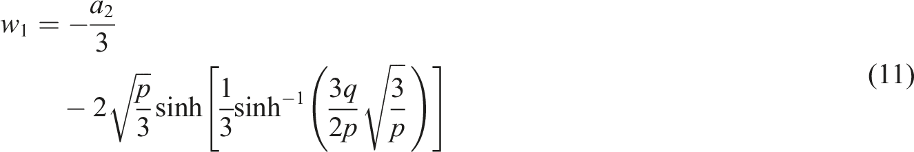
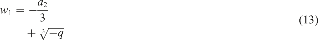
are given in equations (18c,d) and

F (π, m) = 2 K (m)

. Equation (19) can be rewritten in a simplified form as shown:

T = 4 K (m) / ψ

(20)

where

ψ = {[(k_{3} / 2) \sqrt{3 w_{1}^{2} + 2 a_{2} w_{1} + a_{1}} \sqrt{w_{0}^{2} + w_{0} w_{1} + w_{1}^{2} + a_{2} (w_{0} + w_{1}) + a_{1}}]}^{1 / 2}

and

m

is calculated using equation (18f). Note that when

k_{3} < 0

, the expressions in the square roots of

A

and

B

evaluate to negative numbers. The implication is that

A

and

B

will evaluate to complex numbers when

k_{3} < 0

. Therefore, the product

A B

is equal to

\sqrt{3 w_{1}^{2} + 2 a_{2} w_{1} + a_{1}} \sqrt{w_{0}^{2} + w_{0} w_{1} + w_{1}^{2} + a_{2} (w_{0} + w_{1}) + a_{1}}

and should not be evaluated as

\sqrt{(3 w_{1}^{2} + 2 a_{2} w_{1} + a_{1}) (w_{0}^{2} + w_{0} w_{1} + w_{1}^{2} + a_{2} (w_{0} + w_{1}) + a_{1})}

Exact periodic solution of the completely integrable helmholtz-duffing oscillator

In applying the first integral to derive the periodic solution, we considered the integration limits of the RHS of equation (3) to be from $w_{0}$ to $w$ while the corresponding limits for the time integral on the LHS are from $0$ to $t$ . So,

t = \int_{w_{0}}^{w} \frac{d w}{\sqrt{2 F (w_{0} - w) + k_{1} (w_{0}^{2} - w^{2}) + \frac{2}{3} k_{2} (w_{0}^{3} - w^{3}) + \frac{1}{2} k_{3} (w_{0}^{4} - w^{4})}}

(21)

Following the same process as before, the expression in the square root at the denominator of equation (21) can be factorized as:

t = \sqrt{\frac{2}{k_{3}}} \int_{w_{0}}^{w} \frac{d w}{\sqrt{(w_{1} - w) (w - w_{0}) (w - w_{2}) (w - w_{3})}}

(22)

where

w_{1}

w_{2}

and

w_{3}

are already defined in equations (6), and (8–13).

At this point we compare equations (22) and (14) and get: $z = w$ , $y = w$ , $a = w_{1}$ , $b = w_{0}$ , $c = w_{2}$ , $\bar{c} = w_{3}$ . If these results are substituted into equations (16a) to (16c), the results for $A$ , $B$ and $m$ remain the same as in equations (18c,d,f). The only parameter that needs to be re-evaluated is the elliptic amplitude, $φ$ .

φ = \cos^{- 1} [\frac{(a - y) B - (y - b) A}{(a - y) B + (y - b) A}] = \cos^{- 1} [\frac{(w_{1} - w) B - (w - w_{0}) A}{(w_{1} - w) B + (w - w_{0}) A}]

(23a)

which implies that

\cos φ = \frac{(w_{1} - w) B - (w - w_{0}) A}{(w_{1} - w) B + (w - w_{0}) A}

(23b)

Therefore,

t = \sqrt{\frac{2}{k_{3}}} G \times F (φ, m) = \frac{1}{ψ} F (φ, m)

(24)

from which we get

F (φ, m) = ψ t

(25)

The elliptic amplitude can be expressed as the inverse of the incomplete elliptic integral of the first kind that is $φ = F^{- 1} (ψ t, m)$ . Also, the Jacobi cosine function is defined as $\cos φ = \cos [F^{- 1} (ψ t, m)] = cn (ψ t, m)$ . Therefore,

\frac{(w_{1} - w) B - (w - w_{0}) A}{(w_{1} - w) B + (w - w_{0}) A} = cn (ψ t, m)

(26a)

which can be rearranged as:

\frac{w_{0} A + w_{1} B - (A + B) w}{w_{1} B - w_{0} A + (A - B) w} = cn (ψ t, m)

(26b)

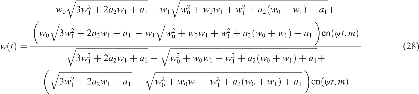
Solving for $w$ in equation (26b) gives the periodic solution of equation (1) as:

w (t) = \frac{w_{0} A + w_{1} B + (w_{0} A - w_{1} B) cn (ψ t, m)}{A + B + (A - B) cn (ψ t, m)}

(27)

Finally, substituting $A$ and $B$ from equations (18c,d) into equation (27) gives:

w (t) = \frac{\begin{array}{c} w_{0} \sqrt{3 w_{1}^{2} + 2 a_{2} w_{1} + a_{1}} + w_{1} \sqrt{w_{0}^{2} + w_{0} w_{1} + w_{1}^{2} + a_{2} (w_{0} + w_{1}) + a_{1}} + \\ (w_{0} \sqrt{3 w_{1}^{2} + 2 a_{2} w_{1} + a_{1}} - w_{1} \sqrt{w_{0}^{2} + w_{0} w_{1} + w_{1}^{2} + a_{2} (w_{0} + w_{1}) + a_{1}}) cn (ψ t, m) \end{array}}{\begin{array}{c} \sqrt{3 w_{1}^{2} + 2 a_{2} w_{1} + a_{1}} + \sqrt{w_{0}^{2} + w_{0} w_{1} + w_{1}^{2} + a_{2} (w_{0} + w_{1}) + a_{1}} + \\ (\sqrt{3 w_{1}^{2} + 2 a_{2} w_{1} + a_{1}} - \sqrt{w_{0}^{2} + w_{0} w_{1} + w_{1}^{2} + a_{2} (w_{0} + w_{1}) + a_{1}}) cn (ψ t, m) \end{array}}

(28)

In contrast to previous exact periodic solutions of the HDO that have been derived using the ansatz approach^5,10,18,19, the present exact periodic solution (equation (28)) was derived naturally from the first integral of the HDO model in equation (1). Furthermore, while the ansatz solutions are limited in the range of parametric conditions that can be solved correctly, the present exact solution has no such limitations and can be applied to obtain the periodic solutions of all possible bounded states as demonstrated in Section 3.

The present exact time period (equation (20)) and periodic solution (equation (28)) are applicable provided that $k_{3} \neq 0$ For the case of $k_{3} = 0$ , the exact solutions derived naturally from the differential equation have been reported by Big-Alabo and Alfred.²⁵ Therefore, the present exact solutions can be used for the following special cases.

a. $F = 0$ and $k_{1} = 0$ : Truly nonlinear HDO

b. $F \neq 0$ and $k_{1} = 0$ : Constantly loaded truly nonlinear HDO

c. $F = 0$ and $k_{2} = 0$ : Duffing oscillator

d. $F \neq 0$ and $k_{2} = 0$ : Constantly loaded Duffing oscillator

e. $F = 0$ , $k_{1} = 0$ and $k_{2} = 0$ : Truly nonlinear Duffing oscillator

f. $F \neq 0$ $k_{1} = 0$ and $k_{2} = 0$ : Constantly loaded truly nonlinear Duffing oscillator

Verification of exact solution

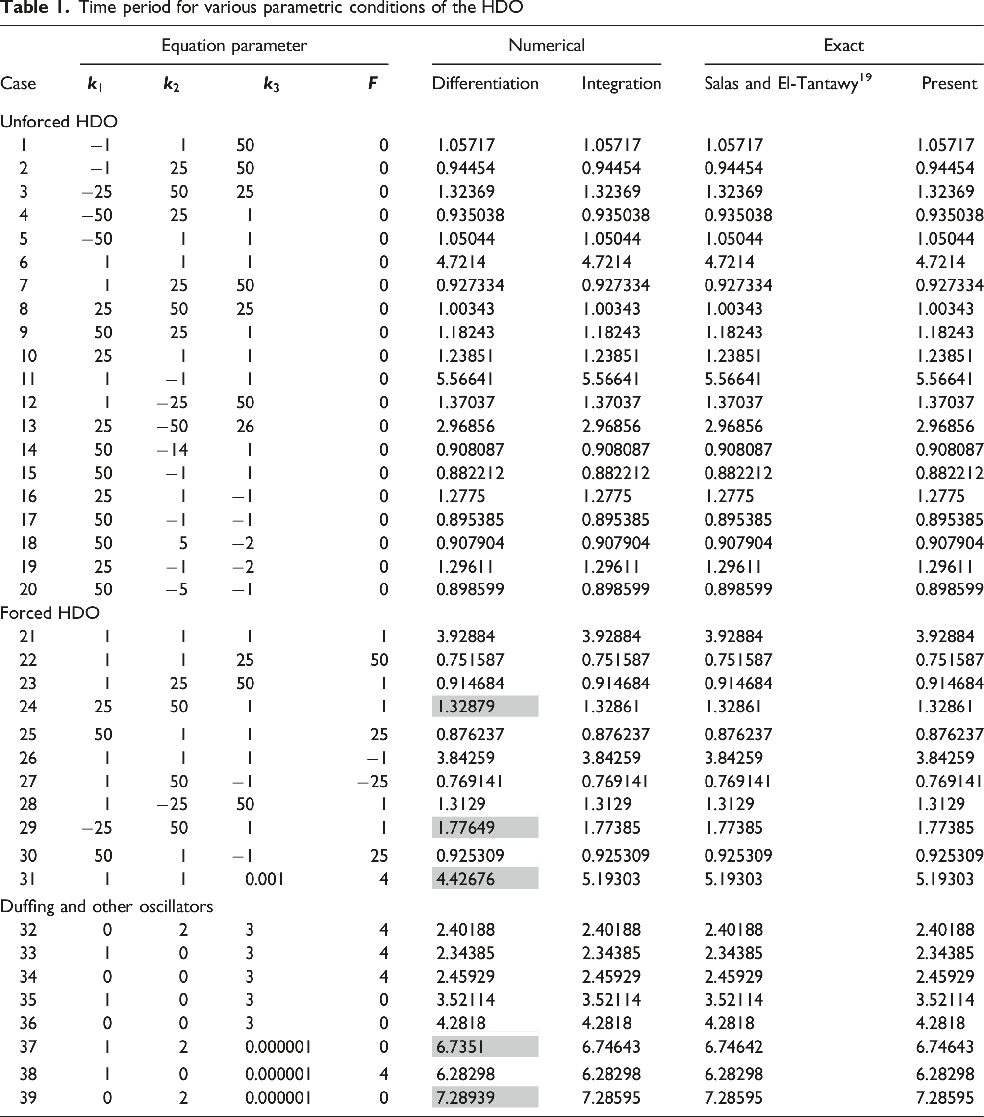
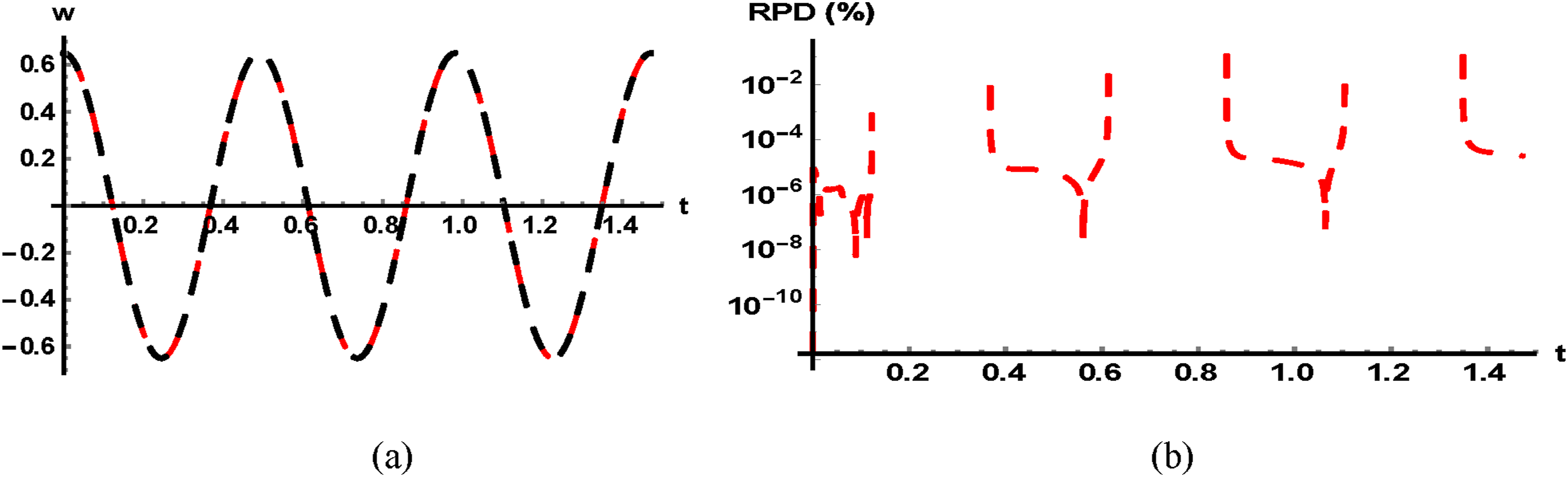
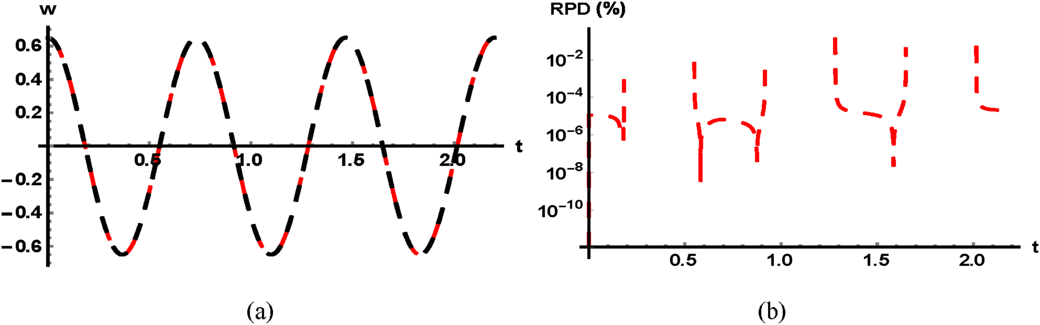
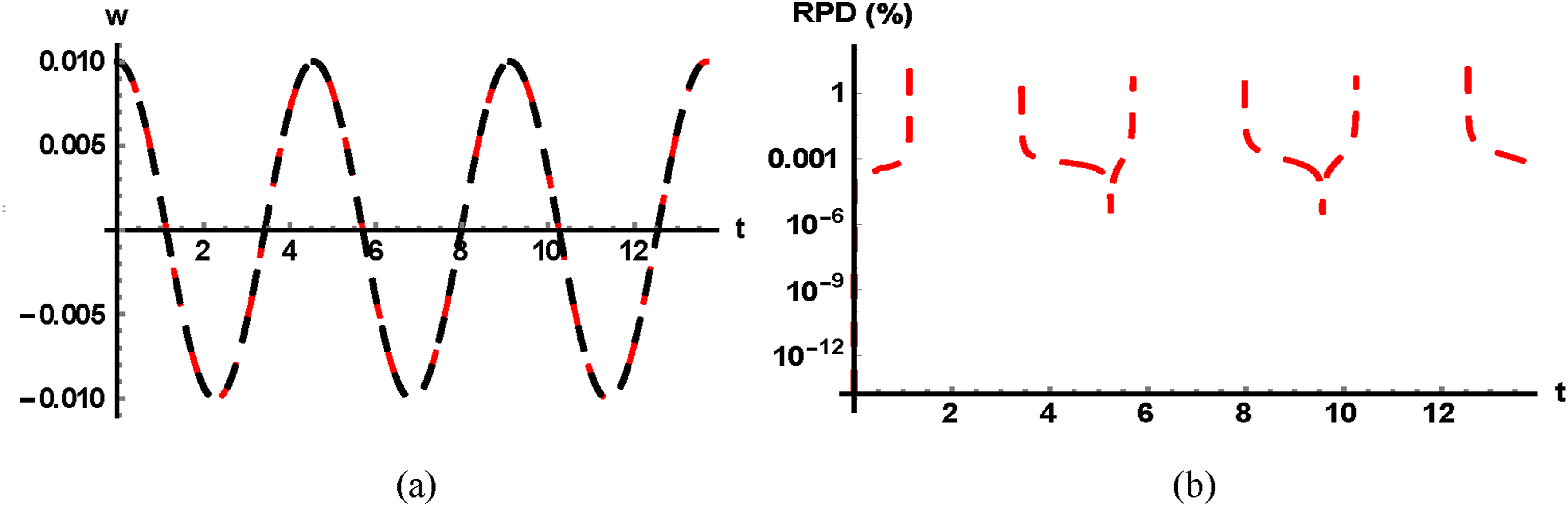
To validate the present exact solutions (equations (20) and (28)) we compared its results with corresponding results of numerical solution and the exact solution of Salas and El-Tantawy¹⁹ – see Appendix C. Both numerical integration and differentiation were considered for the numerical solutions. The numerical integration solutions were obtained by solving equation (4) using the NIntegrate function in Mathematica™ while the numerical differentiation solutions were obtained by solving equation (1) using the NDSolve function in Mathematica™. A wide range of parametric conditions were simulated to demonstrate the validity of the present solution for all bounded states of equation (1). The results of the time period are shown in Table 1, while the displacement solutions are shown in Figure 1. All results were simulated for an initial displacement of 1.0 and the computations and simulations were implemented using Mathematica™.

Table 1.

Time period for various parametric conditions of the HDO

Case	Equation parameter				Numerical		Exact
Case	$k_{1}$	$k_{2}$	$k_{3}$	$F$	Differentiation	Integration	Salas and El-Tantawy¹⁹	Present
Unforced HDO
1	−1	1	50	0	1.05717	1.05717	1.05717	1.05717
2	−1	25	50	0	0.94454	0.94454	0.94454	0.94454
3	−25	50	25	0	1.32369	1.32369	1.32369	1.32369
4	−50	25	1	0	0.935038	0.935038	0.935038	0.935038
5	−50	1	1	0	1.05044	1.05044	1.05044	1.05044
6	1	1	1	0	4.7214	4.7214	4.7214	4.7214
7	1	25	50	0	0.927334	0.927334	0.927334	0.927334
8	25	50	25	0	1.00343	1.00343	1.00343	1.00343
9	50	25	1	0	1.18243	1.18243	1.18243	1.18243
10	25	1	1	0	1.23851	1.23851	1.23851	1.23851
11	1	−1	1	0	5.56641	5.56641	5.56641	5.56641
12	1	−25	50	0	1.37037	1.37037	1.37037	1.37037
13	25	−50	26	0	2.96856	2.96856	2.96856	2.96856
14	50	−14	1	0	0.908087	0.908087	0.908087	0.908087
15	50	−1	1	0	0.882212	0.882212	0.882212	0.882212
16	25	1	−1	0	1.2775	1.2775	1.2775	1.2775
17	50	−1	−1	0	0.895385	0.895385	0.895385	0.895385
18	50	5	−2	0	0.907904	0.907904	0.907904	0.907904
19	25	−1	−2	0	1.29611	1.29611	1.29611	1.29611
20	50	−5	−1	0	0.898599	0.898599	0.898599	0.898599
Forced HDO
21	1	1	1	1	3.92884	3.92884	3.92884	3.92884
22	1	1	25	50	0.751587	0.751587	0.751587	0.751587
23	1	25	50	1	0.914684	0.914684	0.914684	0.914684
24	25	50	1	1	1.32879	1.32861	1.32861	1.32861
25	50	1	1	25	0.876237	0.876237	0.876237	0.876237
26	1	1	1	−1	3.84259	3.84259	3.84259	3.84259
27	1	50	−1	−25	0.769141	0.769141	0.769141	0.769141
28	1	−25	50	1	1.3129	1.3129	1.3129	1.3129
29	−25	50	1	1	1.77649	1.77385	1.77385	1.77385
30	50	1	−1	25	0.925309	0.925309	0.925309	0.925309
31	1	1	0.001	4	4.42676	5.19303	5.19303	5.19303
Duffing and other oscillators
32	0	2	3	4	2.40188	2.40188	2.40188	2.40188
33	1	0	3	4	2.34385	2.34385	2.34385	2.34385
34	0	0	3	4	2.45929	2.45929	2.45929	2.45929
35	1	0	3	0	3.52114	3.52114	3.52114	3.52114
36	0	0	3	0	4.2818	4.2818	4.2818	4.2818
37	1	2	0.000001	0	6.7351	6.74643	6.74642	6.74643
38	1	0	0.000001	4	6.28298	6.28298	6.28298	6.28298
39	0	2	0.000001	0	7.28939	7.28595	7.28595	7.28595

Figure 1.

Displacement solution and error analysis for different parametric conditions of the HDO. Present exact solution – black line, exact solution of Salas and El-Tantawy¹⁹ – blue line, numerical solution – red line.

The results of the time period for the present exact solution, the exact solution of Salas and El-Tantawy¹⁹ and the numerical integration were perfectly matched for all cases. However, the numerical differentiation results showed significant errors in some cases which were highlighted with a gray shade in Table 1 (e.g. case 29 and 31). Similar comparison for the displacement solutions are shown in Figure 1. Also shown in the figure is the relative percentage difference (i.e. $R P D = 100 \times | 1 - w_{p r e s e n t} / w_{o t h e r} |$ ) between the present exact solution and the other solutions. The cases in this figure correspond to those in Table 1. Note that the numerical results in Figure 1 were obtained by solving equation (1) using the NDSolve function in Mathematica. The results show a spike in the RPD at the points where the displacement is zero. This is due to the high sensitivity of the RPD around the zero displacement points and does not affect the accuracy of any of the methods. Therefore, the RPD plots confirm a perfect match between the present exact solution and the exact solution of Salas and El-Tantawy.¹⁹ On the other hand, the numerical solutions show a higher RPD which suggests that the numerical results are generally accurate to seven decimal places except for a few conditions. Cases 24, 29, 31, 37 and 39 represent strong asymmetric nonlinear vibrations. In these cases, the asymmetric response of the HDO with constant load is influenced by two parameters, namely: the quadratic nonlinear stiffness ( $k_{2}$ ) and the constant load ( $F$ ). Higher values of these parameters in relation to the other parameters ( $k_{1}$ and $k_{3}$ ) produce a stronger asymmetric response. It was observed that the numerical solution produced significant errors for cases 24, 29 and 31, whereas it failed to produce displacement solution for cases 37 and 39.

Real-world applications of the helmholtz-duffing oscillator

The HDO has many applications in science and engineering. Here we consider three real-world applications of the HDO and demonstrate the utility of the present exact solutions to solve them.

Functionally-graded microbeam resting on a three-layer nonlinear foundation

The first system that we considered is the vibration of a functionally-graded (FG) microbeam resting on a three-layer elastic foundation consisting of Winkler, Pasternak and nonlinear stiffness. FG microbeams have application in the production of MEMS devices used in thermally elevated environment for example in electronic components. The vibration model for an FG microbeam with pin-pin boundary conditions and resting on a three-layer nonlinear foundation was derived by Alfred et al⁴ and can be expressed as:

\frac{d^{2} Q}{d t^{2}} + γ_{1} Q + γ_{2} Q^{2} + {γ_{3} Q}^{3} = γ_{4}

(29)

where

Q

is the dimensionless displacement of the functionally-graded microbeam and the initial conditions are

Q (0) = Q_{0}

and

\dot{Q} (0) = 0

. The expressions to evaluate the linear and nonlinear stiffness constants (

γ_{1}

γ_{2}

γ_{3}

) and the constant load (

γ_{4}

) are given in Appendix A. Under clamp-clamp boundary conditions,

γ_{2} = 0

and the FG microbeam only experiences a symmetric vibration response. For pin-pin boundary conditions

γ_{2} \neq 0

and the FG microbeam can exhibit a strong asymmetric vibration response. To demonstrate this, we consider typical properties of a steel-ceramic FG microbeam as shown in Tables 2 and 3. The dimensions of the microbeam are: length,

L = 20 h

; length scale ratio,

μ / h = 0.25

; breadth and thickness,

b = h = 5.0 \times 10^{- 6} m

. The dimensionless foundation parameters were taken as

κ_{n} = κ_{s} = κ_{l} = 1.0

and

Q_{0} = 1.0

Table 2.

Mechanical properties of steel-ceramic components at room temperature.

S/N	Steel (SUS304)		Alumina (Al₂O₃)
S/N	Property	Value	Property	Value
1	$E_{1}$	$210 G P a$	$E_{2}$	$390 G P a$
2	$v_{1}$	0.3177	$v_{2}$	0.3
3	$ρ_{1}$	$8166 k g / m^{3}$	$ρ_{2}$	$3960 k g / m^{3}$
4	$α_{1}$	$15.321 \times 10^{- 6} K^{- 1}$	$α_{2}$	$7.475 \times 10^{- 6} K^{- 1}$

Table 3.

Temperature dependent coefficients of FG microbeam property.

Material	Property	$P_{0}$	$x_{0}$	$x_{1}$	$x_{2}$	$x_{3}$
STEEL	E	$201.04 G P a$	$0$	$3.08 \times 10^{- 4}$	$- 6.53 \times 10^{- 7}$	0
	$v$	0.3262	0	$- 2.0 \times 10^{- 4}$	$3.80 \times 10^{- 7}$	0
	$α$	$1.233 \times 10^{- 5} K^{- 1}$	0	$8.09 \times 10^{- 4}$	$0$	0
	$ρ$	8166 $k g / m^{3}$	0	0	0	0
Ceramics	E	$348.43 G P a$	$0$	$- 3.07 \times 10^{- 4}$	$2.16 \times 10^{- 7}$	$- 8.95 \times 10^{- 11}$
	$v$	0.3	0	0	0	0
	$α$	$5.87 \times 10^{- 6} K^{- 1}$	0	$9.10 \times 10^{- 4}$	0	0
	$ρ$	3960 $k g / m^{3}$	0	0	0	0

FG microbeam at room temperature subjected to constant load

The difference in temperature of the two materials that make up the functionally graded microbeam is equal to zero at room temperature that is $∆ T = T_{1} - T_{2} = 0$ . Also, we assume that $F = 100 N / m$ . The constants $γ_{1}$ , $γ_{2}$ , $γ_{3}$ and $γ_{4}$ were evaluated as: $γ_{1} = 68.6603$ , $γ_{2} = - 7.77938$ , $γ_{3} = 25.1023$ , and $γ_{4} = 637.9$ . In comparison to equation (1), $k_{1} = γ_{1}$ , $k_{2} = γ_{2}$ , $k_{3} = γ_{3}$ and $F = γ_{4}$ . Therefore, the period obtained for the present exact solution is $T_{e x} = 0.3064420571089396$ while that for numerical integration is $T_{N I} = 0.30644205712344297$ . The results show that the present exact solution and the numerical solution match to 10 decimal places. The displacement response and the RPD of the numerical solution in comparison to the present exact solution are shown in Figure 2. It can be observed that the present exact solution and the numerical solution match excellently. The FG microbeam exhibits a strong asymmetric response and demonstrates that a small initial displacement can lead to significantly large biased amplitude that is a multiple of the initial displacement. An accurate estimation of the biased amplitude and the displacement profile is necessary to inform design considerations in the optimal placement of MEMS devices made up of FG microbeams.

Figure 2.

(a) Displacement response of FG microbeam at room temperature: black – present exact solution, red – numerical solution (b) RPD plot for numerical solution.

FG microbeam vibrating at near buckling thermal load

Since FG microbeams are particularly suited for thermally elevated environments, we considered the scenario for which $∆ T = 155.9$ °C and $F = 0.0 N / m$ . The stiffness constants and constant force were computed as: $γ_{1} = - 7.66654$ , $γ_{2} = - 7.3402$ , $γ_{3} = 25.1294$ , and $γ_{4} = 0.0$ . The conditions of the FG microbeam analysed here are those of a near buckling vibration since the buckling temperature is $∆ T = 155.909$ °C. Using these results, the period and frequency of the present exact solution were calculated as 6.943691544727408 and 0.9048767887667234 respectively. The corresponding results of the numerical integration method are the same as those of present exact solution which shows that both solution match to 15 decimal places. The displacement response (see Figure 3) of the near buckling vibration is a strong anharmonic asymmetric response indicating the existence of strong nonlinear restoring forces at work. This kind of response is usually not predicted accurately by most approximate analytical methods for solving the HDO. The RPD of the numerical solution reveals that the numerical solution was accurate to about 4 decimal places. The near buckling condition is an example of a highly stiff nonlinear ODE for which numerical differentiation methods are generally known to have a reduced accuracy compared to non-stiff ODEs. It can be observed that the biased amplitude ( $w_{1}$ ) is less than the initial amplitude due to the quadratic nonlinear effect induced by the boundary conditions. The FG microbeam is highly stiff due to the high thermal gradient across its thickness. At near buckling temperature, the stiffness of the beam causes a strong anharmonic profile in the vibration response that results to a slower response time. Since typical applications of the FG microbeam as actuators and sensors require fast response times, it is important to avoid operating the FG microbeam at near buckling temperature. Furthermore, cooling of the FG microbeam by means of a blower is important for optimal functionality.

Figure 3.

(a) Near buckling displacement response of FG microbeam: black – present exact solution, red – numerical solution (b) RPD plot for numerical solution.

Vibration of a hyper-elastic beam resting on nonlinear hardening elastic foundation

Hyper-elastic materials are rubberlike materials that a capable of large strains under various loading conditions. Due to their constitutive behaviours, they find applications in biological systems and soft mechanical structures.^26,27 Forsat²⁷ investigated the free nonlinear vibration of a simply-supported hyper-elastic beam resting on nonlinear hardening elastic foundation. The vibration model for the hyper-elastic beam was derived as follows:

M \ddot{W} + (K_{33} + T_{3}) W + (G_{4} T_{1} + G_{5} T_{3} + T_{4}) W^{2} + (G_{3} + G_{4} T_{2} + G_{5} T_{4}) W^{3} = 0

(30)

where the initial conditions are:

W (0) = W_{0}, \dot{W} (0) = 0

. The expression for the parameters in equation (30) are given in Appendix B. Forsat²⁷ investigated four different hyper-elastic material models and observed that the Ishihara hyper-elastic model provided a better prediction of the constitutive behaviour compared to the other three models. Hence, we apply the Ishihara hyper-elastic model. The properties of silicon rubber and unfilled natural rubber based on this model are shown in Table 4. The constants

c_{10}

c_{01}

, and

c_{20}

in Table 4 are the Ishihara hyper-elastic model parameters, and

ρ

is the density. The dimensions of the hyper-elastic beam were taken as: length,

L = 10 h

, breadth,

b = 2 h

and thickness,

h = 0.65 m

. The values of the Wrinkler, Pasternak and nonlinear foundation parameters were taken as:

κ_{w} = 200

κ_{p} = 20

, and

κ_{n l} = 100

respectively, and

W_{0} = 0.65

Table 4.

Hyper-elastic beam model parameters.

S/N	SILICON rubber		UNFILLED natural rubber
S/N	Property	Value	Property	Value
1	$c_{10}$	$315571 Pa$	$c_{10}$	$116100 Pa$
2	$c_{01}$	−5931.41 Pa	$c_{01}$	11400 Pa
3	$c_{20}$	66929.04 Pa	$c_{20}$	13600 Pa
4	$ρ$	$1100 k g / m^{3}$	$ρ$	$1060 k g / m^{3}$

Silicon rubber hyper-elastic beam

Using the data in Table 4 and the equations in Appendix B the parameters in equation (30) were computed as $M = 2342.86$ , $K_{33} = 364624$ , $T_{1} = 0.0$ , $T_{2} = - 0.4244$ , $T_{3} = 0.395962$ , $T_{4} = 0.0$ , $G_{3} = 51155.4$ , $G_{4} = - 26196.1$ , $G_{5} = 0.0$ . In comparison to equation (1), $k_{1} = (K_{33} + T_{3}) / M = 155.632$ , $k_{2} = (G_{4} T_{1} + G_{5} T_{3} + T_{4}) / M = 0.0$ , $k_{3} = (G_{3} + G_{4} T_{2} + G_{5} T_{4}) / M = 26.580$ , and $F = 0.0$ . The frequency obtained using the present exact solution was 4.915089139144477 while frequency obtained from numerical solution is 4.915089156828689. Both frequency results match to 7 decimal places. The displacement response comparing the present exact solution and numerical solution are shown in Figure 4(a) while the RPD of the numerical solution is shown in Figure 4(b). The figure confirms the excellent agreement between the present exact solution and the numerical solution. It can be observed that the displacement profile for this example is symmetric. This is because the coefficient of the quadratic nonlinear stiffness is zero. Moreover, the displacement profile appears to be harmonic due to the small initial displacement. Therefore, the effect of the nonlinearities for this example is not significant and the system’s vibration response can be accurately predicted by an equivalent linear oscillator.

Figure 4.

(a) Displacement response of silicon rubber hyper-elastic beam: black – present exact solution, red – numerical solution (b) RPD plot for numerical solution.

Unfilled natural rubber hyper-elastic beam

Again using the data in Table 4 and the equations in Appendix B the parameters in equation (30) were computed for the unfilled natural rubber beam as $M = 2342.86,$ $K_{33} = 160599$ , $T_{1} = 0.0$ , $T_{2} = - 0.424413$ , $T_{3} = - 0.063802$ , $T_{4} = 0.0$ , $G_{3} = 15008,$ $G_{4} = - 5323.05$ , and $G_{5} = 0.0$ . Hence, $k_{1} = 68.5482$ , $k_{2} = 0.0$ , $k_{3} = 7.37013$ and $F = 0.0$ . The frequencies computed using the present exact solution and numerical solution are $5.326680342510904$ and $5.326680361846545$ respectively. The frequency estimates of both methods match up to 7 decimal places. For the same conditions of vibration, the unfilled natural rubber beam has a higher frequency compared to the silicon rubber beam, which implies that it has a higher effective stiffness. Therefore, we can conclude that the unfilled natural rubber beam experiences less strain during vibration compared to a silicon rubber beam under the same conditions. Figure 5 shows the periodic solutions for both methods together with the RPD of the numerical solution. The error of the numerical solution is negligible.

Figure 5.

(a) Displacement response of unfilled natural rubber hyper-elastic beam: black – present exact solution, red – numerical solution (b) RPD plot for numerical solution.

Vibration of optomechanical system

The interaction of light with matter in some material leads to mechanical effects which have practical applications. Systems of this nature are called optomechanical systems and they are usually modelled as oscillators coupled to an optical cavity with nonlinear connection. Assuming that both linear and quadratic connections are present, the dynamic equation of the optomechanical system under adiabatic conditions is given as³:

\ddot{x} + (1 + 4 I ω_{2}) x + 2 I ω_{1} = 0

(31)

where

ω_{1}

is the linear connection parameter,

ω_{2}

is the nonlinear connection parameter, and

I

is the interactivity field expressed as:

I (t) = 2 δ_{c} Γ^{2} (ω_{1} x - ω_{2} x^{2}) = 0

(32)

where

Γ = η / [{(ζ / 2)}^{2} + δ_{c}^{2}]

η

is the amplitude related to the input optic power,

ζ

is the damping rate,

δ_{c} = ω_{0} - ω_{p}

is the cavity-pump detuning,

ω_{0}

is the resonance frequency, and

ω_{p}

is the frequency of energy pumping. Substituting equation (32) into (31) gives:

\ddot{x} + (1 + 4 ω_{1}^{2} δ_{c} Γ^{2}) x + (4 ω_{1} ω_{2} δ_{c} Γ^{2}) x^{2} - (8 ω_{2}^{2} δ_{c} Γ^{2}) x^{3} = 0

(33)

To simulate the periodic solution of equation (33) we apply typical experimental values reported by Cveticanin et al³ as follows: $η = 31.623$ , $ζ = 2$ , $δ_{c} = 1$ , $ω_{1} = 0.03$ and $ω_{2} = 0.03333$ . Additionally, the initial conditions considered are $x (0) = 0.01$ and $\dot{x} (0) = 0.0$ . The stiffness constants were obtained from equation (33) as $k_{1} = 1.9$ , $k_{2} = 0.9999$ , and $k_{3} = - 2.2217778$ . Therefore, the coefficients of the cubic equation used in the present exact solution were computed as $a_{2} = - 0.5900600$ , $a_{1} = - 1.716242651$ and $a_{0} = - 0.01716242651$ . The coefficients of the corresponding depressed cubic equation were determined as $p = - 1.832 < 0$ and $q = - 0.369942 < 0$ , which implies that the discriminant of the depressed cubic is $4 p^{3} + 27 q^{2} = - 20.9113 < 0$ . Then, $w_{1}$ was determined from the equation (8) as $- 0.0100352123$ . The value of $w_{1}$ suggests that the periodic oscillation is almost symmetric (see Figure 6). The completely integrable HDO exhibits a symmetric oscillation when $k_{2} = 0$ and $F = 0$ . In this example, $F = 0$ but $k_{2} \neq 0$ . However, $k_{1}$ and $k_{3}$ are about twice the magnitude of $k_{2}$ . Additionally, the oscillation amplitude is small. Hence, the combined effect of the small-amplitude and relative magnitudes of the stiffness constants makes the asymmetric effect to be insignificant in this example.

Figure 6.

(a) Displacement response of optomechanical system: black – present exact solution, red – numerical solution (b) RPD plot for numerical solution.

The solution parameters $A$ , $B$ and $m$ were calculated as $A = 1.30541 i$ , $B = 1.3100 i$ and $m = - 0.00006177$ . Substituting these results in equation (19) give the value of the present exact period as $T_{e x} = 4.558555125950275$ . The corresponding period estimate obtained by numerical integration was $T_{N I} = 4.5585574961819555$ and matches to 5 decimal places compared to the exact solution. The details of the values of the constants in the present exact solution were discussed in this example because they illustrate the point made earlier about evaluating the product of the square roots, $A$ and $B$ . In this example, the product ( $A \times B$ ) is negative and this make the square root in equation (19) evaluate to a real value since $k_{3} < 0$ . If on the other hand, the square roots $A$ and $B$ are combined into a single square root before evaluating, then equation (19) will evaluate to a complex number and we will not get the correct period. Figure 6 shows the periodic solutions for the exact and numerical solutions together with the RPD of the numerical solution. The RPD results show that the numerical solution is at least accurate to three significant figures. Due to the sinusoidal nature of the oscillation profile, the optomechanical system is exhibiting a weakly nonlinear vibration response that can be accurately predicted by perturbation theory. However, it is possible for the system to exhibit conditions of strong nonlinear vibration with asymmetric response.

Conclusion

The Helmholtz-Duffing oscillator (HDO) is a fundamental model that governs the vibration of many systems in science and engineering. Several approximate and exact analytical solutions have been derived for the time period or frequency and periodic solution of the HDO. While the approximate solutions are capable of predicting the weak and moderately nonlinear response of the HDO, they produce large errors for the strong nonlinear response of the HDO. The strong nonlinear response is responsible for symmetry-breaking and pull-in/down instability phenomena and is important for predicting the near bucking vibrations of beams. On the other hand, the published exact solutions of the HDO are usually derived based on the ansatz approach and have various limits in the range of bounded oscillations they can solve.¹⁰ The only possible exception is the exact solution of Salas and El-Tantawy¹⁹ that was derived based on an ansatz solution in the form of Weierstrass elliptic function. However, the range of validity of the ansatz solution of Salas and El-Tantawy¹⁹ is yet to be tested and the solution is quite complicated compared to the solutions in the form of Jacobi elliptic function. Moreover, the ansatz approach forces the solution to take a predetermined form as opposed to the actual form.

A major drawback of the ansatz approach is that the derived exact solution has a limited range of validity and does not apply to all cases of bounded periodic conditions. The present study applies a different approach to the existing studies by deriving the exact solution of the HDO naturally from the first integral of the differential equation. A general form of the completely integrable undamped HDO having arbitrary stiffness constants and a constant force was considered and solved exactly. The time period solution was derived in terms of the complete elliptic integral of the first kind and the periodic solution was derived in terms of the Jacobi cosine function. Interestingly, the present exact solutions (time period and displacement) are applicable to all possible bounded states of the HDO as identified by Geng.¹⁰ By comparing the results of the present exact solutions with corresponding results of numerical solutions and the exact solutions of Salas and El-Tantawy,¹⁹ the validity of the present exact solutions was confirmed. Nevertheless, the results demonstrate that the numerical differentiation solution, which is commonly used to verify the accuracy of approximate periodic solutions, can produce significant errors under certain parametric conditions. This underscores the necessity of the present exact solutions. Given the straightforward manner in which the present exact solutions were derived, they can be readily implemented in a simple computer program in MatLab or Mathematica for any kind of periodic analysis of the completely integrable HDO. Consequently, we recommend the present exact time period and displacement solution as benchmark solutions that could be used to determine the accuracy of other approximate solutions. Additionally, the application of the present exact solution to analyse real-world problems was demonstrated using two types of beam system and an optomechanical system.

In terms of future work, the present exact displacement solution can be applied to investigate the periodic response of the damped and forced HDO. This can be achieved by multiplying the present exact solution with an exponential function having an unknown constant that accounts for damping. The constant can be determined from the residual function of the governing differential equation.²⁰ Such approximate solution can be used to investigate jump phenomenon, softening/hardening backbone response, bifurcation analysis and chaotic behaviour. Another area where the utility of the present exact solutions may be explored is in the derivation of an equivalent oscillator to investigate the asymmetric response of nonlinear systems with complicated non-polynomial restoring force. This can be achieved by applying the principle of quasi-static equilibrium.²⁸ However, in a scenario where the inputs are characterised by uncertainties, approximate stochastic methods for solving nonlinear differential equations, such as Artificial Neural Network²⁹ or Deep Neural Network,³⁰ could be applied to investigate the response of the HDO.

Footnotes

Author Contribution

Dr A. Big-Alabo – Conceptualization, methodology, results, writing and proof-reading. Mr P.A. Alfred – Methodology, simulation, results, writing and proof-reading.

Declaration of conflicting interests

The author(s) declared no potential conflicts of interest with respect to the research, authorship, and/or publication of this article.

Funding

The author(s) received no financial support for the research, authorship, and/or publication of this article.

ORCID iDs

Akuro Big-Alabo

Peter B Alfred

Appendix A

The expressions to evaluate the linear and nonlinear stiffness parameters and the constant load parameter of equation (29) are given as⁴: (A1)

γ_{1} = \frac{1}{a_{1}} (β \int_{0}^{1} φ \frac{\partial^{4} φ}{\partial {\bar{x}}^{4}} d \bar{x} + η_{1} \int_{0}^{1} φ \frac{\partial^{3} φ}{\partial {\bar{x}}^{3}} d \bar{x} + κ_{l} \int_{0}^{1} φ^{2} d \bar{x} + (μ_{T} - κ_{s}) \int_{0}^{1} φ \frac{\partial^{2} φ}{\partial {\bar{x}}^{2}} d \bar{x})

(A2)

γ_{2} = \frac{η_{3}}{a_{1}} \int_{0}^{1} (\frac{\partial^{2} φ}{\partial {\bar{x}}^{2}}) d \bar{x} \int_{0}^{1} φ \frac{\partial^{2} φ}{\partial {\bar{x}}^{2}} d \bar{x}

(A3)

γ_{3} = \frac{1}{a_{1}} (η_{4} \int_{0}^{1} [{φ (\frac{\partial φ}{\partial \bar{x}})}^{3}] d \bar{x} - η_{2} \int_{0}^{1} [\frac{r}{2} {(\frac{\partial φ}{\partial \bar{x}})}^{2}] d \bar{x} \int_{0}^{1} φ \frac{\partial^{2} φ}{\partial {\bar{x}}^{2}} d \bar{x} + κ_{n} \int_{0}^{1} φ^{4} d \bar{x})

(A4)

γ_{4} = \frac{1}{a_{1}} \int_{0}^{1} \bar{F} φ d \bar{x}

where (A5a)

a_{1} = \int_{0}^{1} φ^{2} d \bar{x} - \frac{I_{3}}{I_{1} L} \int_{0}^{1} φ \frac{\partial^{2} φ}{\partial {\bar{x}}^{2}} d \bar{x}

and the shape function for pin-pin boundary condition is: (A5b)

φ (\bar{x}) = \sin (π \bar{x})

Also, (A6)

{I_{1}, I_{2}, I_{3}} = b \int_{- h / 2}^{+ h / 2} ρ {1, z, z^{2}} d z

The dimensionless parameters in equations (A1–A4) are defined as equation (A7): (A7)

\bar{x} = \frac{x}{L}; \bar{w} = \frac{w}{r}; r = \sqrt{\frac{I}{A}}; β = | 1 + (\frac{H}{D} - \frac{B^{2}}{A D}) |; {η_{1} = \frac{B^{2}}{A D}; η}_{2} = \frac{A r}{D}; η_{3} = \frac{B r}{D}; η_{4} = \frac{- A r^{2}}{2 D}; κ_{l} = \frac{K_{L} L^{4}}{D}; μ_{T} = \frac{N_{T} L^{2}}{D}; κ_{s} = \frac{K_{S} L^{2}}{D}; κ_{n} = \frac{K_{N} r^{2} L^{4}}{D}; t = \bar{t} \sqrt{\frac{I_{1} L^{4}}{D}}; \bar{F} = \frac{F L^{4}}{r D}

where

L

b

and

h

are the length, breadth and height of the beam respectively,

A = b h

I

is the moment of inertia of the beam cross-section,

ρ

is the mass density of the microbeam,

κ_{l}

is the dimensionless Winkler parameter,

κ_{s}

is the dimensionless Pasternak parameter,

κ_{n}

is the dimensionless nonlinear foundation parameter,

\bar{F}

is the dimensionless load, and

F

is the normal distributed load.

K_{L}

K_{S}

and

K_{N}

are the Winkler, Pasternak and nonlinear foundation stiffness, whereas

t

is time and

w

is the displacement.

The parameters defining the thermo-elastic constitutive behaviour of the FG microbeam are evaluated as: (A8)

{A, B, D} = b \int_{- h / 2}^{+ h / 2} E {1, z, z^{2}} d z

(A9)

H = b \int_{- h / 2}^{+ h / 2} \frac{E μ^{2}}{2 (1 + v)} d z

(A10)

N_{T} = b \int_{- h / 2}^{+ h / 2} E α ∆ T d z

where

∆ T = T_{1} - T_{2}

is the temperature difference between the two materials M1 and M2, while

α

is the temperature-dependent coefficient of thermal expansion. The material properties are defined as: (A11)

P = (P_{1} - P_{2}) {(\frac{z}{h} + \frac{1}{2})}^{n} + P_{2}

(A12)

T (z) = (T_{1} - T_{2}) (\frac{z}{h} + \frac{1}{2}) + T_{2}

(A13)

P (T) = P_{0} (1 + \frac{x_{0}}{T} + x_{1} T + x_{2} T^{2} + x_{3} T^{3})

Therefore, the thermo-spatial properties, $P (z, T)$ , of the FG material can be represented as: (A14)

P (z, T) = [P_{1} (T (z)) - P_{2} (T (z))] {(\frac{z}{h} + \frac{1}{2})}^{n} + P_{2} (T (z))

from which the thermo-elastic properties are determined as: (A15a)

E = [E_{1} (T (z)) - E_{2} (T (z))] {(\frac{z}{h} + \frac{1}{2})}^{n} + E_{2} (T (z))

(A15b)

ν = [v_{1} (T (z)) - v_{2} (T (z))] {(\frac{z}{h} + \frac{1}{2})}^{n} + v_{2} (T (z))

(A15c)

ρ = (ρ_{1} - ρ_{2}) {(\frac{z}{h} + \frac{1}{2})}^{n} + ρ_{2}

(A15d)

α = [α_{1} (T (z)) - α_{2} (T (z))] {(\frac{z}{h} + \frac{1}{2})}^{n} + α_{2} (T (z))

where

n

is a non-negative power law index,

P = {E, v, ρ, and α}

E, v, ρ, and α

are the effective Young’s modulus, Poisson ratio, density and coefficient of thermal expansion. The subscripts 1 and 2 represent the properties for materials M1 and M2.

Appendix B

The parameters in equation (30) were evaluated as²⁷: (B1)

M = I_{0} \int_{0}^{L} φ^{2} d z - I_{2} \int_{0}^{L} φ^{″} φ d z

(B2)

G_{1} = - {8 A}_{x x} C_{20} \int_{0}^{L} φ^{″} {(φ^{'})}^{2} d z

(B3)

G_{2} = - {8 E}_{x x} C_{20} \int_{0}^{L} φ^{″} {(φ^{'})}^{2} d z

(B4)

G_{3} = - {12 A}_{x x} C_{20} \int_{0}^{L} φ^{″} {(φ^{'})}^{2} φ d z + k_{n} \int_{0}^{L} φ^{4} d z

(B5)

G_{4} = - {8 A}_{x x} C_{20} (\int_{0}^{L} {(φ^{″})}^{2} φ d z + \int_{0}^{L} φ^{‴} φ^{'} φ d z)

(B6)

G_{5} = - {8 E}_{x x} C_{20} (\int_{0}^{L} {(φ^{″})}^{2} φ d z + \int_{0}^{L} φ^{‴} φ^{'} φ d z)

(B7)

T_{1} = \frac{K_{21} K_{32}}{K_{11} K_{22} - K_{12} K_{21}}

(B8)

T_{2} = \frac{G_{2} K_{21} - G_{1} K_{22}}{K_{11} K_{22} - K_{12} K_{21}}

(B9)

T_{3} = \frac{{- K}_{11} K_{32}}{K_{11} K_{22} - K_{12} K_{21}}

(B10)

T_{4} = \frac{G_{1} K_{12} - G_{2} K_{11}}{K_{11} K_{22} - K_{12} K_{21}}

(B11)

K_{11} = - {8 A}_{x x} C_{20} \int_{0}^{L} φ^{‴} φ^{'} d z

(B12)

K_{12} = K_{21} = - {8 E}_{x x} C_{20} \int_{0}^{L} φ^{‴} φ^{'} d z

(B13)

K_{22} = - 2 \tilde{F} C_{01} \int_{0}^{L} φ^{'} φ^{'} d z - {8 C_{20} H}_{x x} \int_{0}^{L} φ^{‴} φ^{'} d z

(B14)

K_{32} = {8 F}_{x x} C_{20} \int_{0}^{L} φ^{‴} φ^{'} d z

(B15)

K_{23} = - 8 F_{x x} C_{20} \int_{0}^{L} φ^{⁗} φ d z

(B16)

K_{33} = - {2 A}_{x x} (C_{10} + 2 C_{01}) \int_{0}^{L} φ^{″} φ d z + {8 D}_{x x} C_{20} \int_{0}^{L} φ^{⁗} φ d z + k_{w} \int_{0}^{L} φ^{2} d z - k_{p} \int_{0}^{L} φ^{″} φ d z

where

φ (x)

this is the shape function which is dependent on the boundary conditions,

C_{10}

C_{01}

, and

C_{20}

are the Ishihara hyper-elastic model parameters, and

z

is the distance of any point along the thickness axis. The shape function for the fundamental vibration mode under simply-supported boundary conditions is: (B17)

φ (x) = \sin (\frac{π x}{L})

The parameters describing the constitutive behaviour of the hyper-elastic beam are given as: (B18)

{I_{0}, I_{2}} = \int_{- h / 2}^{+ h / 2} ρ {1, z^{2}} d z

and (B19)

{A_{x x}, D_{x x}, E_{x x}, F_{x x}, H_{x x}} = \int_{- h / 2}^{+ h / 2} {1, z^{2}, f, z f, f^{2}} d z

where

f (z)

is the shear distribution function given as: (B20)

f (z) = \frac{h}{z} Sin (\frac{π z}{h})

Appendix C

Salas and El-Tantawy¹⁹ derived an exact solution of equation (1) with initial conditions $w (0) = w_{0}$ and $\dot{w} (0) = {\dot{w}}_{0}$ using an ansatz solution in the form of Weierstrass elliptic function ( $℘$ ). For the case of $F = 0$ , they assumed the following exact periodic solution: (C1)

w (t) = (A + \frac{B}{1 + C ℘ (t + t_{0}; g_{2}, g_{3})})

Equation (C1) has six unknown solution parameters ( $A$ , $B$ , $C$ , $g_{2}$ , $g_{3}$ , and $t_{0}$ ) that were derived as: (C2)

B = - \frac{6 A (k_{1} + A (k_{2} + A k_{3}))}{k_{1} + A (2 k_{2} + 3 A k_{3})}

(C3)

C = \frac{12}{k_{1} + 2 A k_{2} + 3 A^{2} k_{3}}

(C4)

g_{2} = \frac{1}{12} (k_{1}^{2} - 6 A^{2} k_{1} k_{3} - A^{3} k_{3} (4 k_{2} + 3 A k_{3}))

(C5)

g_{3} = \frac{1}{216} (k_{1}^{3} + 18 A^{2} k_{1}^{2} k_{3} - A^{3} k_{2}^{2} (4 k_{2} + 3 A k_{3}) + 3 A^{2} k_{1} (- 2 k_{1}^{2} + 4 A k_{2} k_{3} + 3 A^{2} k_{3}^{2}))

(C6)

t_{0} = \pm ℘^{- 1} (\frac{w_{0} - A - B}{C (A - w_{0})}; g_{2}, g_{3})

whereas

A

is the root to the quartic equation (C7)

3 A^{4} k_{3} + 4 A^{3} k_{2} + 6 A^{2} k_{1} - 6 k_{1} w_{0}^{2} - 4 k_{2} w_{0}^{3} - 3 k_{3} w_{0}^{4} - 6 {\dot{w}}_{0}^{2} = 0

For the case of $F \neq 0$ , they expressed the exact periodic solution as: (C8)

w (t) = y (t) + ζ

where

ζ

is the particular solution and

y (t)

is the exact solution to the transformed unforced equation given as: (C9)

\ddot{y} + (k_{1} + 2 k_{2} ζ + 3 k_{3} ζ^{2}) y + (k_{2} + 3 k_{3} ζ) y^{2} + k_{3} y^{3} = 0

and subject to the initial conditions,

y (0) = w_{0} - ζ

and

\dot{y} (0) = {\dot{w}}_{0}

The particular solution $ζ$ was derived as the root of the following cubic equation: (C10)

k_{3} ζ^{3} + k_{2} ζ^{2} + k_{1} ζ + F = 0

The exact time period was calculated from equation (C11): (C11)

T = 2 \int_{x_{1}}^{\infty} \frac{d x}{\sqrt{{4 x}^{3} - g_{2} x - g_{3}}}

where

x_{1}

is the root to the depressed cubic equation,

{4 x}^{3} - g_{2} x - g_{3} = 0

References

Big-Alabo

Cartmell

. Vibration analysis of a trimorph plate as a precursor model for smart automotive bodywork. J Phys: Conf Ser 2012; 382: 012010.

Kovacic

Gatti

. Helmholtz, duffing and helmholtz-duffing oscillators: exact steady-state solutions. In: Kovacic

Lenci

(eds). IUTAM symposium on exploiting nonlinear dynamics for engineering systems. ENOLIDES 2018. IUTAM bookseries. Cham: Springer, 2020, vol 37.

Cveticanin

Zukovic

Mester

, et al. Oscillators with symmetric and asymmetric quadratic nonlinearity. Acta Mech 2016; 227: 1727–1742. DOI: 10.1007/s00707-016-1582-9.

Alfred

Ossia

Big-Alabo

. Free nonlinear vibration analysis of a functionally graded microbeam resting on a three-layer elastic foundation using the continuous piecewise linearization method. Arch Appl Mech 2023; 94: 57–80. DOI: 10.1007/s00419-023-02505-1.

Lai

Harrington

Xiang

, et al. Accurate analytical perturbation approach for large amplitude vibration of functionally graded beams. Int J Non Lin Mech 2012; 47(5): 473–480. DOI: 10.1016/j.ijnonlinmec.2011.09.019.

Cao

Seoane

Sanjuan

MAF

. Symmetry-breaking analysis for the general Helmholtz–Duffing oscillator. Chaos, Solit Fractals 2007; 34: 197–212. DOI: 10.1016/j.chaos.2006.04.010.

Niu

J-Y

C-H

Alsolami

. Symmetry-breaking and pull-down motion for the Helmholtz–Duffing oscillator. J Low Freq Noise Vib Act Control 2023; 43: 263–271. DOI: 10.1177/14613484231193261.

Daqaq

. Influence of potential function asymmetries on the performance of nonlinear energy harvesters under white noise. J Sound Vib 2014; 333: 3479–3489. DOI: 10.1016/j.jsv.2014.03.034.

Jiang

Shi

Han

, et al. Double jump broadband energy harvesting in a helmholtz–duffing oscillator. J Vib Eng Technol 2020; 8: 893–908. DOI: 10.1007/s42417-020-00201-w.

10.

Geng

. Exact solutions for the quadratic mixed-parity Helmholtz Duffing oscillator by bifurcation theory of dynamical systems. Chaos, Solit Fractals 2015; 81: 68–77. DOI: 10.1016/j.chaos.2015.08.021.

11.

Lenci

Rega

. Global optimal control and system-dependent solutions in the hardening Helmholtz–Duffing oscillator. Chaos, Solit Fractals 2004; 21(5): 1031–1046. DOI: 10.1016/s0960-0779(03)00387-4.

12.

Tang

Cai

. A generalized harmonic function perturbation method for determining limit cycles and homoclinic orbits of Helmholtz—Duffing oscillator. J Sound Vib 2013; 332: 5508–5522. DOI: 10.1016/j.jsv.2013.05.007.

13.

Leung

AYT

Guo

. Homotopy perturbation for conservative Helmholtz–Duffing oscillators. J Sound Vib 2009; 325: 287–296. DOI: 10.1016/j.jsv.2009.02.045.

14.

Guo

Leung

AYT

. The iterative homotopy harmonic balance method for conservative Helmholtz–Duffing oscillators. Appl Math Comput 2010; 215: 3163–3169. DOI: 10.1016/j.amc.2009.09.014.

15.

Askari

Saadatnia

Younesian

, et al. Approximate periodic solutions for the Helmholtz–Duffing equation. Comput Math Appl 2011; 62(2011): 3894–3901. DOI: 10.1016/j.camwa.2011.09.042.

16.

Ghanbari

. Analytical approximate approach to the helmholtz-duffing oscillator. In: Singh

, et al. (eds). Advances in mathematical modelling, applied analysis and computation, lecture notes in networks and systems 415. Singapore: Springer, 2023. DOI: 10.1007/978-981-19-0179-9.

17.

Jiao

. Couple of the harmonic balance method and Gamma function for the helmholtz–duffing oscillator with small amplitude. J Vib Eng Technol 2023; 11: 2193–2198. DOI: 10.1007/s42417-022-00697-4.

18.

Elías-Zúñiga

. Exact solution of the quadratic mixed-parity Helmholtz–Duffing oscillator. Appl Math Comput 2012; 218: 7590–7594. DOI: 10.1016/j.amc.2012.01.025.

19.

Salas

El-Tantawy

. Analytical solution to some strong nonlinear oscillator. Book Chapter. Optimization Problem in Engineering, IntechOpen, United Kingdom 2021.

20.

Salas S

El-Tantawy

Alharthi

. Novel solutions to the (un)damped Helmholtz-Duffing oscillator and its application to plasma physics: moving boundary method. Phys Scripta 2021; 96(10): 104003. DOI: 10.1088/1402-4896/ac0c57.

21.

Salas

Martinez

Ocampo

. Analytical and approximate trigonometric solution to duffing-helmholtz equation. Int J Math Comput Sci 2021; 16(4): 1523–1531.

22.

Hammad

Salas

El-Tantawy

. New method for solving strong conservative odd parity nonlinear oscillators: applications to plasma physics and rigid rotator. AIP Adv 2020; 10(8): 085001. DOI: 10.1063/5.0015160.

23.

Belendez

Hernandez

Belendez

, et al. Closed-form solutions for the quadratic mixed-parity nonlinear oscillator. Indian J Phys 2020; 95: 1213–1224. DOI: 10.1007/s12648-020-01796-2.

24.

Byrd

Friedman

. Handbook of elliptic integrals for engineers and scientist. Berlin: Springer-Verlag, 1954.

25.

Big-Alabo

Alfred

. Exact periodic solution of the undamped Helmholtz oscillator subject to a constant force and arbitrary initial conditions. Math Methods Appl Sci 2024; 47: 7198–7218. DOI: 10.1002/mma.9964.

26.

Alibakhshi

Dastjerdi

Malikan

, et al. Nonlinear free and forced vibrations of a hyperelastic micro/nanobeam considering strain stiffening effect. Nanomaterials. 2021; 11(11): 3066. DOI: 10.3390/nano11113066.

27.

Forsat

. Investigating nonlinear vibrations of higher-order hyper-elastic beams using the Hamiltonian method. Acta Mech 2019; 231: 125–138. DOI: 10.1007/s00707-019-02533-5.

28.

Big-Alabo

Ekpruke

Ossia

. Equivalent oscillator model for the nonlinear vibration of a Porter governor. Journal of King Saud University - Engineering Sciences 2023; 35: 304–309. DOI: 10.1016/j.jksues.2021.01.009.

29.

Anitescu

Atroshchenko

Alajlan

, et al. Artificial neural Network methods for the solution of second order boundary value problems. Comput Mater Continua (CMC) 2019; 59(1): 345–359.

30.

Samaniego

Anitescu

Goswami

, et al. An energy approach to the solution of partial differential equations in computational mechanics via machine learning: concepts, implementation and applications. Comput Methods Appl Mech Eng 2020; 362: 112790. DOI: 10.1016/j.cma.2019.112790.

Exact closed-form solution for the completely integrable helmholtz-duffing oscillator with applications to real-world problems

Abstract

Keywords

Introduction

Exact closed-form solution of the completely integrable helmholtz-duffing oscillator

Exact time period of the completely integrable helmholtz-duffing oscillator

Exact periodic solution of the completely integrable helmholtz-duffing oscillator

Verification of exact solution

Real-world applications of the helmholtz-duffing oscillator

Functionally-graded microbeam resting on a three-layer nonlinear foundation

FG microbeam at room temperature subjected to constant load

FG microbeam vibrating at near buckling thermal load

Vibration of a hyper-elastic beam resting on nonlinear hardening elastic foundation

Silicon rubber hyper-elastic beam

Unfilled natural rubber hyper-elastic beam

Vibration of optomechanical system

Conclusion

Footnotes

Author Contribution

Declaration of conflicting interests

Funding

ORCID iDs

Appendix A

Appendix B

Appendix C

References