Insightful and comprehensive formularization of frequency–amplitude formula for strong or singular nonlinear oscillators

Abstract

The comprehensive formularization of the frequency–amplitude formula is the main interest in this work to cover higher powers of the restoring force which are not limited to cubic powers. Three equivalent styles of the generalized frequency amplitude have been performed. In addition, the restoring force is not restricted to an odd function in which the non-secular forces are included. Three forms of the non-secular forces have been formulated for the first time and treated as non-homogenous of the linearized Duffing oscillator. The modified style of He’s formula has been applied to the singular oscillator using the enhanced potential function. The simplicity of the present approach provides extra advantages for high nonlinearity vibration. This method enriches the analysis with more details in new dimensions.

Introduction

Various dynamic systems established in engineering and physics applications are described by a homogeneous nonlinear differential equation whose accurate solution is anonymous. The perturbation techniques or numerical methods have been applied to forecast its dynamic action and to decide the frequency–amplitude relation needed to realize its quantitative and qualitative dynamic action.^1–12 The cubic, the cubic–quintic Duffing-type, and cubic–quintic–hepatic oscillators whose analytical solutions are closed-form are sought by He’s frequency formula. ¹³ Duffing frequency formulated by He is shown to be a strong mathematical tool for use in the investigation of periodic solutions of nonlinear oscillators. It is explicit, simple, and powerful. Duffing frequency (He’s frequency) formulation was first proposed in a review article. ¹⁴ The formulation immediately caught the attention^15–22 of the engineering community due to its clearness and validation. Many modifications were proposed to develop the tuning of He’s frequency formula.^22–24 He’s frequency formulation could be extended to fractal oscillators ²⁵ as well as non‐conservative oscillators.^26–28

Some open problems await a perfect answer. This work will show, without employing perturbation methods, the urgent problem of including quadratic nonlinearity and suggest a modification for obtaining the periodic solution. He’s formula has been effectively applied to a variety of problems in applied mathematics, physics, and engineering. These applications of nonlinear oscillations do not have nonlinear even functions. The frequency formulation which is Hamiltonian-based^29–32 is a modification of He’s frequency formulation.^23,33 The formulation in an energy view establishes a Hamilton principle, which can clarify the energy conservation of the vibrating procedure. Since these nonlinear oscillations are found in many physical and engineering systems, their closed-form solutions lie at the core of the present work.

The general idea of the nonlinear oscillator

The nonlinear oscillator in which the restoring force does not restrict to be an odd function is assumed to be a more general one and has the form

$$\ddot{u}+F\left(u\right)=0$$

(1)

where $F\left(u\right)$ is composed of an even function beside the odd function in $u$ and becomes as

$$F\left(u\right)=f_{\mathit{odd}}\left(u\right)+f_{\mathit{even}}\left(u\right)$$

(2)

where $f_{\mathit{odd}}\left(u\right)$ represents the cubic form of the restoring force and $f_{\mathit{even}}\left(u\right)$ denotes the quadratic format of the potential function $F\left(u\right)$ . The best simple example is the following Helmholtz–Duffing oscillator

$$\ddot{u}+\left(a_{1}u+a_3{u}^3\right)=b_2{u}^2$$

(3)

with the initial conditions considered as $\hspace{0.17em}u\left(0\right)=A\&\hspace{0.17em}\dot{u}\left(0\right)$ , where $A$ is the initial amplitude of oscillation, $a_1,a_2$ , and $b_2$ are constants.

It has been observed from studies using perturbation methods that only odd factors contribute to the composition of the frequency–amplitude relationship. The even factors do not have a direct contribution to the establishment of this relationship, but rather they are all treated as a non-homogeneous partition in the perturbative analysis. This observation made us look to the Helmholtz–Duffing oscillator as a non-homogenous Duffing oscillator which will be explained later.

In this section, the aim is to convert the nonlinear oscillators with quadratic powers to a simple linear equation having an exact solution. To achieve this aim, with the help of He’s frequency formulas, ²³ the Helmholtz–Duffing oscillator (1) can be read as

$$\ddot{u}+{\omega }^2\left(A\right)u=-\sigma \left(A\right)$$

(4)

where ${\omega }^2$ and $\sigma$ are constants defined ²⁴ by

$${\omega }^2\left(A\right)={\frac{d{f}_{\mathit{odd}}\left(u\right)}{du}|}_{u=\frac{1}{2}A}=a_1+\frac{3}{4}\hspace{0.17em}{a}_3{A}^2$$

(5)

$$\sigma \left(A\right)={f_{even}\left(u\right)|}_{u=\frac{1}{2}A}=\frac{1}{4}{b}_2{A}^2$$

(6)

Following the above-mentioned definitions, equation (4) represents a non-homogeneous second-order linear equation having the following exact solution

$$u\left(t\right)=\left(A+\frac{\sigma }{{\omega }^2}\right)\cos \hspace{0.17em}\omega t-\frac{\sigma }{{\omega }^2}$$

(7)

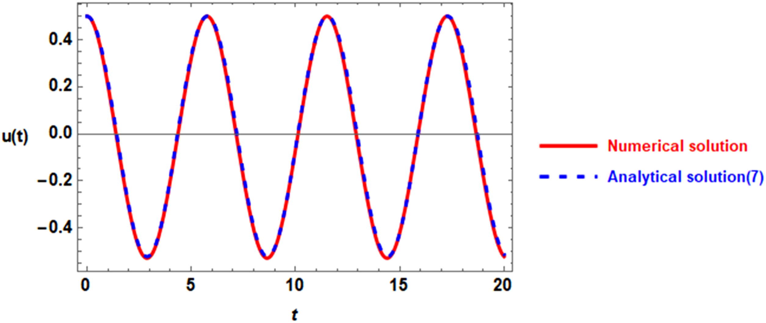
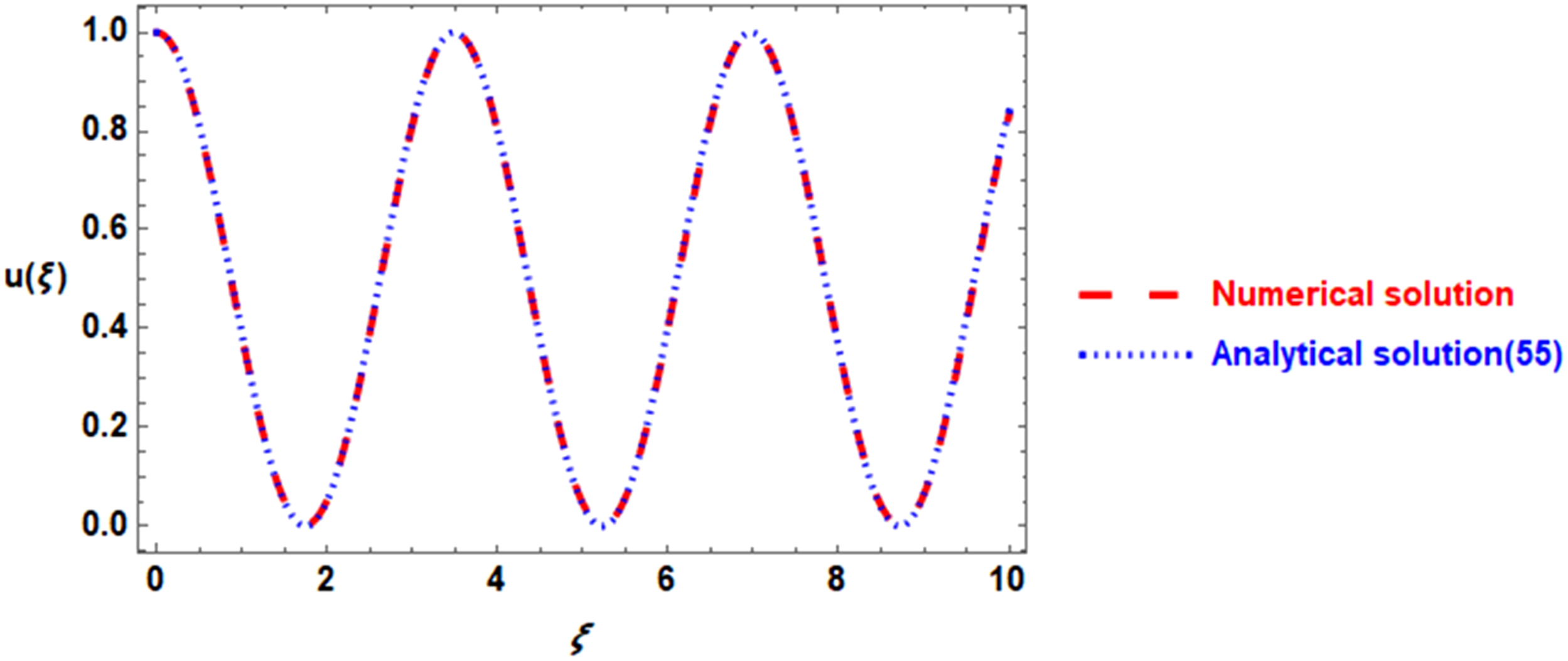
To demonstrate the accuracy maintained by the suggested approach, a numerical solution is useful for the examination. The comparison with the numerical solution of equation (3) is made to examine solution (7), and the calculations appear in Figure (1). The red-dash curve refers to the numerically exact solution of equation (3), while the blue-dot curve indicates the analytical solution (7). This comparison shows how the solution given by (5) and (6) is true (Table 1).

Table 1.

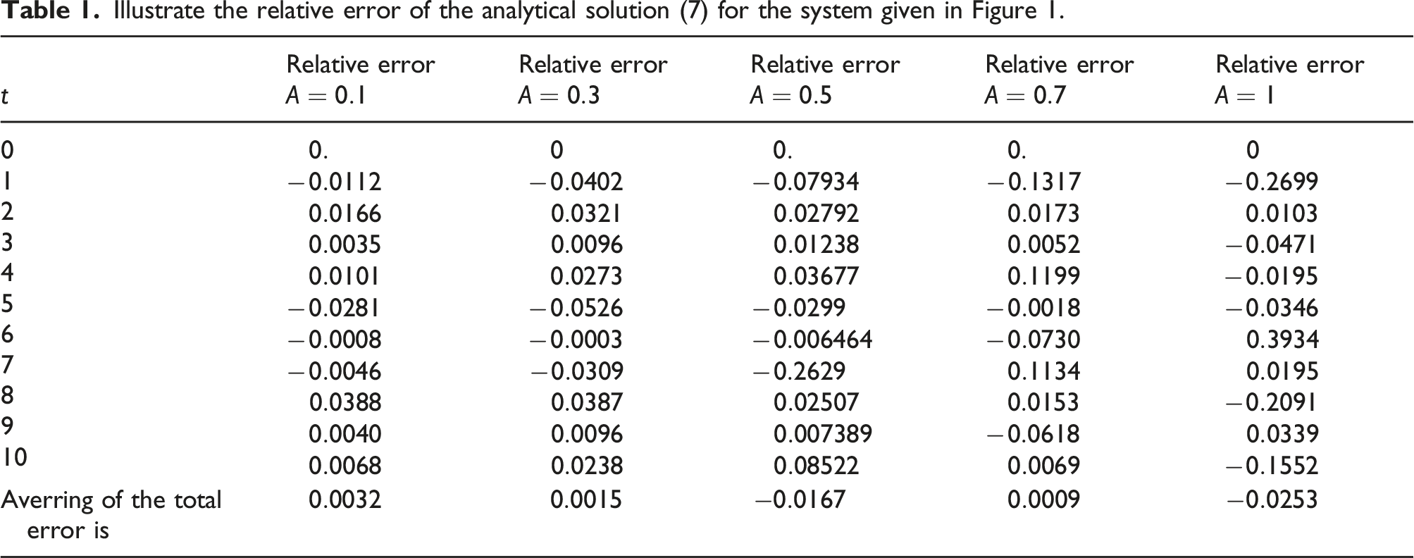
Illustrate the relative error of the analytical solution (7) for the system given in Figure 1.

$t$	Relative error $A=0.1$	Relative error $A=0.3$	Relative error $A=0.5$	Relative error $A=0.7$	Relative error $A=1$
0 1 2 3 4 5 6 7 8 9 10	$\begin{array}{c}0.\\ -0.0112\\ 0.0166\\ 0.0035\\ 0.0101\\ -0.0281\\ -0.0008\\ -0.0046\\ 0.0388 \\ 0.0040\\ 0.0068\end{array}$	$\begin{array}{c}0\\ -0.0402\\ 0.0321\\ 0.0096\\ 0.0273 \\ -0.0526 \\ -0.0003\\ -0.0309 \\ 0.0387\\ 0.0096\\ 0.0238\end{array}$	$\begin{array}{c}0.\\ -0.07934\\ 0.02792\\ 0.01238\\ 0.03677\\ -0.0299\\ -0.006464\\ -0.2629\\ 0.02507\\ 0.007389\\ 0.08522\end{array}$	$\begin{array}{c}0.\\ -0.1317\\ 0.0173 \\ 0.0052 \\ 0.1199\\ -0.0018 \\ -0.0730 \\ 0.1134\\ 0.0153 \\ -0.0618\\ 0.0069 \end{array}$	$\begin{array}{c}0\\ -0.2699\\ 0.0103 \\ -0.0471\\ -0.0195 \\ -0.0346\\ 0.3934\\ 0.0195\\ -0.2091\\ 0.0339\\ -0.1552\end{array}$
Averring of the total error is	$0.0032$	$0.0015$	$-0.0167$	$0.0009$	$-0.0253$

Figure 1.

Contrasting the analytical solution (7) (blue-dot curve) and the numerical solution of (3) (red-dash curve) for the system of $b_2=0.2,\hspace{0.17em}\hspace{0.17em}{a}_1=1,\hspace{0.17em}{a}_3=1\&A=\mathrm{0.5.}$

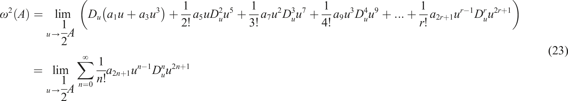
In the next sections, the aims are to investigate the frequency and the inhomogeneity due to extending the secular and non-secular parts of the restoring force to higher powers.

The strong Helmholtz–Duffing oscillator

In general, both the functions $f_{\mathit{odd}}\left(u\right)$ and $f_{\mathit{even}}\left(u\right)$ are defined as a polynomial in the odd and even powers, respectively

$$f_{\mathit{odd}}\left(u\right)=a_{1}u+a_3{u}^3+a_5{u}^5+\mathrm{...}{a}_{2n+1}{u}^{2n+1}={\displaystyle \sum _{n=0}^N{a}_{2n+1}{u}^{2n+1}}$$

(8)

$$f_{\mathit{even}}\left(u\right)=b_2{u}^2+b_4{u}^4+\mathrm{...}+b_{2n}{u}^{2n}={\displaystyle \sum _{n=1}^N{b}_{2n}{u}^{2n}}$$

(9)

Therefore, the general configuration of equation (1) becomes

$$\ddot{u}+{\displaystyle \sum _{n=0}^N{a}_{2n+1}{u}^{2n+1}}+{\displaystyle \sum _{n=1}^N{b}_{2n}{u}^{2n}}=0$$

(10)

If the coefficient $a_{2n+1}$ is replaced by $1/\left(2n+1\right)!$ and the coefficient $b_{2n}$ by $1/2n!$ into the nonlinear expansions, then (8) and (9) are reduced to

$$f_{\mathit{odd}}\left(u\right)={\displaystyle \sum _{n=0}^{\infty }\frac{u^{2n+1}}{\left(2n+1\right)!}}=\sinh u\hspace{1em}\text{and}$$

$$f_{\mathit{even}}\left(u\right)={\displaystyle \sum _{n=1}^{\infty }\frac{u^{2n}}{2n!}}=\cosh u-1={\displaystyle \underset{0}{\overset{u}{\int }}\sinh \left(x\right)dx=\cosh u-1}$$

Accordingly, equation (10) becomes

$$\ddot{u}\left(t\right)+e^{u\left(t\right)}-1=0$$

(11)

which is known as the Toda oscillator. ³⁴ This oscillator is a good example of the strong Helmholtz–Duffing oscillator. The equivalent of equation (11) is still given by the shape of (4), where ${\omega }^2\left(A\right)$ and $\sigma \left(A\right)$ are constants and have a modification covering the general case. Consequently, solution (7) is still satisfied in the general case. The use of He’s frequency formula (5) needs to be improved to cover the general case. It is only successful for the cubic Duffing equation. It is worthwhile to observe that both the frequency ${\omega }^2\left(A\right)$ and the non-secular part $\sigma \left(A\right)$ depend on each other, which is explained in what follows:

By integrating $f_{even}\left(u\right)$ for the variable $u$ , and letting $\frac{b_{2n}}{2n+1}$ be recalled by $a_{2n+1}$ , then the function $f_{\mathit{odd}}\left(u\right)-u$ will be found in the form of (8). In other words, by differentiating the function $f_{\mathit{odd}}\left(u\right)$ concerning the variable $u$ and letting $a_{2n+1}$ recall $b_{2n}/2n+1$ , the function $f_{\mathit{even}}\left(u\right)$ will be in the form of (9). Further, by integrating the function $f_{\mathit{odd}}\left(u\right)$ concerning the variable $u$ and letting $\frac{a_{2n+1}}{2n+2}$ recall $b_{2n+2}$ , the function $f_{\mathit{even}}\left(u\right)-b_0$ will be obtained.

The target is to show how to estimate the nonlinear frequency–amplitude relationship ${\omega }^2\left(A\right)$ and of the non-secular part $\sigma \left(A\right)$ , without using a perturbation technique.

Generalization formula for He’s frequency

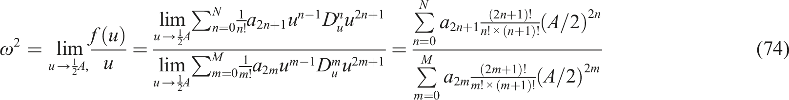
This section aims to show how to estimate the general form of He’s frequency formula to cover the family of the Duffing equation with nonlinearity having the higher powers. The procedure will be explained below:

If $n=0$ into equation (10), the linear harmonic equation is found, where its frequency can be estimated as

$${\omega }^2={\frac{f_{\mathit{odd}}\left(u\right)}{u}|}_{u=\frac{1}{2}A}=a_1$$

(12)

Making $n=1$ into expansion (8), the cubic Duffing’s equation arises where

$$f_{\mathit{odd}}\left(u\right)=a_{1}u+a_3{u}^3$$

(13)

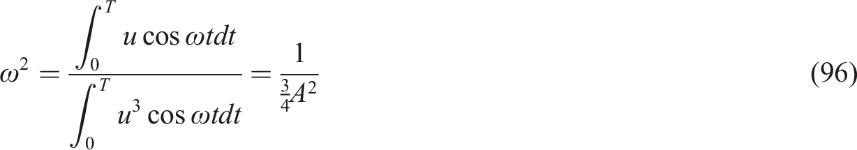
In this case, He ³³ has established the cubic Duffing’s frequency as equivalent to the first derivative of the function $f_{odd}\left(u\right)$ concerning the variable $u$ at the located point of $\overline{u}=\frac{1}{2}A.$

$${\omega }^2={\frac{d{f}_{\mathit{odd}}\left(u\right)}{du}|}_{u=\overline{u}=\frac{1}{2}A}=a_1+\frac{3}{4}{A}^2{a}_3$$

(14)

This frequency is in full agreement with that obtained by the perturbation methods; for example, see Ref. 35. Although He’s frequency–amplitude formulation is simple enough for practical applications, especially for the cubic Duffing oscillator, it is not the best for higher powers of the Duffing oscillator as shown in the following cases:

Using $n=2$ , the cubic–quintic Duffing equation arises where

$$f_{\mathit{odd}}\left(u\right)=a_{1}u+a_3{u}^3+a_5{u}^5$$

(15)

The estimation of the frequency to have ${\omega }^2$ the first derivative of the function $f\left(u\right)$ concerning the variable $u$ leads to

$${\omega }^2={\frac{d{f}_{\mathit{odd}}\left(u\right)}{du}|}_{u=\frac{1}{2}A}=a_1+\frac{3}{4}{A}^2{a}_3+\frac{5}{16}{A}^4{a}_5$$

(16)

This is exactly equivalent to that obtained by He, ³⁵ but it is not exactly equivalent to those obtained using the Modified Lindsted–Poincare solution. ¹⁴ In Ref. 36, the frequency–amplitude relationship is found to be

$${\omega }^2=a_1+\frac{3}{4}{A}^2{a}_3+\frac{5}{8}{A}^4{a}_5$$

(17)

Therefore, the use of the first-derivative $n>1$ does not guarantee the accuracy of the frequency obtained by a perturbation method. Investigating the above frequency shows that it can be read as

$${\omega }^2={\frac{d}{du}\left(a_{1}u+a_3{u}^3\right)+\frac{1}{2}\hspace{0.17em}{a}_{5}u\frac{d^2}{d{u}^2}\hspace{0.17em}{u}^5|}_{u=\frac{1}{2}A}$$

(18)

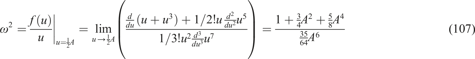
In addition, $n=3$ the septic power will be involved in the function $f\left(u\right)$ to become

$$f_{\mathit{odd}}\left(u\right)=a_{1}u+a_3{u}^3+a_5{u}^5+a_7{u}^7$$

(19)

Again, the estimation of frequency through the derivative $f_{odd}\left(u\right)$ concerning the variable $u$ at the location point $\frac{1}{2}A$ is

$${\omega }^2\left(A\right)={\frac{d{f}_{odd}\left(u\right)}{du}|}_{u=\frac{1}{2}A}=a_1+\frac{3}{4}{A}^2{a}_3+\frac{5}{16}{A}^4{a}_5+\frac{7}{64}\hspace{0.17em}{a}_7{A}^6$$

(20)

which does not agree with that obtained by HPM ¹⁴ and by the equivalent linearized method ³⁷

$${\omega }^2\left(A\right)=a_1+\frac{3}{4}{A}^2{a}_3+\frac{5}{8}{A}^4{a}_5+\frac{35}{64}{a}_7{A}^6$$

(21)

As mentioned before, the correct derivative approach is

$${\omega }^2\left(A\right)={\frac{d}{du}\left(a_{1}u+a_3{u}^3\right)+\frac{1}{2!}\hspace{0.17em}{a}_{5}u\frac{d^2}{d{u}^2}\hspace{0.17em}{u}^5+\frac{1}{3!}\hspace{0.17em}{a}_7{u}^2\frac{d^3}{d{u}^3}\hspace{0.17em}{u}^7|}_{u=\frac{1}{2}A}$$

(22)

For higher $n$ , the accurate derivative formula for estimating the frequency–amplitude relationship can be formulated as

$$\begin{array}{l}{\omega }^2\left(A\right)=\underset{u\to \frac{1}{2}A\hspace{0.17em}\hspace{0.17em}}{\lim }\left(D_u\left(a_{1}u+a_3{u}^3\right)+\frac{1}{2!}\hspace{0.17em}{a}_{5}u{D}_u^2{u}^5+\frac{1}{3!}\hspace{0.17em}{a}_7{u}^2{D}_u^3{u}^7+\frac{1}{4!}\hspace{0.17em}{a}_9{u}^3{D}_u^4{u}^9+\mathrm{...}+\frac{1}{r!}\hspace{0.17em}{a}_{2r+1}{u}^{r-1}{D}_u^r{u}^{2r+1}\right)\\ =\underset{u\to \frac{1}{2}A}{\lim }{\displaystyle \sum _{n=0}^{\infty }\frac{1}{n!}{a}_{2n+1}}{u}^{n-1}{D}_u^n{u}^{2n+1}\end{array}$$

(23)

which is the generation of He’s simplest frequency formula, which $D_u^n$ refers to the $n-$ order derivative concerning the variable $u$ The significance of this frequency may be seen by expanding the infinite series (23) which yields

$${\omega }^2\left(A\right)=a_1+\frac{3}{4}\hspace{0.17em}{a}_3{A}^2+\frac{5}{8}\hspace{0.17em}{a}_5{A}^4+\frac{35}{64}\hspace{0.17em}{a}_7{A}^6+\frac{63}{128}\hspace{0.17em}{a}_9{A}^8+\frac{231}{512}\hspace{0.17em}{a}_{11}{A}^{10}\mathrm{...}$$

(24)

This is the same as that obtained by Ref. 38. The above-mentioned series can be put in a power series form as

$$\begin{array}{l}{\omega }^2\left(A\right)=a_1+\frac{3!}{1!2!}\hspace{0.17em}{a}_3{\left(\frac{A}{2}\right)}^2+\frac{5!}{2!3!}\hspace{0.17em}{a}_5{\left(\frac{A}{2}\right)}^4+\frac{7!}{3!4!}\hspace{0.17em}{a}_7{\left(\frac{A}{2}\right)}^6+\frac{9!}{4!5!}\hspace{0.17em}{a}_9{\left(\frac{A}{2}\right)}^8+\frac{11!}{5!6!}\hspace{0.17em}{a}_{11}{\left(\frac{A}{2}\right)}^{10}+\mathrm{...}\\ ={\displaystyle \sum _{n=0}^{\infty }{a}_{2n+1}\frac{\left(2n+1\right)!}{n!\times \left(n+1\right)!}}{\left(\frac{A}{2}\right)}^{2n}\end{array}$$

(25)

This means that the frequency–amplitude relation has been sought in the style of the power series that is equivalent to the differentiative form (23).

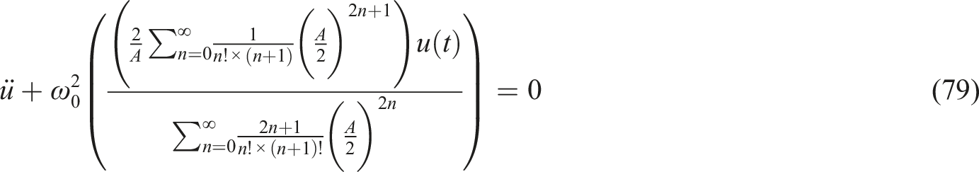
It is noted that if the coefficient $a_{2n+1}$ is replaced by ${\left(-1\right)}^n/\left(2n+1\right)!$ and the coefficient $b_{2n}$ by zero into the nonlinear equation (10), then it becomes in the following simple pendulum equation

$$\ddot{u}+\sin \hspace{0.17em}u=0$$

(26)

Its equivalent linearized form is derived using (25) to be

$$\ddot{u}+\frac{2}{A}{J}_1\left(A\right)u=0$$

(27)

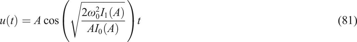
This means that the frequency of the simple pendulum motion is described as

$${\omega }^2\left(A\right)=\frac{2}{A}{J}_1\left(A\right)$$

(28)

This is the same as that obtained before in Ref. [14]. Its approximate solution can be performed in the form

$$u\left(t\right)=A\hspace{0.17em}\cos \sqrt{\frac{2}{A}{J}_1\left(A\right)}t$$

(29)

where $J_1\left(A\right)$ is the first kind of the Bessel functions of order one in the amplitude $A.$

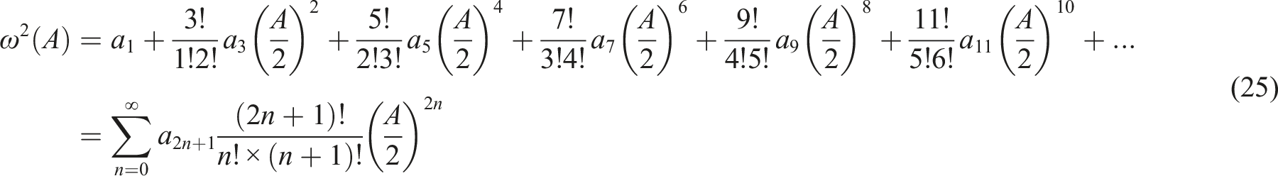
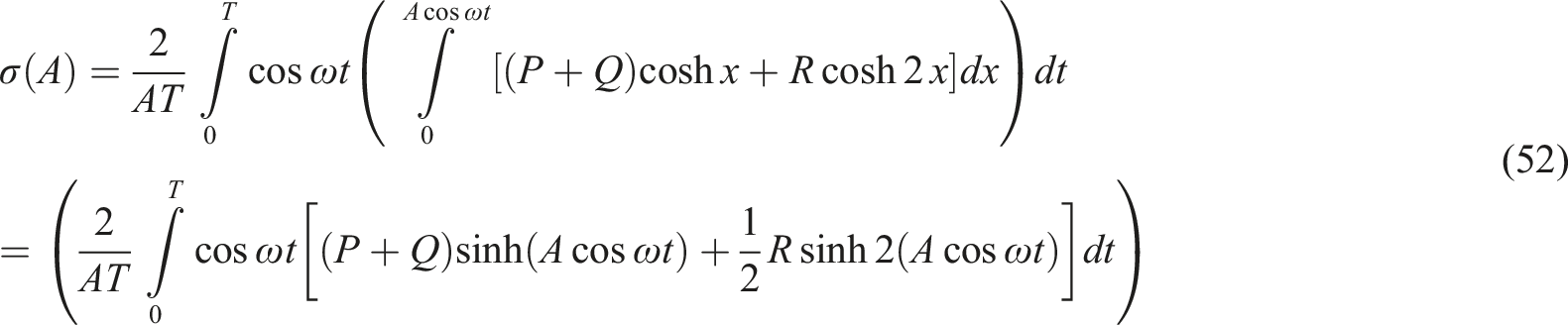
Generalization formula for the non-secular part

It is noted that when the non-secular part has the quadratic form, the inhomogeneity will come directly by replacing the displacement $u$ by $\frac{1}{2}A$ as shown in (6). This is true, only, up to the quadratic power, but for higher even powers, there is a requirement to establish an accurate immediate formula to estimate $\sigma \left(A\right)$ . Because the even function can be produced as a derivative of the odd function with replacing $a_{2n+1}$ to $\frac{b_{2n}}{2n+1}$ , then the non-secular parameter $\sigma \left(A\right)$ can be sought as

$$\sigma \left(A\right)={f_{\mathit{even}}\left(u\right)|}_{u=\frac{1}{2}A}={\frac{d}{du}{f}_{\mathit{odd}}\left(u\right)|}_{\begin{array}{l}u=\frac{1}{2}A\\ a_{2n+1}\to \frac{b_{2n}}{2n+1}\end{array}}={{\omega }^2\left(A\right)|}_{a_{2n+1}\to \frac{b_{2n}}{2n+1}}={\displaystyle \sum _{n=1}^{\infty }{b}_{2n}\frac{2n!}{n!\times \left(n+1\right)!}}{\left(\frac{A}{2}\right)}^{2n}$$

(30)

This is the equivalent of the non-secular term which appears as the inhomogeneous part of the equivalent equation of the nonlinear oscillator. Expanding the above expansion, the formula for the non-secular $\sigma \left(A\right)$ will be

$$\sigma \left(A\right)={\displaystyle \sum _{n=1}^N{b}_{2n}\frac{2n!}{n!\times \left(n+1\right)!}}{\left(\frac{A}{2}\right)}^{2n}=\frac{1}{4}{b}_2{A}^2+\frac{1}{8}{b}_4{A}^4+\frac{5}{64}{b}_6{A}^6+\frac{7}{128}{b}_8{A}^8+\mathrm{...}$$

(31)

It is noted that the equivalent differentiative form of the non-secular part $\sigma \left(A\right)$ can be performed as

$$\sigma \left(A\right)=\underset{u\to \frac{1}{2}A}{\lim }{\displaystyle \sum _{m=1}^M\frac{1}{\left(m+1\right)!}{b}_{2m}}{u}^m{D}_u^m{u}^{2m}$$

(32)

where $M$ is a general integer number. This formula is derived for the first time.

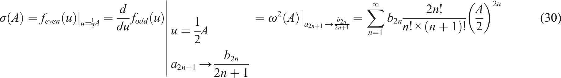
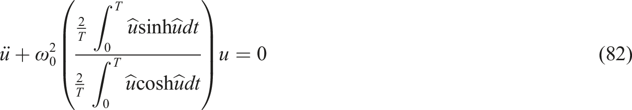
Performance of the frequency formula in the integrative form

The best derivation of the frequency formula comes through using the weighted residuals technology. The use of He’s formalism is useful to compute the frequency for the higher $n$ the generalized $f_{odd}\left(u\right)$ . The frequency can be computed approximately by applying the weighted residuals that were approached by Ref [39].

Based on the formula of

$$\frac{2}{\pi }{\displaystyle \underset{0}{\overset{\pi /2}{\int }}{\cos }^{2m}\xi d\xi }=\frac{2m-1}{2m}$$

(33)

the power series (24) can be rearranged and sought in the integrative configuration as

$${\omega }^2\left(A\right)=\frac{2}{A^{2}T}{a}_1{\displaystyle \underset{0}{\overset{T}{\int }}{\widehat{u}}^{2}dt}+a_3\frac{2}{A^{2}T}{\displaystyle \underset{0}{\overset{T}{\int }}{\widehat{u}}^{4}dt}+a_5\frac{2}{A^{2}T}{\displaystyle \underset{0}{\overset{T}{\int }}{\widehat{u}}^{6}dt}+a_7\frac{2}{A^{2}T}{\displaystyle \underset{0}{\overset{T}{\int }}{\widehat{u}}^{6}dt}+\mathrm{...}$$

$$\begin{array}{l}{\omega }^2\left(A\right)=\frac{2}{A^2}{\displaystyle \sum _{n=0}^N{a}_{2n+1}}\frac{1}{T}{\displaystyle \underset{0}{\overset{T}{\int }}{\widehat{u}}^{2n+2}dt}=\frac{2}{A^{2}T}{\displaystyle \underset{0}{\overset{T}{\int }}{\displaystyle \sum _{n=0}^N{a}_{2n+1}}{\widehat{u}}^{2n+2}dt}\\ =\frac{2}{A^{2}T}{\displaystyle \underset{0}{\overset{T}{\int }}}\widehat{u}{f}_{\mathit{odd}}\left(\widehat{u}\right)dt=\frac{1}{2{\overline{u}}^{2}T}{\displaystyle \underset{0}{\overset{T}{\int }}}\widehat{u}{f}_{odd}\left(\widehat{u}\right)dt;\hspace{1em}T=\frac{\pi }{2\omega }\end{array}$$

(34)

where $\widehat{u}=A\cos \omega t$ is the trial solution of the generalized oscillator (10). The term ${\overline{u}}^2$ refers to the least mean square displacement.^27,28

To perform the integrative shape of the Helmholtz parameter $\sigma \left(A\right)$ , the function $f_{\mathit{odd}}\left(\widehat{u}\right)$ in (34) will be replaced $\left({\displaystyle \underset{0}{\overset{u\left(t\right)}{\int }}{f}_{\mathit{even}}\left(x\right)dx}\right)$ to become

$$\sigma \left(A\right)=\frac{1}{2{\overline{u}}^{2}T}{\displaystyle \underset{0}{\overset{T}{\int }}\widehat{u}\left(t\right)\left({\displaystyle \underset{0}{\overset{\widehat{u}\left(t\right)}{\int }}{f}_{\mathit{even}}\left(x\right)dx}\right)}dt=b_0+\frac{1}{4}{b}_2{A}^2+\frac{1}{8}{b}_4{A}^4+\frac{5}{64}{b}_6{A}^6+\frac{7}{128}{b}_8{A}^8+\dots$$

(35)

It is noted that the above expansion coincides with the results obtained in (31) or (32). To this end, Helmholtz–Duffing oscillator equation (4) can be sought in the following integrative configuration

$$\ddot{u}\left(t\right)+\left(\frac{1}{T}{\displaystyle \underset{0}{\overset{T}{\int }}\left({\partial }_A\widehat{u}\right)\frac{f_{\mathit{odd}}\left(\widehat{u}\right)}{\overline{u}}dt}\right)u\left(t\right)+\frac{1}{T}{\displaystyle \underset{0}{\overset{T}{\int }}\left({\partial }_A\widehat{u}\right)\left({\displaystyle \underset{0}{\overset{\widehat{u}\left(t\right)}{\int }}\frac{f_{\mathit{even}}\left(x\right)}{\overline{u}}dx}\right)}dt=0$$

(36)

Some application to strong nonlinearity

In this section, the generalization frequency approach is applied to two examples of strong nonlinearity for illustration.

The application to the Toda oscillator

This section is devoted to briefly describing the following Toda oscillator^40,41

$$\ddot{u}+e^u-1=0;\hspace{1em}u\left(0\right)=A\&\dot{u}\left(0\right)=0$$

(37)

It is worthwhile to observe that the use of the function $f\left(u\right)=e^u-1$ to estimate the frequency of equation (36), directly, is not suitable because it is composed of the odd and the even nonlinearity forces together. It is better to separate nonlinearity into secular and non-secular functions. Replacing the exponential function in equation (37) with its equivalent of the hyperbolic functions $\cosh \hspace{0.17em}u$ and $\sinh \hspace{0.17em}u$ yields

$$\ddot{u}+\sinh u=1-\cosh u$$

(38)

Selecting

$$f_{\mathit{odd}}\left(u\right)=\sinh u\hspace{1em}\text{and}\hspace{1em}{f}_{\mathit{even}}\left(u\right)=\text{cosh }u-1$$

(39)

At this stage, the solution of the Toda oscillator will be obtained by using the power series forms (25) and (31) or by applying the technology of the weighted residuals formats (34) and (35).

In the first approach, it is required to use the power series forms of $\sinh u$ and $\text{cosh }u$ . Therefore, the coefficient $a_{2n+1}$ can be replaced by $1/\left(2n+1\right)!$ and the coefficient $b_{2n}$ by $1/2n!$ into the expansions (25) and (31), and accordingly the Toda oscillator will have the form

$$\ddot{u}\left(t\right)+\left({\displaystyle \sum _{n=0}^{\infty }\frac{1}{n!\times \left(n+1\right)!}}{\left(\frac{A}{2}\right)}^{2n}\right)u\left(t\right)+{\displaystyle \sum _{n=0}^{\infty }\frac{1}{n!\times \left(n+1\right)!}}{\left(\frac{A}{2}\right)}^{2n}-1=0$$

(40)

According to the definition of the modified Bessel function, equation (40) becomes

$$\ddot{u}\left(t\right)+\frac{2}{A}{I}_1\left(A\right)u\left(t\right)+\frac{2}{A}{I}_1\left(A\right)-1=0$$

(41)

This is the equivalent form of the Toda oscillator equation (37), which has the following solution

$$u\left(t\right)=\left(A-\frac{A-2I_1\left(A\right)}{2I_1\left(A\right)}\right)\cos \sqrt{\frac{2}{A}{I}_1\left(A\right)}t+\frac{A-2I_1\left(A\right)}{2I_1\left(A\right)}$$

(42)

where $I_1\left(A\right)$ is the modified Bessel function of the first kind in $A$ .

To obtain the solution of the Toda oscillator equation (37) using the weighted residuals technology, the secular function $f_{\mathit{odd}}\left(\widehat{u}\right)$ and the non-secular function $f_{even}\left(\widehat{u}\right)$ are selected as the forms given in (39). Employing these functions in (34) and (35) and applying the integral form of the first kind of the Bessel functions which is defined as

$$\frac{1}{\pi }{\displaystyle \underset{0}{\overset{\pi }{\int }}\cos \hspace{0.17em}t\hspace{0.17em}\sinh \left(x\hspace{0.17em}\cos t\right)dt}=I_1\left(x\right)$$

(43)

the frequency ${\omega }^2\left(A\right)$ and the inhomogeneity term $\sigma \left(A\right)$ come in the form

$${\omega }^2\left(A\right)=\frac{1}{2{\overline{u}}^{2}T}{\displaystyle \underset{0}{\overset{T}{\int }}\widehat{u}\hspace{0.17em}\sinh \left(\widehat{u}\right)dt}=\frac{2}{\hspace{0.17em}AT}{\displaystyle \underset{0}{\overset{T}{\int }}\left(\cos \omega t\right)\sinh \left(\cos \hspace{0.17em}\omega t\right)dt}=\frac{2}{A}{I}_1\left(A\right)$$

(44)

$$\sigma \left(A\right)=\frac{1}{2{\overline{u}}^{2}T}{\displaystyle \underset{0}{\overset{T}{\int }}\widehat{u}\left(t\right)\left({\displaystyle \underset{0}{\overset{\widehat{u}\left(t\right)}{\int }}\left(\cosh x-1\right)dx}\right)}dt=\frac{2}{A^{2}T}{\displaystyle \underset{0}{\overset{T}{\int }}\widehat{u}\left(\sinh \left(\widehat{u}\right)-\widehat{u}\right)dt}=\frac{2}{A}{I}_1\left(A\right)-1$$

(45)

Accordingly, the solution of the Toda oscillator has the form of (42).

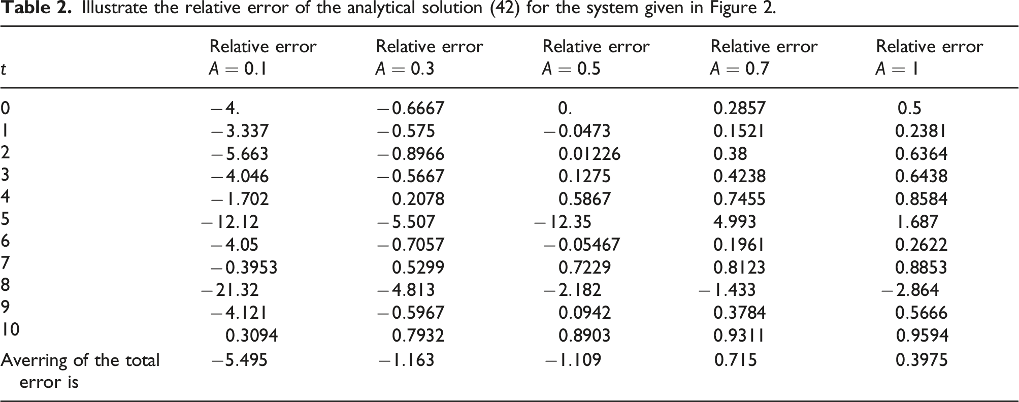
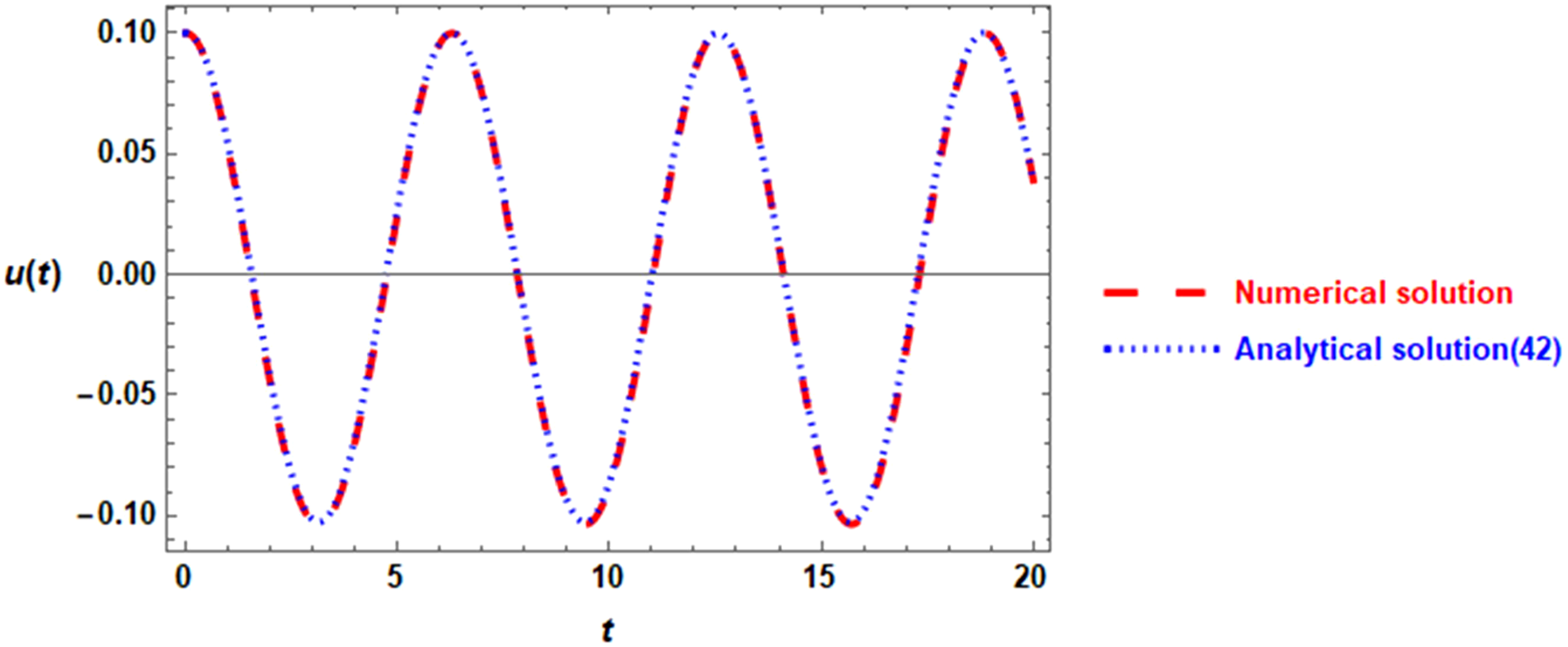
The numerical illustration of Toda’s frequency formula is displayed in Figure (2). The comparison with the numerical solution shows that the analytic periodic solution (42) (blue-dot curve) has a good agreement with the numerical solution (red-dash curve) (Table 2).

Table 2.

Illustrate the relative error of the analytical solution (42) for the system given in Figure 2.

$t$	Relative error $A=0.1$	Relative error $A=0.3$	Relative error $A=0.5$	Relative error $A=0.7$	Relative error $A=1$
0 1 2 3 4 5 6 7 8 9 10	$\begin{array}{c}-4.\\ -3.337\\ -5.663\\ -4.046\\ -1.702\\ -12.12\\ -4.05\\ -0.3953\\ -21.32\\ -4.121\\ 0.3094\end{array}$	$\begin{array}{c}-0.6667\\ -0.575\\ -0.8966\\ -0.5667\\ 0.2078\\ -5.507\\ -0.7057\\ 0.5299\\ -4.813\\ -0.5967\\ 0.7932\end{array}$	$\begin{array}{c}0.\\ -0.0473\\ 0.01226\\ 0.1275\\ 0.5867\\ -12.35\\ -0.05467\\ 0.7229\\ -2.182\\ 0.0942\\ 0.8903\end{array}$	$\begin{array}{c}0.2857\\ 0.1521\\ 0.38\\ 0.4238\\ 0.7455\\ 4.993\\ 0.1961\\ 0.8123\\ -1.433\\ 0.3784\\ 0.9311\end{array}$	$\begin{array}{c}0.5\\ 0.2381\\ 0.6364\\ 0.6438\\ 0.8584\\ 1.687\\ 0.2622\\ 0.8853\\ -2.864\\ 0.5666\\ 0.9594\end{array}$
Averring of the total error is	$-5.495$	$-1.163$	$-1.109$	$0.715$	$0.3975$

Figure 2.

Contrasting between the numerical solution of equation (37) (red-dash curve) and the analytical solution (42) (blue-dot curve), for a system having the amplitude $A=0.1$ .

The application to Zhiber–Shabat oscillator

This section aims to give another application to our proposal. The Zhiber–Shabat (ZS) equation is a partial differential equation having three kinds of exponential nonlinear terms.^42,43 This equation is derived in the form

$$u_{xt}+p{e}^u+q{e}^{-u}+r{e}^{-2u}=0;\hspace{1em}u=u\left(x,t\right)$$

(46)

where $p,\hspace{0.17em}q$ and $r$ are physical constants. Under the traveling wave transformation, equation (46) becomes

$$u^{″}+P{e}^u+Q{e}^{-u}+{\mathrm{Re}}^{-2u}=0;\hspace{1em}u=u\left(\xi \right)$$

(47)

where the new variable $\xi$ is defined by

$$\xi \left(x,t\right)=x-ct;\hspace{1em}c\ne 0$$

(48)

The constant $c$ refers to the wave velocity, and the coefficients in equation (46) are

$P=-1/cp,\hspace{0.17em}Q=-1/cq$ and $R=-1/cr$

Suppose that equation (47) is subject to the initial conditions $u\left(0\right)=A$ and $u^{\prime }\left(0\right)=0$ . This equation can be converted to the hyperbolic functions $\cosh \hspace{0.17em}u$ and $\sinh \hspace{0.17em}u$ in the following form

$$u^{″}+f_{\mathit{odd}}\left(u\right)+f_{\mathit{even}}\left(u\right)=0$$

(49)

where the even and the odd functions are described in the form

$$\begin{array}{l}{f}_{\mathit{odd}}\left(u\right)=\left(P-Q\right)\sinh u-R\sinh 2u\\ f_{\mathit{even}}\left(u\right)=\left(P+Q\right)\cosh u+R\cosh 2u\end{array}$$

(50)

As seen, the Zhiber–Shabat equation (47) represents a model of the Helmholtz–Duffing oscillator. It is noted that the solution of (49) has the form of (7). To perform the frequency ${\omega }^2\left(A\right)$ and the inhomogeneity part $\sigma \left(A\right)$ , the integral form given by (34) and (35) is used, where the trial solution of equation (49) may be introduced as $\widehat{u}=A\cos \omega t$ . Thus, by Employing the definition (50) with the expansion of the integral forms given by (34) and (35), the results are reduced to

$${\omega }^2\left(A\right)=\left(\frac{2}{AT}{\displaystyle \underset{0}{\overset{T}{\int }}\cos \omega t\left[\left(P-Q\right)\sinh \left(A\hspace{0.17em}\cos \hspace{0.17em}\omega t\right)-R\sinh 2\left(A\hspace{0.17em}\cos \hspace{0.17em}\omega t\right)\right]}dt\right)$$

(51)

$$\begin{array}{l}\sigma \left(A\right)=\frac{2}{AT}{\displaystyle \underset{0}{\overset{T}{\int }}\cos \omega t\left({\displaystyle \underset{0}{\overset{A\hspace{0.17em}\cos \hspace{0.17em}\omega t}{\int }}\left[\left(P+Q\right)\cosh x+R\cosh 2x\right]dx}\right)}dt\\ =\left(\frac{2}{AT}{\displaystyle \underset{0}{\overset{T}{\int }}\cos \hspace{0.17em}\omega t\left[\left(P+Q\right)\sinh \left(A\hspace{0.17em}\cos \hspace{0.17em}\omega t\right)+\frac{1}{2}R\sinh 2\left(A\hspace{0.17em}\cos \hspace{0.17em}\omega t\right)\right]dt}\right)\end{array}$$

(52)

Using the formula (43) yields

$${\omega }^2\left(A\right)=\frac{2}{A}\left(P-Q\right)I_1\left(A\right)-\frac{2}{A}R{I}_1\left(2A\right)$$

(53)

$$\sigma \left(A\right)=\frac{2}{A}\left(P+Q\right)I_1\left(A\right)+\frac{1}{A}R{I}_1\left(2A\right)$$

(54)

Employing (53) and (54) into the form of the solution given by (7), the solution of equation (49) will be performed as

$$u\left(\xi \right)=\left(A+\frac{\sigma }{{\omega }^2}\right)\cos \hspace{0.17em}\omega \xi -\frac{\sigma }{{\omega }^2}$$

(55)

It is noted that the periodic solution (54) requires that

$$\left(P-Q\right)I_1\left(A\right)-R{I}_1\left(2A\right)>0$$

(56)

If $P=Q$ , then the coefficient $R$ must have a negative value to satisfy the above condition for the periodic solution. Since $I_1\left(A\right)<I_1\left(2A\right)$ , then the negative values for the coefficient $Q$ require that the coefficient $R$ must be small enough in such a way that

$$R<\left(P-Q\right)\frac{I_1\left(A\right)}{I_1\left(2A\right)}$$

(57)

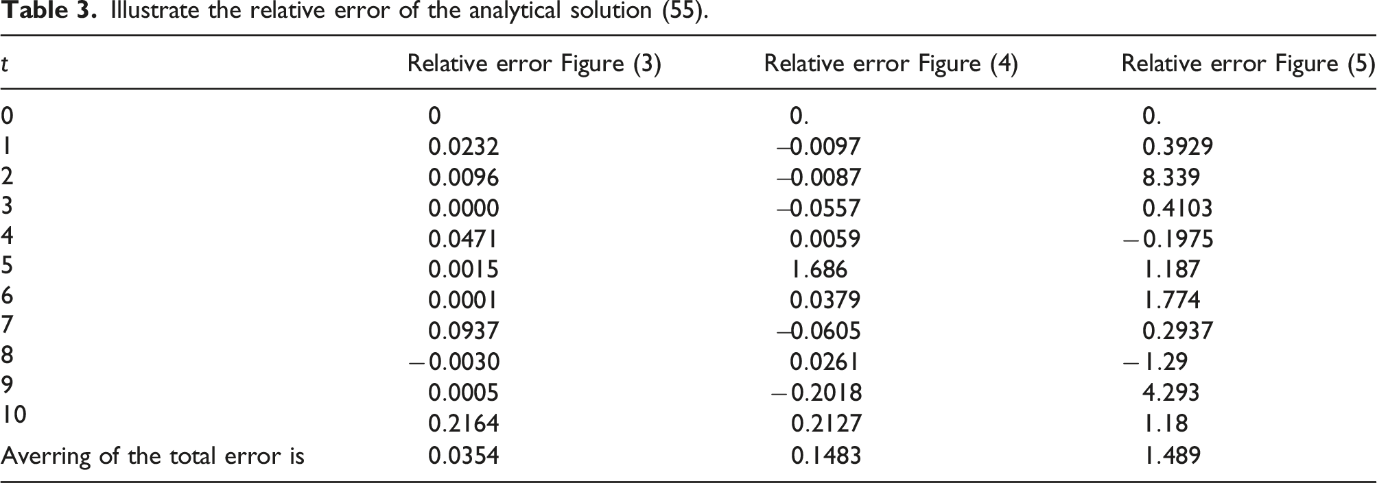
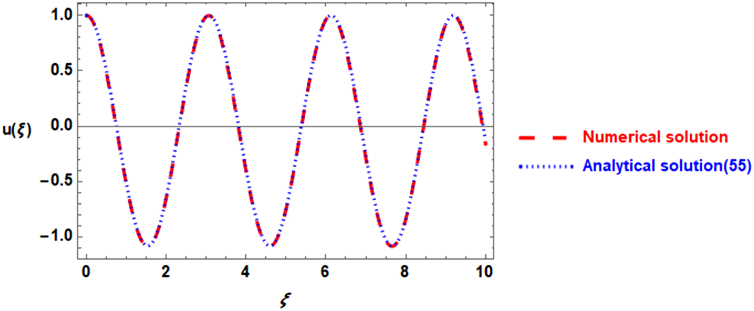
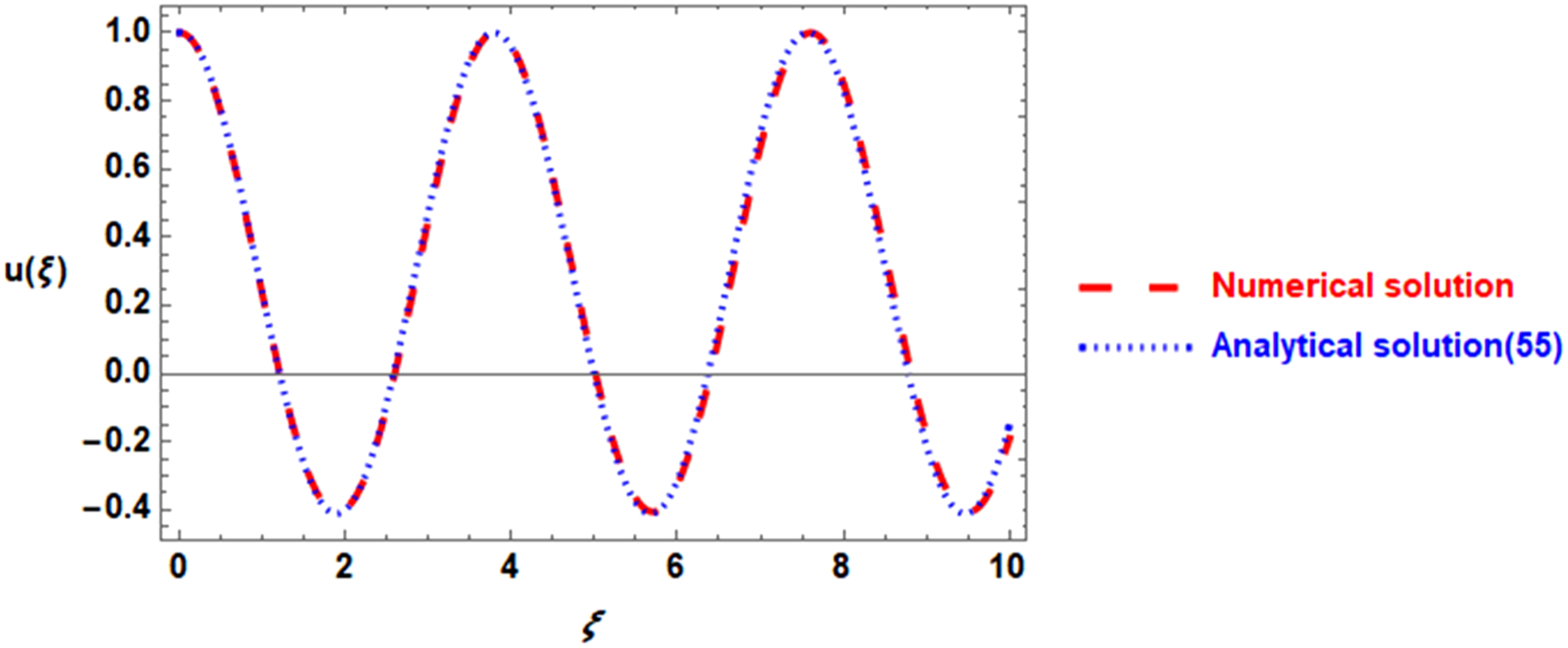
The original equation (47) was solved numerically by Mathematica software and was compared with the obtained solution (55). The examination of the originality of the fast simple solution is proposed in this work. This comparison appears in Figure (3). The system for calculation is selected as $P=2,\hspace{0.17em}Q=-2,\hspace{0.17em}R=0.1$ , and $A=1$ . Another example $P=1,\hspace{0.17em}Q=-2,\hspace{0.17em}R=0.2$ is used to plot in Figure (4). The same system with an increase in the parameter $R$ to become $R=0.4$ has been plotted in Figure (5). The investigation of these graphs shows the presence of low error, which will decrease as the amplitude $A$ increases (Table 3).

Table 3.

Illustrate the relative error of the analytical solution (55).

$t$	Relative error Figure (3)	Relative error Figure (4)	Relative error Figure (5)
0 1 2 3 4 5 6 7 8 9 10	$\begin{array}{c}0\\ 0.0232\\ 0.0096\\ 0.0000\\ 0.0471\\ 0.0015\\ 0.0001\\ 0.0937\\ -0.0030 \\ 0.0005\\ 0.2164\end{array}$	$\begin{array}{c}0.\\ \mathrm{-}0.0097 \\ \mathrm{-}0.0087\\ \mathrm{-}0.0557 \\ 0.0059 \\ 1.686\\ 0.0379 \\ \mathrm{-}0.0605\\ 0.0261\\ -0.2018\\ 0.2127\end{array}$	$\begin{array}{c}0.\\ 0.3929\\ 8.339\\ 0.4103\\ -0.1975\\ 1.187\\ 1.774\\ 0.2937\\ -1.29\\ 4.293\\ 1.18\end{array}$
Averring of the total error is	$0.0354$	$0.1483$	$1.489$

Table 4.

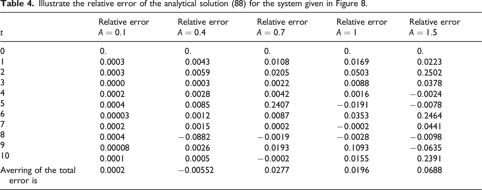
Illustrate the relative error of the analytical solution (88) for the system given in Figure 8.

$t$	Relative error $A=0.1$	Relative error $A=0.4$	Relative error $A=0.7$	Relative error $A=1$	Relative error $A=1.5$
0 1 2 3 4 5 6 7 8 9 10	$\begin{array}{c}0.\\ 0.0003\\ 0.0003\\ 0.0000\\ 0.0002\\ 0.0004\\ 0.00003 \\ 0.0002\\ 0.0004\\ 0.00008\\ 0.0001\end{array}$	$\begin{array}{c}0.\\ 0.0043\\ 0.0059\\ 0.0003\\ 0.0028\\ 0.0085\\ 0.0012\\ 0.0015\\ -0.0882\\ 0.0026\\ 0.0005 \end{array}$	$\begin{array}{c}0.\\ 0.0108\\ 0.0205\\ 0.0022\\ 0.0042\\ 0.2407\\ 0.0087\\ 0.0002\\ -0.0019\\ 0.0193\\ -0.0002\end{array}$	$\begin{array}{c}0.\\ 0.0169\\ 0.0503\\ 0.0088\\ 0.0016\\ -0.0191\\ 0.0353\\ -0.0002\\ -0.0028\\ 0.1093\\ 0.0155\end{array}$	$\begin{array}{c}0.\\ 0.0223\\ 0.2502\\ 0.0378\\ -0.0024\\ -0.0078\\ 0.2464\\ 0.0441\\ -0.0098\\ -0.0635\\ 0.2391\end{array}$
Averring of the total error is	$0.0002$	$-0.00552$	$0.0277$	$0.0196$	$0.0688$

Figure 3.

Contrasting between the numerical solution of equation (47) (red-dash curve) and the analytical solution (55) (blue-dot curve), for a system having the amplitude $A=1$ with the coefficients $P=2,\hspace{0.17em}Q=-2,\hspace{0.17em}R=.1$ .

Figure 4.

Contrasting between the numerical solution of equation (47) (red-dash curve) and the analytical solution (55) (blue-dot curve), for a system having the amplitude $A=1$ with the coefficients $P=1,\hspace{0.17em}Q=-2,\hspace{0.17em}R=.2$ .

Figure 5.

Contrasting between the numerical solution of equation (47) (red-dash curve) and the analytical solution (55) (blue-dot curve), for a system having the amplitude $A=1$ with the coefficients $P=1,\hspace{0.17em}Q=-3,\hspace{0.17em}R=0.4$ .

Oscillators with a relative restoring force

This section focuses on oscillators with an even denominator of the odd restoring force. A variety of restoring forces with an even denominator has been obtained in the literature. Herein, three examples will be discussed: the tangent oscillator ^44,45, cubic and cubic–quintic oscillators having mixture of the displacement, velocity, and acceleration variables.^46,47

Application to vibration mode of a tapered beam

The differential equation corresponding to the fundamental vibration mode of a tapered beam ⁴⁶ is described as

$$\ddot{u}+u+\alpha u^3+\beta \left(u^2\ddot{u}+u{\dot{u}}^2\right)=0$$

(58)

where u is displacement, $\alpha$ and $\beta$ are arbitrary constants. Subject to the following initial conditions

$$u\left(0\right)=A,\hspace{1em}\dot{u}\left(0\right)=0$$

(59)

This oscillator can be rearranged as

$$\ddot{u}+f\left(u\right)=0$$

(60)

where the restoring force $f\left(u\right)$ is given by

$$f\left(u\right)=\frac{u+\alpha u^3+\beta u{\dot{u}}^2}{1+\beta u^2}$$

(61)

Due to the odd functional, the frequency is estimated as

$${\omega }^2=\underset{\begin{array}{l}u\to \frac{1}{2}A,\\ \dot{u}\to \frac{1}{2}A\omega \end{array}}{\lim }\frac{f\left(u\right)}{u}=\underset{\begin{array}{l}u\to \frac{1}{2}A,\\ \dot{u}\to \frac{1}{2}A\omega \end{array}}{\lim }\frac{\frac{d}{du}\left(u+\alpha u^3+\beta u{\dot{u}}^2\right)}{\frac{d}{du}\left(u+\beta u^3\right)}=\frac{1+3/4A^2\alpha +1/4A^2\beta {\omega }^2}{1+3/4A^2\beta }$$

(62)

Consequently, the frequency is performed in the form

$${\omega }^2=\frac{1+3/4A^2\alpha }{1+1/2A^2\beta }$$

(63)

The application of Galerkin’s method with the trial solution $A\cos \omega t$ leads to the same frequency formula as follows

$$\frac{2}{A^{2}T}{\displaystyle {\int }_0^T\left(\ddot{u}\left(1+\beta u^2\right)+u+\alpha u^3+\beta u{\dot{u}}^2\right)\cos \hspace{0.17em}\omega tdt}=1+\frac{3}{4}{A}^2\alpha -{\omega }^2\left(1+\frac{1}{2}{A}^2\beta \right)=0$$

(64)

The approximate solution of equation (57) becomes

$$u\left(t\right)=A\cos \hspace{0.17em}\omega t$$

(65)

The free vibrations of a conservative oscillator with type fifth-order nonlinearities [47] is expressed by

$$\ddot{x}+{\omega }_0^{2}x+a_1{x}^3+a_2\left(x^2\ddot{x}+x{\dot{x}}^2\right)+b_1{x}^5+b_2\left(x^4\ddot{x}+2x^3{\dot{x}}^2\right)=0$$

(66)

with the initial conditions: $x\left(0\right)=A,\hspace{0.17em}\dot{x}\left(0\right)=0.$ Rewrite the above equation in the form

$$\ddot{x}\left(1+a_2{x}^2+b_2{x}^4\right)+\left({\omega }_0^{2}x+a_1{x}^3+b_1{x}^5\right)+\left(a_{2}x+2b_2{x}^3\right){\dot{x}}^2=0$$

(67)

Accordingly, the restoring force $f\left(x\right)$ can be written as

$$f\left(x\right)=\frac{\left({\omega }_0^{2}x+a_1{x}^3+b_1{x}^5\right)+\left(a_{2}x+2b_2{x}^3\right){\dot{x}}^2}{1+a_2{x}^2+b_2{x}^4}$$

(68)

Thus, the frequency is evaluated as

$$\begin{array}{l}{\omega }^2=\underset{\begin{array}{l}x\to \frac{1}{2}A,\\ \dot{x}\to \frac{1}{2}A\omega \end{array}}{\lim }\frac{f\left(x\right)}{x}=\underset{\begin{array}{l}x\to \frac{1}{2}A,\\ \dot{x}\to \frac{1}{2}A\omega \end{array}}{\lim }\left(\frac{D_x\left({\omega }_0^{2}x+a_1{x}^3\right)+1/2!x{D}_x^2{b}_1{x}^5+{\dot{x}}^2{D}_x\left(a_{2}x+2b_2{x}^3\right)}{D_x\left(x+a_2{x}^3\right)+1/2!x{D}_x^2{b}_2{x}^5}\right)\\ =\frac{{\omega }_0^2+3/4A^2{a}_1+5/8A^4{b}_1+1/4A^2{\omega }^2\left(a_2+3/2b_2{A}^2\right)}{1+3/4A^2{a}_2+5/8A^4{b}_2}\end{array}$$

(69)

After simplification, the frequency is found to be

$${\omega }^2=\frac{{\omega }_0^2+3/4A^2{a}_1+5/8A^4{b}_1}{\left(1+1/2A^2{a}_2+2/8A^4{b}_2\right)}$$

(70)

By choosing the trial solution as mentioned before, the frequency due to the Galerkin method has the form

$$\frac{2}{A^{2}T}{\displaystyle {\int }_0^T\left(\ddot{x}\left(1+a_2{x}^2+b_2{x}^4\right)+\left({\omega }_0^{2}x+a_1{x}^3+b_1{x}^5\right)+\left(a_{2}x+2b_2{x}^3\right){\dot{x}}^2\right)\cos \hspace{0.17em}\omega tdt}=0$$

(71)

which yields

$${\omega }^2=\frac{{\omega }_0^2+3/4A^2{a}_1+5/8A^4{b}_1}{\left(1+1/2A^2{a}_2+3/8A^4{b}_2\right)}$$

(72)

Remark:

In general, when the restoring force of the oscillator is composed of an odd polynomial function in the numerator and even polynomial function in the denominator such as

$$f\left(u\right)=\frac{{\displaystyle \sum _{n=0}^N{a}_{2n+1}{u}^{2n+1}}}{{\displaystyle \sum _{m=0}^N{a}_{2n}{u}^{2m}}}$$

(73)

The frequency $\omega$ will be estimated to be

$${\omega }^2=\underset{u\to \frac{1}{2}A,}{\lim }\frac{f\left(u\right)}{u}=\frac{\underset{u\to \frac{1}{2}A}{\lim }{\displaystyle {\sum }_{n=0}^N\frac{1}{n!}{a}_{2n+1}}{u}^{n-1}{D}_u^n{u}^{2n+1}}{\underset{u\to \frac{1}{2}A}{\lim }{\displaystyle {\sum }_{m=0}^M\frac{1}{m!}{a}_{2m}}{u}^{m-1}{D}_u^m{u}^{2m+1}}=\frac{{\displaystyle \sum _{n=0}^N{a}_{2n+1}\frac{\left(2n+1\right)!}{n!\times \left(n+1\right)!}}{\left(A/2\right)}^{2n}}{{\displaystyle \sum _{m=0}^M{a}_{2m}\frac{\left(2m+1\right)!}{m!\times \left(m+1\right)!}}{\left(A/2\right)}^{2m}}$$

(74)

where $N$ and $M$ are integer numbers.

Application to the Tangent Oscillator

The tangent oscillator is found in the form^44–45

$$\ddot{u}+{\omega }_0^2\tan \hspace{0.17em}u=0;\hspace{1em}u\left(0\right)=A,\hspace{1em}\dot{u}\left(0\right)=0$$

(75)

Since the frequency formula of the nonlinear oscillator can be derived by two approaches, He’s frequency formula and the weighted residuals technology; these two methods should lead to the same results. In Ref. 45, He’s frequency formula is applied directly to the odd function as

$${\omega }^2={\frac{\tan \hspace{0.17em}u}{u}|}_{u=\frac{\sqrt{3}}{2}A}$$

(76)

This derivation for the frequency from the odd non-polynomial function, as given above, is not accurate. It is known that, without expanding the function $\tan u$ , one cannot be able to apply the integration of Galerkin’s formula. The more accurate frequency formula will be obtained using the present work. If the function $\tan u$ has been replaced by $\tanh u$ , then the hyperbolic tangent oscillator is found in the form ⁴⁸

$$\ddot{u}+{\omega }_0^2\tanh u=0;\hspace{1em}u\left(0\right)=A,\hspace{1em}\dot{u}\left(0\right)=0$$

(77)

Rewrite equation (77) in terms of the sinh and the cosh functions as

$$\ddot{u}+{\omega }_0^2\left(\frac{\sinh u}{\cosh \hspace{0.17em}\hspace{0.17em}u}\right)=0.$$

(78)

Regarding this equation, one can select $f_{\mathit{odd}}=\sinh u$ and $f_{\mathit{even}}=\cosh u$ by applying the power series approaches as given in (25) and (30), equation (77) can be sought as

$$\ddot{u}+{\omega }_0^2\left(\frac{\left(\frac{2}{A}{\displaystyle {\sum }_{n=0}^{\infty }\frac{1}{n!\times \left(n+1\right)}}{\left(\frac{A}{2}\right)}^{2n+1}\right)u\left(t\right)}{{\displaystyle {\sum }_{n=0}^{\infty }\frac{2n+1}{n!\times \left(n+1\right)!}}{\left(\frac{A}{2}\right)}^{2n}}\right)=0$$

(79)

According to the definition of the modified Bessel function of the first kind, equation (79) becomes

$$\ddot{u}+{\omega }_0^2\left(\frac{2I_1\left(A\right)}{A{I}_0\left(A\right)}\right)u=0$$

(80)

Its solution becomes

$$u\left(t\right)=A\hspace{0.17em}\cos \left(\sqrt{\frac{2{\omega }_0^2{I}_1\left(A\right)}{A{I}_0\left(A\right)}}\right)t$$

(81)

On the other side, one can use the integrative forms as given in (34) and (35) to convert (78) as follows

$$\ddot{u}+{\omega }_0^2\left(\frac{\frac{2}{T}{\displaystyle {\int }_0^T\widehat{u}\sinh \widehat{u}dt}}{\frac{2}{T}{\displaystyle {\int }_0^T\widehat{u}\cosh \widehat{u}dt}}\right)u=0$$

(82)

where $\widehat{u}=A\cos \omega t$ is the trial solution of equation (77). This is similar to that obtained in Ref. [49]. Applying the integral form of the first kind of the Bessel and Struve functions to the above equation yields

$$\ddot{u}+{\omega }_0^2\left(\frac{I_1\left(A\right)}{L_1\left(A\right)}\right)u=0$$

(83)

The solution is found as

$$u\left(t\right)=A\hspace{0.17em}\cos \left(\sqrt{\frac{{\omega }_0^2{I}_1\left(A\right)}{L_1\left(A\right)}}\right)t$$

(84)

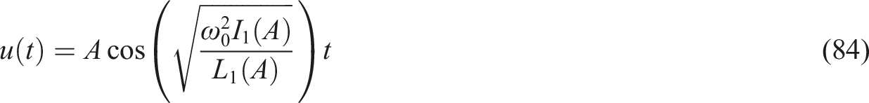
where $I_0\left(A\right)$ , $I_1\left(A\right)$ and $L_1\left(A\right)$ are the modified Bessel functions of zero-order, first-order and Struve function of the first-order, respectively. It is noted that the solution (81) is convergent for small A, while the solution (84) is convergent for large amplitude $A$ as seen from Figures 6 and 7. To perform the best solution, that is converged to the numerical solution for all amplitude $A$ (small or large), the frequency of equation (77) can be written as sought in (76) in the configuration

$${\omega }^2\left(A\right)=\underset{u\to \frac{1}{2}A}{\lim }\left(\frac{\tanh u}{u}\right)=\underset{u\to \frac{1}{2}A}{\lim }\left(\frac{\sinh u}{u\hspace{0.17em}\cosh u}\right)$$

(85)

Figure 6.

Contrasting the numerical solution of equation (77) (red-dash curve), the analytical solution (81) (blue-dot curve), and the analytical solution (83) (green-dot curve) for a system having the coefficients ${\omega }_0=1,\hspace{0.17em}A=.3$

Figure 7.

Contrasting the numerical solution of equation (76) (red-dash curve), the analytical solution (81) (blue-dot curve), and the analytical solution (83) (green-dot curve) for a system having the coefficients. ${\omega }_0=1,\hspace{0.17em}A=\mathrm{1.22.}$

Regarding this formula, the right-hand side is composed of an odd function in the numerator and an odd function in the dominator of (85); therefore, the integrative formula for the frequency $\omega$ can be sought as

$${\omega }^2\left(A\right)={\omega }_0^2\left(\frac{\frac{2}{T}{\displaystyle {\int }_0^T\left(\sinh \widehat{u}\right)\cos \hspace{0.17em}\omega tdt}}{\frac{2}{T}{\displaystyle {\int }_0^T\left(\widehat{u}\cosh \widehat{u}\right)\cos \hspace{0.17em}\omega tdt}}\right)=\frac{{\omega }_0^2{I}_1\left(A\right)}{I_1\left(A\right)+A{I}_2\left(A\right)}$$

(86)

This result is equivalent to those obtained by Galerkin’s formula to estimate the frequency. Applying the trial solution used above, then Galerkin’s approach leads to

$$\frac{1}{T}{\displaystyle {\int }_0^T\left(\widehat{\ddot{u}}\cosh \widehat{u}+{\omega }_0^2\sinh \widehat{u}\right)\cos \omega t}={\omega }_0^2{I}_1\left(A\right)-{\omega }^2\left(I_1\left(A\right)+A{I}_2\left(A\right)\right)=0$$

(87)

Thus, the frequency ${\omega }^2\left(A\right)$ is given as in (86). Consequently, the solution of equation (77) can be sought in the form

$$u\left(t\right)=A\hspace{0.17em}\cos \sqrt{\frac{{\omega }_0^2{I}_1\left(A\right)}{I_1\left(A\right)+A{I}_2\left(A\right)}}t$$

(88)

If the function $\tanh u$ has been replaced by $\tan u$ , then the effective solution, as mentioned above, has the following form

$$u\left(t\right)=A\hspace{0.17em}\cos \hspace{0.17em}\varpi t$$

(89)

where

$${\varpi }^2=\frac{{\omega }_0^2{J}_1\left(A\right)}{J_1\left(A\right)-A{J}_2\left(A\right)}$$

(90)

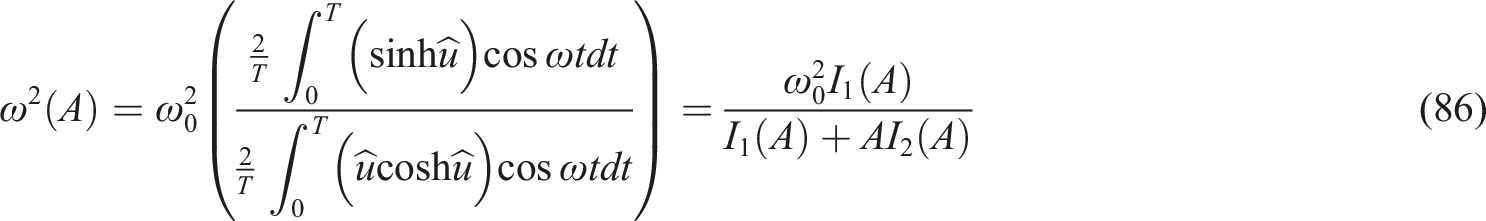
Comparison of the analytical solutions (83), (84), and (87) with the exact numerical solution for various cases are illustrated in Figures 6–8. The calculations of solutions (81) and (82) are collected together with the numerical solution in one graph. Figure 6 is plotted for small amplitude A $\left(A<<1\right)$ , while Figure 7 for $\left(A>1\right)$ . Figure 8 is assigned to the solution (73) for various amplitude values. It is observed that, in Figure 6, small values of the amplitude $A$ ( $A=0.3$ ) make the curve of the solution (81) in agreement with the numerical solution. The error will slowly increase as the amplitude $A$ increases. Much increase in the amplitude $A$ leads to an increase in the error. It is shown from Figure 7 that in the case of larger values of the amplitude $A>1$ , the solution (83) has much agreement with the numerical solution. The best solution (88) is displayed in Figure 8. This graph is plotted for various values of the amplitude $A$ for the sake of comparison. It is observed that the solution (88) has an excellent agreement with the numerical solution for all values of the amplitude $A$ .

Figure 8.

Comparison the solution (88) (blue-dot curve) with the numerical solution of equation (77) (red-dash curve), for ${\omega }_0=1,\hspace{0.17em}A=0.1,\hspace{0.17em}0.4,\hspace{0.17em}0.7,\hspace{0.17em}1,\hspace{0.17em}1.5$

The simplest approach for the frequency of nonlinear singular oscillators

The current section deals with estimating the frequency of a nonlinear singular oscillator. The frequency–amplitude relationship of singular oscillators, will be performed. The obtained results are compared with those obtained by Galerkin’s method to show the effectiveness of the proposed technique for solving the singular problem.

For the specially interested oscillator

$$\ddot{u}+\frac{1}{u}=0;\hspace{1em}u\left(0\right)=A,\hspace{1em}\dot{u}\left(0\right)=0$$

(91)

Estimating the frequency ${\omega }^2$ by direct application of He’s frequency formula yields

$${\omega }^2={f^{\prime }|}_{u=\frac{1}{2}A}=-{\frac{1}{u^2}|}_{u=\frac{1}{2}A}=-\frac{4}{A^2}$$

(92)

This result makes $\omega$ to be imaginary and so there is no oscillation. Instead of the direct application, the singular expansion of the restoring force $f\left(u\right)=1/u$ may be rewritten as

$$f\left(u\right)=\frac{u}{u^2}$$

(93)

It is noted that the restoring force is given in (93) is called the enhanced restoring force. The enhanced technique is used only to make an odd numerator and an even dominator; the original potential function is used to estimate the frequency directly. According to (93), the frequency $\omega$ is estimated as

$${\omega }^2={\frac{f\left(u\right)}{u}|}_{u=\frac{1}{2}A}$$

(94)

Employing (93) into (94) yields a rational expression with two odd polynomials into the numerator and the denominator. Consequently, the He’s differentiative approach will be applied to both the numerator and the denominator individually. Accordingly, the frequency is found to be

$${\omega }^2={\frac{D_{u}u}{D_u{u}^3}|}_{u=\frac{1}{2}A}=\frac{4}{3A^2}$$

(95)

In the other words, the frequency in the integrative form is given by

$${\omega }^2=\frac{{\displaystyle {\int }_0^{T}u\hspace{0.17em}\cos \hspace{0.17em}\omega tdt}}{{\displaystyle {\int }_0^T{u}^3\cos \hspace{0.17em}\omega tdt}}=\frac{1}{\frac{3}{4}{A}^2}$$

(96)

This is only a qualified frequency of the singular oscillator (91).

The verified by Galerkin’s formula

In this case, the Galerkin technology ⁵⁰ is more suitable to estimate the frequency. The Galerkin technology is seeking the frequency via the vanishing of the weight residual integral. Consider that the trial solution has the form

$$u\left(t\right)=A\hspace{0.17em}\cos \hspace{0.17em}\omega t$$

(97)

where $\omega$ is the oscillator frequency to be determined. It is convenient to write equation (91) in the non-singular form by multiplying both sides by $u^2$ . By introducing the weight function in the form $\cos \omega t$ , the frequency comes through the following condition

$$\frac{2}{AT}{\displaystyle {\int }_0^T\left(\ddot{u}{u}^2+u\right)\cos \hspace{0.17em}\omega tdt}=0$$

(98)

Inserting (96) into (97) yields

$$\frac{2}{AT}{\displaystyle {\int }_0^T\left(-{\omega }^2{A}^3{\cos }^3\omega t+A\hspace{0.17em}\cos \hspace{0.17em}\omega t\right)\cos \hspace{0.17em}\omega tdt=-1+\frac{3}{4}{A}^2{\omega }^2=0}$$

(99)

This is the same as that obtained in (95) and (96). At this end, the approximate solution has the form

$$y\left(t\right)=A\hspace{0.17em}\cos \left(\frac{\sqrt{3}}{2A}\right)t$$

(100)

The comparison between the frequency obtained in (95) and that obtained by Galerkin’s method indicated that the simplest differential form performed by He ⁵¹ cannot be applied directly to rational potential functions.

Remark

For the anti-cubic nonlinearity

$$\ddot{u}+\frac{1}{u^3}=0;\hspace{0.17em}\hspace{0.17em}u\left(0\right)=A,\hspace{0.17em}\dot{u}\left(0\right)=0.$$

(101)

By enhancing the restoring force $f\left(u\right)=u/u^4$ , the frequency is sought to be

$${\omega }^2={\frac{f\left(u\right)}{u}|}_{u=\frac{1}{2}A}=\underset{u\to \frac{1}{2}A}{\lim }\left(\frac{D_{u}u}{1/2!u{D}_u^2{u}^5}\right)=\frac{8}{5A^4}$$

(102)

To the general singular case

$$\ddot{u}+\frac{1}{u^{2n+1}}=0;\hspace{1em}u\left(0\right)=A,\hspace{1em}\dot{u}\left(0\right)=0$$

(103)

The enhanced restoring force is $f\left(u\right)=u/u^{2n+2}$ ; therefore, the frequency can be estimated as

$${\omega }^2={\frac{f\left(u\right)}{u}|}_{u=\frac{1}{2}A}=\underset{u\to \frac{1}{2}A}{\lim }\frac{D_{u}u}{\frac{1}{\left(n+1\right)!}{u}^n{D}_u^{n+1}{u}^{2n+3}}$$

(104)

Consider the following singular with anti-cubic and anti quintic oscillator

$$\ddot{u}+\frac{1}{u}+\frac{1}{u^3}+\frac{1}{u^5}=0;\hspace{1em}u\left(0\right)=A,\hspace{1em}\dot{u}\left(0\right)=0$$

(105)

It is seen that the enhanced restoring force can be sought in the form

$$f\left(u\right)=\frac{u+u^3+u^5}{u^6}$$

(106)

Consequently, the frequency is performed as

$${\omega }^2={\frac{f\left(u\right)}{u}|}_{u=\frac{1}{2}A}=\underset{u\to \frac{1}{2}A}{\lim }\left(\frac{\frac{d}{du}\left(u+u^3\right)+1/2!u\frac{d^2}{d{u}^2}{u}^5}{1/3!u^2\frac{d^3}{d{u}^3}{u}^7}\right)=\frac{1+\frac{3}{4}{A}^2+\frac{5}{8}{A}^4}{\frac{35}{64}{A}^6}$$

(107)

The same results can be obtained using the Galerkin method to estimate the frequency

$$\frac{2}{A\hspace{0.17em}T}{\displaystyle {\int }_0^T\left(\ddot{u}{u}^6+u^5+u^3+u\right)\cos \hspace{0.17em}\omega tdt}=\left(\frac{5}{8}{A}^4+\frac{3}{4}{A}^2+1\right)-\frac{35}{64}{A}^6{\omega }^2=0$$

(108)

Accordingly, the approximate solution has the form

$$u\left(t\right)=A\hspace{0.17em}\cos \sqrt{\frac{64+48A^2+40A^4}{35A^6}}t$$

(109)

Remark:

If the anti-odd powers in equation (105) have been extended to the general case, the infinite summation leads to

$$\ddot{u}+\frac{u}{u^2-1}=0$$

(110)

Hence, its frequency is

$${\omega }^2={\frac{f\left(u\right)}{u}|}_{u=\frac{1}{2}A}=\underset{u\to \frac{1}{2}A}{\lim }\left(\frac{D_{u}u}{D_u\left(u^3-u\right)}\right)=\frac{1}{\frac{3}{4}{A}^2-1}$$

(111)

It is worthwhile to an observer that the result can be obtained by Galerkin’s method.

Consider the following Duffing with an anti-cubic oscillator

$$\ddot{u}+u+u^3+\frac{1}{u^3}=0;\hspace{1em}u\left(0\right)=A,\hspace{1em}\dot{u}\left(0\right)=0$$

(112)

One can say that the restoring force is composed of two parts

$$f\left(u\right)=f_1\left(u\right)+f{}_2\left(u\right)$$

(113)

where $f_1\left(u\right)$ is selected to be the original Duffing’s potential and $f{}_2\left(u\right)$ is the anti-cubic function. So the frequency can be estimated as

$${\omega }^2=\underset{u\to \frac{1}{2}A}{\lim }\left(D_u{f}_1\left(u\right)+\frac{f_2\left(u\right)}{u}\right)=\underset{u\to \frac{1}{2}A}{\lim }\left(D_u\left(u+u^3\right)+\frac{D_{u}u}{1/2!u{D}_u^2{u}^5}\right)=1+\frac{3}{4}{A}^2+\frac{8}{5A^4}$$

(114)

But this result is not equivalent to the frequency obtained by Galerkin’s method. The accurate approach selects the enhanced general restoring force $f\left(u\right)$ as

$$f\left(u\right)=\frac{u+u^5+u^7}{u^4}$$

(115)

Consequently, the frequency formula is given by

$${\omega }^2=\underset{u\to \frac{1}{2}A}{\lim }\frac{f\left(u\right)}{u}=\underset{u\to \frac{1}{2}A}{\lim }\frac{D_{u}u+1/2!u{D}_u^2{u}^5+1/3!u^2{D}_u^3{u}^7}{1/2!u{D}_u^2{u}^5}=\frac{1+\frac{5}{8}{A}^4+\frac{35}{64}{A}^6}{\frac{5}{8}{A}^4}$$

(116)

This is identical to those performed by Galerkin’s method. The solution is found to have the form

$$u=A\hspace{0.17em}\cos \left(\sqrt{\frac{8}{5}{A}^{-4}+1+\frac{7}{8}{A}^2}t\right)$$

(117)

Conclusion

The present procedures are efficient for constructing periodic solutions to the generalized Helmholtz–Duffing oscillator and its family. The nonlinear terms of the oscillator have been split into odd and even sections which are converted to a non-homogenous linear harmonic equation. The oscillator frequency has been derived using the secular function (odd function), and the non-secular function (even function) is used to derive the inhomogeneity of the harmonic oscillator. Three styles of nonlinear frequency and the inhomogeneity part are derived in this approach. The frequency in the differentiative structure is organized in the generalization form of He’s formula. In addition, the frequency in the format of power series is derived. Further, the frequency in the integrative configuration is also derived. The approach is exercised to the Toda and the Z-S oscillators. The oscillators with the relative structure of the restoring force such as the Tangent oscillator are discussed with two additional examples. The proposal has been extended to cover the singular oscillator. The current paper extends the guide to the applicability of the frequency formulas for all nonlinear oscillators involving quadratic or even functions or singularity that are established in engineering and physics applications. It is worthwhile to indicate that the integrative formula for the frequency (34) is the simplest formularization of the frequency–amplitude relationship. As was said, “The simpler the calculation is the best for the nonlinear vibration theory.” This paper proposes possibly the simplest method for quickly testing the frequency property of a nonlinear oscillator; the one‐step solution produces a highly accurate result, which is quite agreeable.