Successive approximate solutions for nonlinear oscillation and improvement of the solution accuracy with efficient non-perturbative technique

Abstract

In the present study, several successive approximate solutions of the nonlinear oscillator are derived by using the efficient frequency formula. A systematical analysis of the formulation of the nonlinear frequency helps to establish a general periodic solution. Each approximation represents, individually, the solution of the nonlinear oscillator. For the optimal design and accurate prediction of structural behavior, a new optimizer is demonstrated for efficient solutions. The classical Duffing frequency formula has been modified. The numerical calculations show high agreement with the exact frequency. The justifiability of the obtained solutions is confirmed by comparison with the numerical solution. It is shown that the enhanced solution is accurate for large amplitudes and is not restricted to oscillations that have small amplitudes. The new approach can provide a perfect approximation for the nonlinear oscillation.

Introduction

A general simple form of the nonlinear oscillator can be described as

$\ddot{u}+F\left(u\right)=0;\hspace{0.17em}u\left(0\right)=A\&\dot{u}\left(0\right)=0,$

(1)

where the over dot denotes the derivative concerning time t, and $F\left(u\right)$ is an odd nonlinear term. It can be verified that equation (1) can be rewritten in the following configuration

$\ddot{u}+\left(\frac{F\left(u\right)}{u}\right)u=0,$

(2)

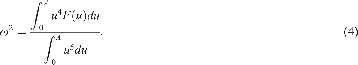
where the ratio $\frac{F\left(u\right)}{u}$ represents the stiffness due to the odd nonlinearity. In the simplest representation, He ¹ rewrote equation (2) in the form of

$\ddot{u}+{\omega }^2\left(A\right)u=0,$

(3)

where $A$ and $\omega$ are the amplitude and the frequency of the nonlinear oscillation, respectively. The application of Galerkin’s method and the least square technique ² has successfully evaluated the frequency ${\omega }^2\left(A\right)$ . There are many analytical available methods in the literature^3–8 to estimate the frequency. Following the classical procedure of He’s formula, ¹ Younesiana et al. ⁹ have considered the generalized Duffing equation having $F\left(u\right)={\displaystyle \sum }_{n=0}^N{a}_{2n+1}{u}^{2n+1}$ . Based on the weighted residuals, the frequency was performed. Based on the energy balance method, the same authors ⁹ obtained an alternative frequency formula. Utilizing the basic idea of the Energy Balance Method, Mahmoud Bayat et al. ¹⁰ established another form of frequency formula. The same procedure of Ref. 9 has been used by Molla and Alam ¹¹ to determine the frequency-amplitude relationship, and they suggested a procedure that depends on the energy balance method to obtain a higher-order approximate solution. Their procedure led to complicated coupled nonlinear algebraic equations. Following these authors, He et al. ¹² used the Hamiltonian-based formulation to determine the frequency property of the nonlinear oscillator for the cubic Duffing equation. Following Younesiana et al. ⁹ and He et al. ¹² and Mahmoud Bayat et al., ¹⁰ Hongjin Ma ¹³ derived two formulations for the frequency-amplitude formulation. A modified frequency formulation for nonlinear oscillators has been suggested by He and Liu for a fractal vibration in a porous medium ¹⁴

${\omega }^2=\frac{\underset{0}{\overset{A}{{\displaystyle \int }}}{u}^{4}F\left(u\right)du}{\underset{0}{\overset{A}{{\displaystyle \int }}}{u}^{5}du}.$

(4)

He^15–17 has proposed a simple formalism to derive the frequency from the nonlinear stiffens $F\left(u\right)/u$

${\omega }^2\left(A\right)={\frac{dF\left(u\right)}{du}|}_{u=\overline{u}}.$

(5)

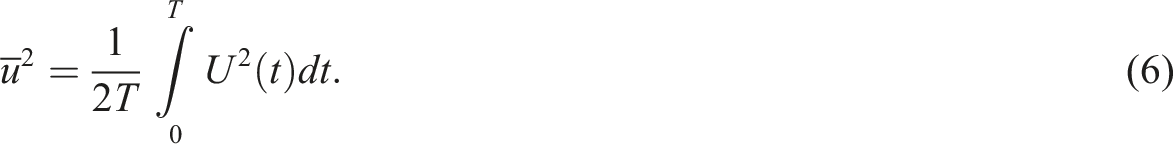
It is worthwhile to note that the located point $\overline{u}$ is estimated depending on the suggestion of a trial solution $U\left(t\right)$ that satisfies the given initial conditions. It is noted that the least mean square criterion of the displacement is defined as

${\overline{u}}^2=\frac{1}{2T}\underset{0}{\overset{T}{{\displaystyle \int }}}{U}^2\left(t\right)dt.$

(6)

Usually, the trial solution that corresponds to the initial conditions given by equation (1) is assumed to be

$U\left(t\right)=A\cos \omega t.$

(7)

This trial solution contains one unknown which is the frequency $\omega$ to be determined. Employing (7) into (6) yields

${\overline{u}}^2=\frac{1}{4}{A}^2.$

(8)

Inserting equation (8) into equation (5), the frequency will be determined as proposed by He.^15–17 This frequency formula has been modified by El-Dib ¹⁸ to become more accurate for strong nonlinear oscillators.

In a more general case, for non-conservative oscillators, El-Dib^19–21 follows formula (5) to establish the total frequency that covers the linear natural frequency, the nonlinear natural frequency, and the damped frequency. The frequency-amplitude relationship is derived by using He’s formula and was established in terms of the Bessel function for Gaylord’s oscillator. ²² He’s frequency formulation has been modified to cover the fractional nonlinear oscillator as given in Ref. 23. Also, this approach was applied to the parametric Gaylord’s oscillator with a discussion of the resonance response with the non-perturbative approach. ²⁴ Recently, a new perspective on He’s formula has discussed a delayed dynamical system by El-Dib et al. ²⁵ Further, application to He’s frequency formula for a class of fractal vibration systems has been proposed by Tian ²⁶ and El-Dib et al.^27,28 The fractal Toda oscillator has been established by the non-perturbative method and He’s frequency formula has been applied to determine the approximate analytical solution.^8,18

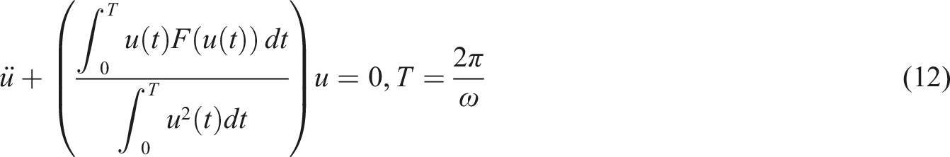
Recently, El-Dib ¹⁸ has established an extended frequency-amplitude in the differentiative form to cover the family of the Duffing oscillator with nonlinearity having the higher powers

${\omega }^2\left(A\right)=\underset{u\to \overline{u}}{\lim }{\displaystyle \sum }_{n=0}^{\infty }\frac{1}{n!}{a}_{2n+1}{u}^{n-1}{D}_u^n{u}^{2n+1},$

(9)

where $D_u^n$ refers to the $n^{th}$ order derivative concerning the variable $u$ . The first and the second terms in this formula give the simplest He’s frequency formula for the cubic Duffing equation.^15,16 Based on formula (9), the author of Ref. 18 established an equivalent formula in the power series form that is given by

${\omega }^2={\displaystyle \sum }_{n=0}^{\infty }{a}_{2n+1}\frac{\left(2n+1\right)\hspace{0.17em}!}{n!\times \left(n+1\right)\hspace{0.17em}!}{\overline{u}}^{2n},$

(10)

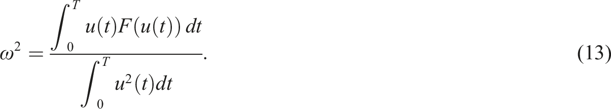
where $\overline{u}$ is the least mean square criterion of the displacement. ¹⁸ Returning to the nonlinear equation (2), it is rewritten in a new version as

$\ddot{u}+\left(\frac{uF\left(u\right)}{u^2}\right)u=0.$

(11)

Then, integrating the numerator and the denominator of the stiffens term concerning the variable $t$ , individually, from zero to $T$ , equation (11) becomes

$\ddot{u}+\left(\frac{\underset{0}{\overset{T}{{\displaystyle \int }}}u\left(t\right)F\left(u\left(t\right)\right)\hspace{0.17em}dt}{\underset{0}{\overset{T}{{\displaystyle \int }}}{u}^2\left(t\right)dt}\right)u=0,T=\frac{2\pi }{\omega }$

(12)

The comparison with equation (3) shows that the frequency ${\omega }^2$ arises in the form

${\omega }^2=\frac{\underset{0}{\overset{T}{{\displaystyle \int }}}u\left(t\right)F\left(u\left(t\right)\right)\hspace{0.17em}dt}{\underset{0}{\overset{T}{{\displaystyle \int }}}{u}^2\left(t\right)dt}.$

(13)

With a suitable chosen trial solution, doing the above integrals give the corresponding frequency. This formula was previously published by El-Dib ¹⁸ which is the best and most efficient formula and can be used for obtaining successive approximate solutions for the nonlinear oscillation (1). Formula (13) has a wide range of application in nonlinear oscillators. El-Dib ²⁹ used formula (13) to derive the frequency of the complex Helmholtz–Duffing oscillator.

It is worthwhile to observe that all the abovementioned frequency formulas cannot formulate the frequency corresponding to a successive process, except the frequency formula (13). Because the derivation of the equivalent frequency (13) depends on the trial solution, then for each trial solution, there is a corresponding frequency formula. If the frequency is determined, the successive approximate solution will be found to simulate the assumption of the trial solution. The process can be well-advanced with the appropriate trial solutions fulfilling essential initial conditions, making the computing procedure more efficient for accelerated convergence and beneficiating accuracy.^30,31

In the current paper, an analytical approximation that has been mentioned above will be presented to obtain several successive approximate periodic solutions depending on introducing several trial solutions; and by using the integrative expression (13), the frequency formula will be obtained.

Basic ideas of the successive approximate solutions

The derivation of the approximate solution of equation (1) with the efficient frequency approach depends on the suggestion of a trial solution that contains the unknown frequency $\omega$ , where the target is to determine this unknown. To illustrate the main target, the following cubic Duffing oscillator can be considered

$\ddot{u}+\alpha u+Q{u}^3=0;\hspace{0.17em}u\left(0\right)=A\&\dot{u}\left(0\right)=0,$

(14)

where $\alpha ,Q$ and $A$ are dimensionless physical quantities having numerical values.

A simple suitable trial solution (6) together with employing $F\left(u\right)=\alpha u+Q{u}^3$ , formula (13) yields the corresponding frequency. Let the obtained frequency be ${\omega }_0$

${\omega }_0=\sqrt{\alpha +\frac{3}{4}{A}^{2}Q}.$

(15)

Accordingly, the approximate solution is presented in the form

$u_0\left(t\right)=A\cos \left(\sqrt{\alpha +\frac{3}{4}{A}^{2}Q}\right)t=A\cos \left(\sqrt{\alpha +0.75A^{2}Q}\right)t.$

(16)

The accuracy of the present method can be seen by comparing it with the exact frequency^10,30

${\omega }_{ex}=\frac{\pi /2}{\underset{0}{\overset{\pi /2}{{\displaystyle \int }}}\frac{d\theta }{\sqrt{\alpha +\frac{1}{2}Q{A}^2\left({\mathit{cos}}^2\theta +1\right)}}}.$

(17)

The first extended of the suitable trial solution

The main question now is what the approximate solution of equation (1) is if the trial solution has been selected in another suitable form instead of (6).

Consider the trial solution that satisfies the initial conditions in the form

$U_1\left(t\right)=A\left[\cos {\omega }_{1}t+{\lambda }_0\left(\cos 3{\omega }_{1}t-\cos {\omega }_{1}t\right)\right],$

(18)

where ${\lambda }_0$ is an unknown constant. This form is selected to emulate the first-order solution obtained by the perturbation method. This suggestion contains two unknowns ${\omega }_1$ and ${\lambda }_0$ .

The trial solution (18) can be expected as

$U_1\left(t\right)=U_a\left(t\right)+U_b\left(t\right),$

(19)

where

$U_a\left(t\right)=A\left(1-{\lambda }_0\right)\cos {\omega }_{1}t\hspace{0.17em}\mathrm{a}\mathrm{n}\mathrm{d}\hspace{0.17em}{U}_b\left(t\right)=A{\lambda }_0\cos 3{\omega }_{1}t.$

(20)

The least square of the displacement is estimated for both functions $U_a\left(t\right)$ and $U_b\left(t\right)$ as follows:

${\overline{u}}_1^2=\frac{1}{2T}\underset{0}{\overset{T}{{\displaystyle \int }}}{U}_a^2\left(t\right)dt=\frac{1}{2T}\underset{0}{\overset{T}{{\displaystyle \int }}}{U}_b^2\left(t\right)dt.$

(21)

Employing (20) into (21), the integral corresponding $\cos {\omega }_{1}t$ gives

${\overline{u}}_1^2=\frac{1}{4}{A}^2{\left(1-{\lambda }_0\right)}^2.$

(22)

The integral corresponding $\cos 3{\omega }_{1}t$ leads to

${\overline{u}}_1^2=\frac{1}{4}{A}^2{\lambda }_0^2.$

(23)

Solving (22) with (23) yields

${\lambda }_0=\frac{1}{2}.$

(24)

Inserting equation (24) into equations (22) or (23), the least square of the displacement is found to be

${\overline{u}}_1^2=\frac{1}{4\times 2^2}{A}^2.$

(25)

Inserting equation (24) into equation (18) gives

$U_1\left(t\right)=\frac{1}{2}A\left(\cos {\omega }_{1}t+\cos 3{\omega }_{1}t\right).$

(26)

Employing equation (26) into the efficient frequency formula (13) to estimate ${\omega }_1$ yields

${\omega }_1^2=\frac{\underset{0}{\overset{T_1}{{\displaystyle \int }}}{U}_1\left(t\right)F\left(U_1\left(t\right)\right)\hspace{0.17em}dt}{\underset{0}{\overset{T_1}{{\displaystyle \int }}}{U}_1^2\left(t\right)dt};\hspace{0.17em}{T}_1=\frac{2\pi }{{\omega }_1}.$

(27)

Running the integrations in equation (27) gives

${\omega }_1^2=\alpha +\frac{11}{16}{A}^{2}Q=\alpha +0.6875A^{2}Q.$

(28)

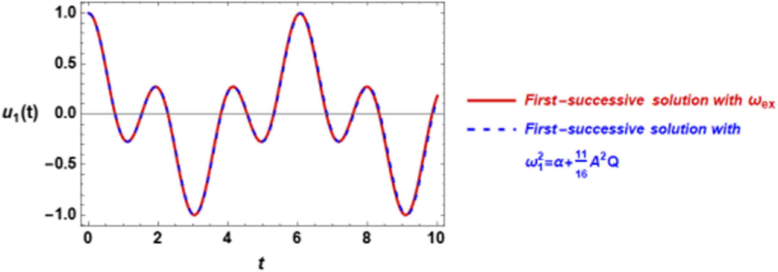
Accordingly, the successive approximate solution that simulates the trial solution (18) for the Duffing oscillator (14) gives

$u_1\left(t\right)=\frac{1}{2}A\left(\cos {\omega }_{1}t+\cos 3{\omega }_{1}t\right).$

(29)

The approximate solution due to the second extension of the suitable trial solution

In this section, the trial solution has been extended to become composed of $\cos \omega t,\cos 3\omega t$ and $\cos 5\omega t$ as described below.

Consider the trial solution in the form

$U_2\left(t\right)=A\left[\cos {\omega }_{2}t+{\lambda }_1\left(\cos 3{\omega }_{2}t-\cos {\omega }_{2}t\right)+{\lambda }_2\left(\cos 5{\omega }_{2}t-\cos {\omega }_{2}t\right)\right].$

(30)

This suggestion is with three unknowns ${\omega }_2,{\lambda }_1$ and ${\lambda }_2$ to be determined. If we proceed as mentioned in the above section, the following results will be obtained.

Both the unknowns ${\lambda }_1$ and ${\lambda }_2$ will be the same and have the value ${\lambda }_i=\frac{1}{3}$ , and the least square of the displacement is found to be

${\overline{u}}_2^2=\frac{1}{4}{A}^2{\lambda }_i^2=\frac{1}{4\times 3^2}{A}^2.$

(31)

Inserting ${\lambda }_i=\frac{1}{3}$ into equation (30), the trial solution becomes one unknown ${\omega }_2$

$U_2\left(t\right)=\frac{1}{3}A\left(\cos {\omega }_{2}t+\cos 3{\omega }_{2}t+\cos 5{\omega }_{2}t\right).$

(32)

The frequency ${\omega }_2$ is estimated by inserting equation (32) into formula (13) to yield

${\omega }_2^2=\alpha +\frac{73}{108}{A}^{2}Q=\alpha +0.675926A^{2}Q.$

(33)

Finally, the second successive approximate solution is

$u_2\left(t\right)=\frac{1}{3}A\left[\cos {\omega }_{2}t+\cos 3{\omega }_{2}t+\cos 5{\omega }_{2}t\right].$

(34)

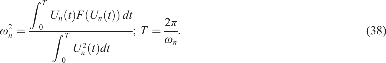
The solution for the sequential extension of the trial solution

To obtain the sequential extended approximate solution, one may assume that the serial trial solution has the form

$U_n\left(t\right)=A{\displaystyle \sum }_{r=0}^n{\lambda }_n\cos \left(2r+1\right){\omega }_{n}t,$

(35)

where ${\lambda }_n$ is called neutral weighting coefficients.

${\lambda }_n=\frac{2}{\left(n+1\right)AT}\underset{0}{\overset{T}{{\displaystyle \int }}}{U}_n\left(t\right)\cos \left(2r+1\right){\omega }_{n}tdt=\frac{1}{n+1}.$

(36)

Employing equation (36) into equation (35) reduced into one unknown as follows:

$U_n\left(t\right)=\frac{A}{n+1}{\displaystyle \sum }_{r=0}^n\cos \left(2r+1\right){\omega }_{n}t.$

(37)

Inserting (37) into formula (13) yields the frequency ${\omega }_n$ in the form

${\omega }_n^2=\frac{\underset{0}{\overset{T}{{\displaystyle \int }}}{U}_n\left(t\right)F\left(U_n\left(t\right)\right)\hspace{0.17em}dt}{\underset{0}{\overset{T}{{\displaystyle \int }}}{U}_n^2\left(t\right)dt};\hspace{0.17em}T=\frac{2\pi }{{\omega }_n}.$

(38)

The serial successive approximate solution is given by

$u_n\left(t\right)=\frac{A}{n+1}{\displaystyle \sum }_{r=0}^n\cos \left(2r+1\right){\omega }_{n}t.$

(39)

This formula gives the approximate solution to any serial required for the nonlinear function $\left(u\right)$ .

Applying the abovementioned information for $=3$ , the third successive approximation can be obtained in the form

$u_3\left(t\right)=\frac{1}{4}A\left[\cos {\omega }_{3}t+\cos 3{\omega }_{3}t+\cos 5{\omega }_{3}t+\cos 7{\omega }_{3}t\right],$

(40)

where

${\omega }_3^2=\alpha +\frac{43}{64}{A}^{2}Q=\alpha +0.671875A^{2}Q,$

(41)

and so on.

The Helmholtz–Duffing oscillator

It is noted that the nonlinear function $F\left(u\right)$ is assumed to be only composed of all the secular terms. If the nonlinear oscillator is constructed of non-secular terms $g\left(u\right)$ besides the secular terms $F\left(u\right)$ as given below

$\ddot{u}+F\left(u\right)=g\left(u\right);\hspace{0.17em}u\left(0\right)=A\&\dot{u}\left(0\right)=0.$

(42)

This is the Helmholtz–Duffing oscillator. For example, consider the functions $F\left(u\right)$ and $g\left(u\right)$ having the following forms

$F\left(u\right)=\alpha u+Q{u}^3,g\left(u\right)=\beta u^2.$

(43)

where the constant $\beta$ is the coefficient of the non-secular term.

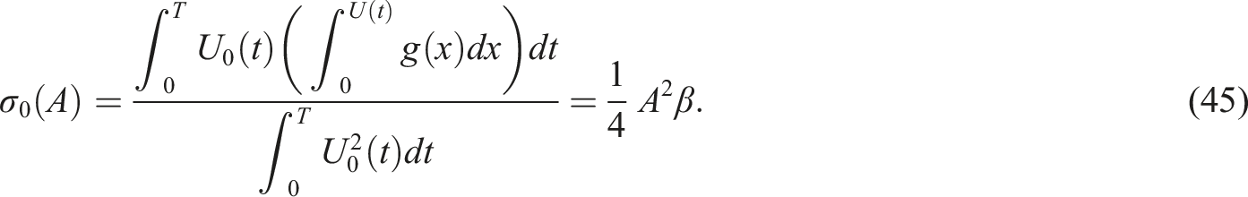
The zero-serial solution

The zero-serial solution of the Helmholtz–Duffing oscillator (42) utilizing the non-perturbative approach ¹⁸ is given by

$u_0\left(t\right)=\left(A-\frac{{\sigma }_0\left(A\right)}{{\omega }_0^2}\right)\cos {\omega }_{0}t+\frac{{\sigma }_0\left(A\right)}{{\omega }_0^2}.$

(44)

where ${\omega }_0$ is as given in equation (15), while ${\sigma }_0\left(A\right)$ is obtained in the form

${\sigma }_0\left(A\right)=\frac{\underset{0}{\overset{T}{{\displaystyle \int }}}{U}_0\left(t\right)\left(\underset{0}{\overset{U\left(t\right)}{{\displaystyle \int }}}g\left(x\right)dx\right)dt}{\underset{0}{\overset{T}{{\displaystyle \int }}}{U}_0^2\left(t\right)dt}=\frac{1}{4}{A}^2\beta .$

(45)

This solution is identical to those obtained in Ref. 18.

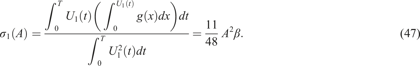
The first-serial successive solution

When $n=1$ is inserted into equations (35)–(42), the first-serial successive solution for the oscillator (42) has the form

$u_1\left(t\right)=\frac{1}{2}\left(A-\frac{{\sigma }_1\left(A\right)}{{\omega }_1^2}\right)\left(\cos {\omega }_{1}t+\cos 3{\omega }_{1}t\right)+\frac{{\sigma }_1\left(A\right)}{{\omega }_1^2},$

(46)

where ${\omega }_1$ is as given by equation (28), while ${\sigma }_1\left(A\right)$ is estimated to be

${\sigma }_1\left(A\right)=\frac{\underset{0}{\overset{T}{{\displaystyle \int }}}{U}_1\left(t\right)\left(\underset{0}{\overset{U_1\left(t\right)}{{\displaystyle \int }}}g\left(x\right)dx\right)dt}{\underset{0}{\overset{T}{{\displaystyle \int }}}{U}_1^2\left(t\right)dt}=\frac{11}{48}{A}^2\beta .$

(47)

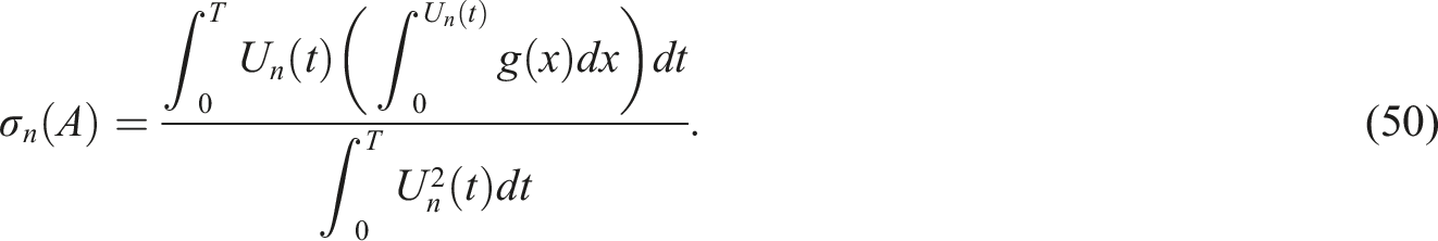
Similarly, the second-serial successive solution for the Helmholtz–Duffing oscillation (42) is

$u_2\left(t\right)=\frac{1}{3}\left(A-\frac{{\sigma }_2\left(A\right)}{{\omega }_2^2}\right)\left(\cos {\omega }_{2}t+\cos 3{\omega }_{2}t+\cos 5{\omega }_{2}t\right)+\frac{{\sigma }_2\left(A\right)}{{\omega }_2^2},$

(48)

where ${\sigma }_2\left(A\right)$ is estimated to be ${\sigma }_2\left(A\right)=\frac{73}{324}{A}^2\beta$ .

Accordingly, the general successive solution of (42) has the form

$u_n\left(t\right)=\frac{1}{n+1}\left(A-\frac{{\sigma }_n\left(A\right)}{{\omega }_n^2}\right){\displaystyle \sum }_{r=0}^n\cos \left(2r+1\right){\omega }_{n}t+\frac{{\sigma }_n\left(A\right)}{{\omega }_n^2},$

(49)

where ${\sigma }_n\left(A\right)$ is established using the non-secular function $g\left(u\right)$ which was estimated by El-Dib ¹⁶ to have the form

${\sigma }_n\left(A\right)=\frac{\underset{0}{\overset{T}{{\displaystyle \int }}}{U}_n\left(t\right)\left(\underset{0}{\overset{U_n\left(t\right)}{{\displaystyle \int }}}g\left(x\right)dx\right)dt}{\underset{0}{\overset{T}{{\displaystyle \int }}}{U}_n^2\left(t\right)dt}.$

(50)

Numerical illustrations and discussion

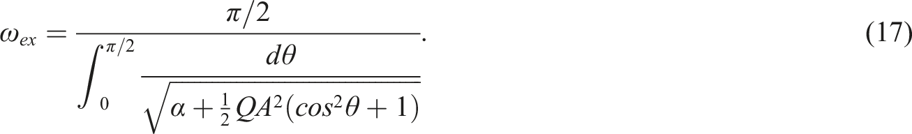
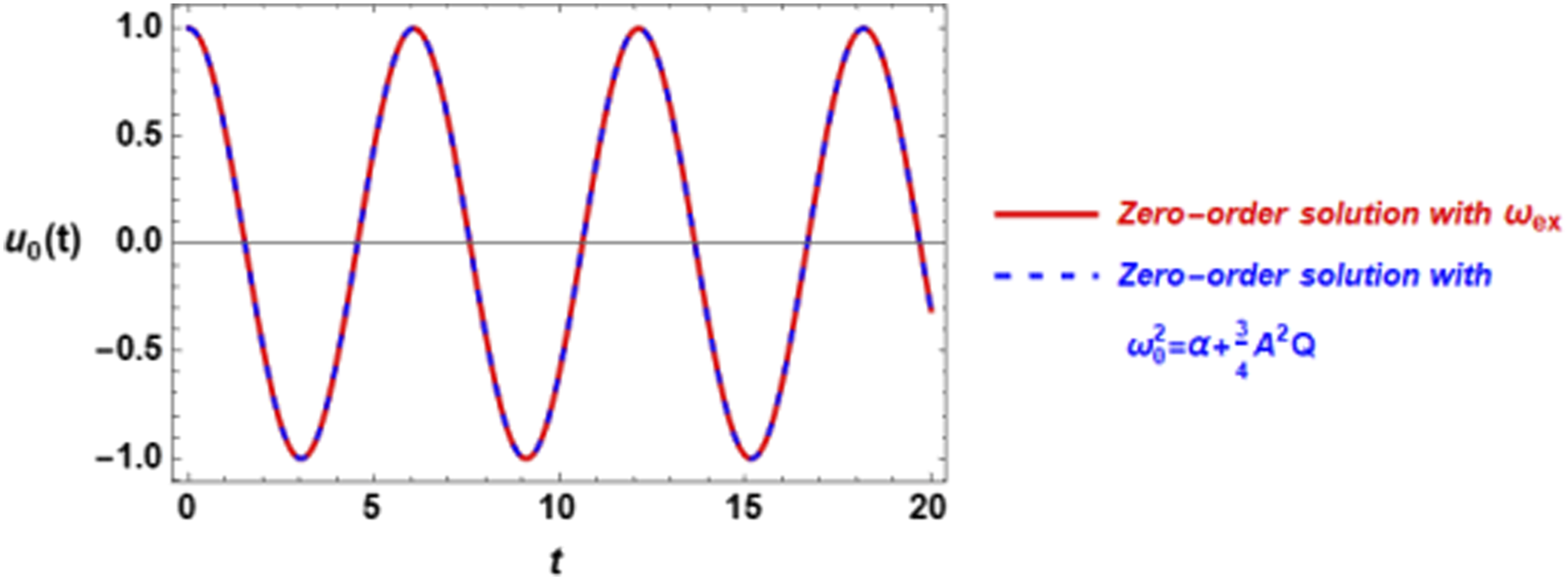
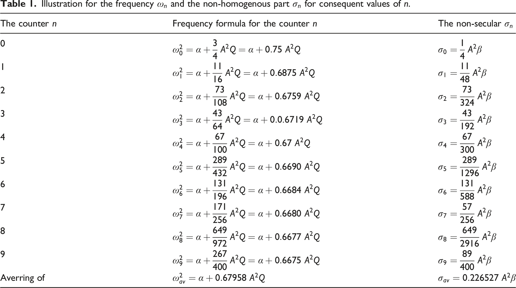
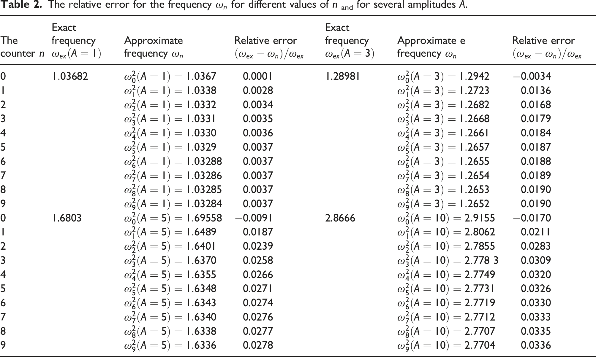
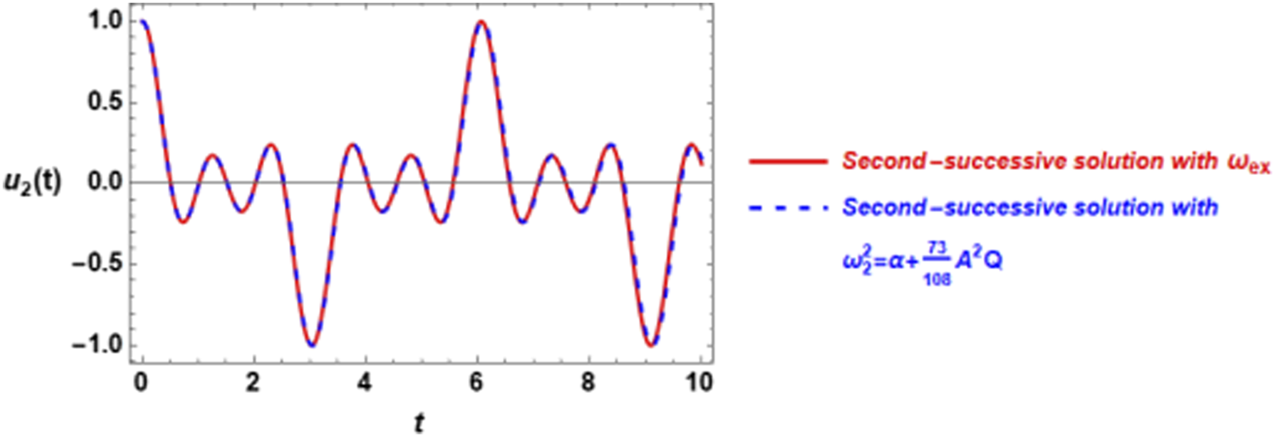
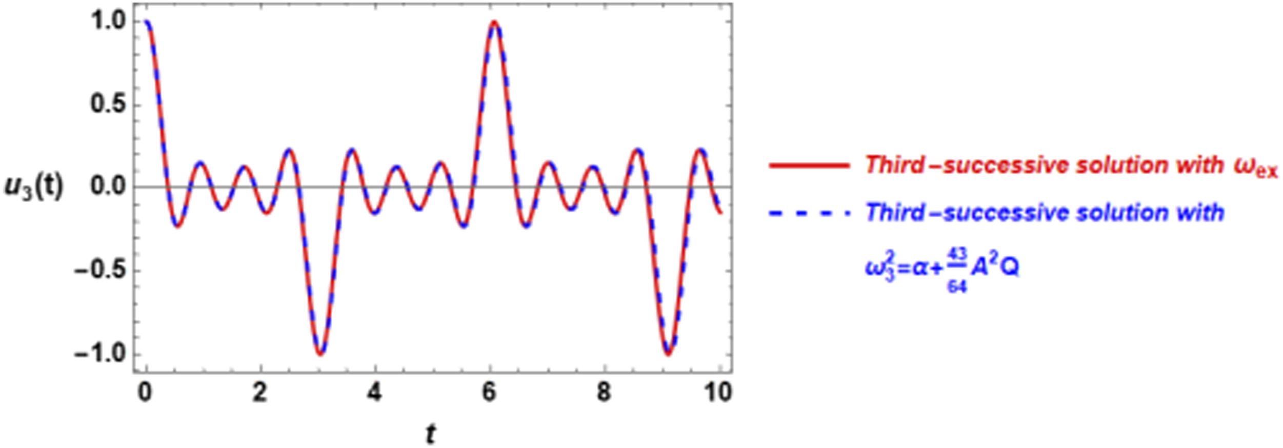
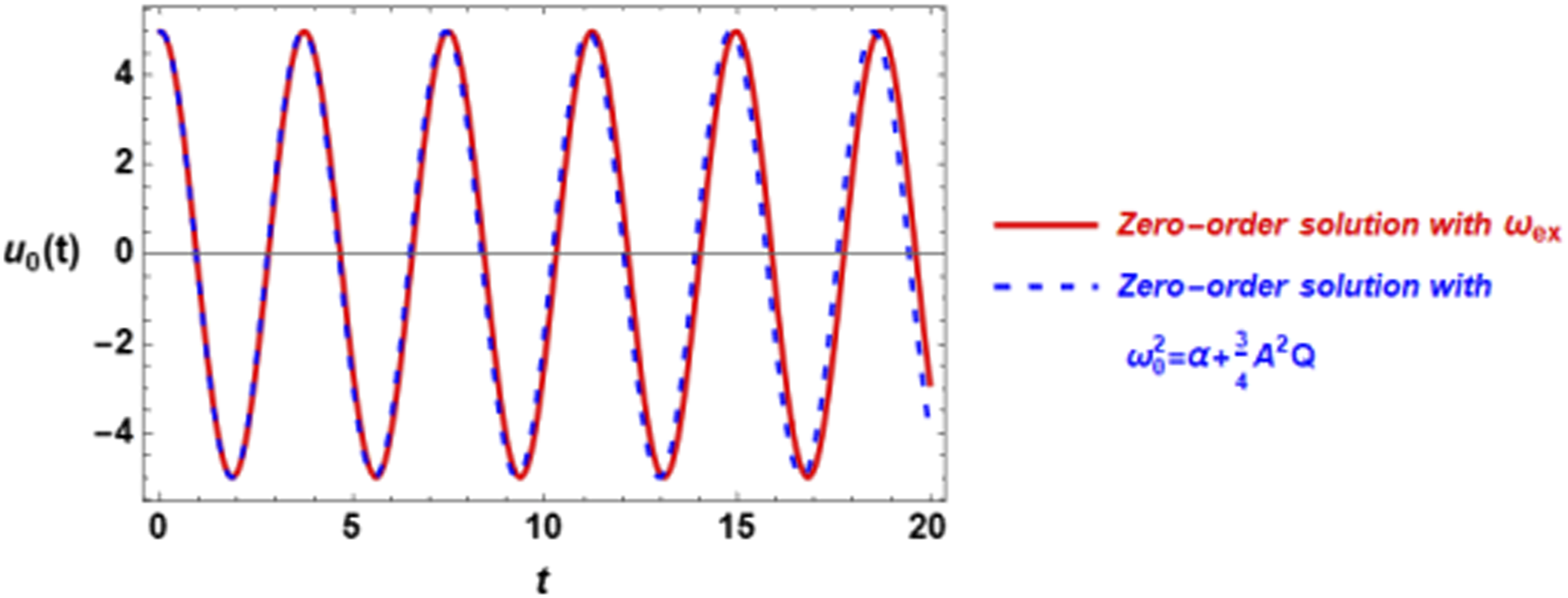
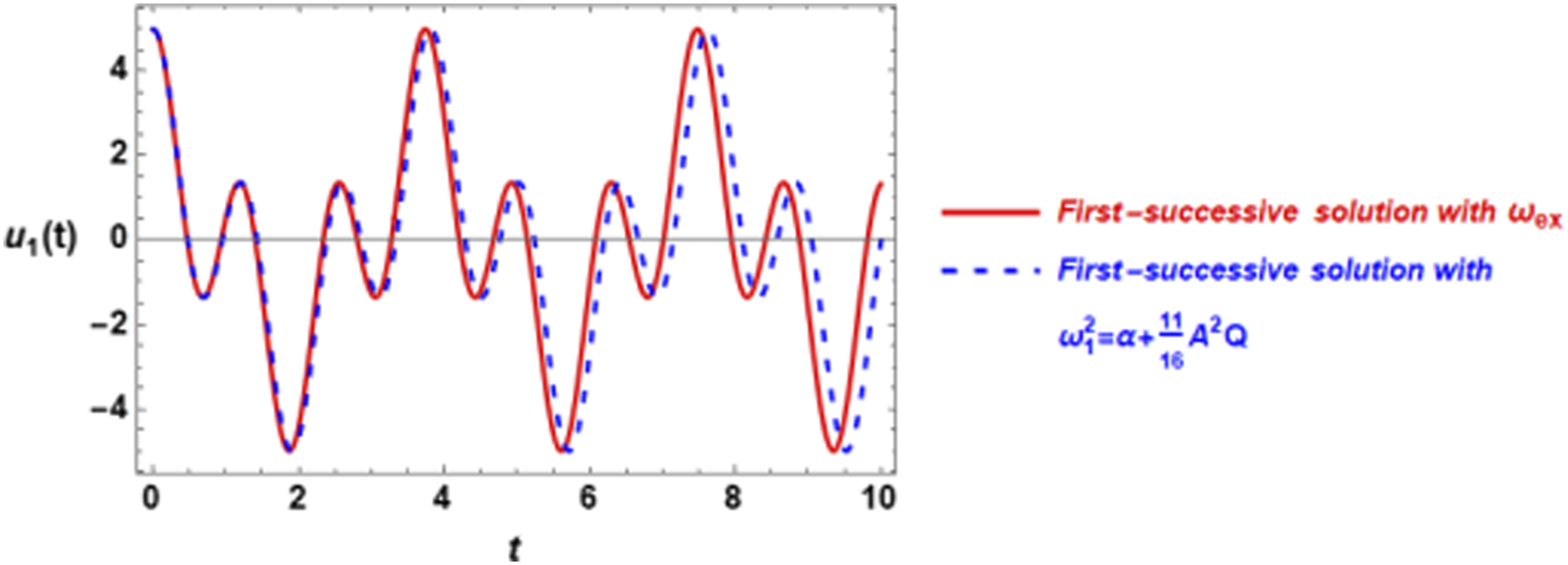
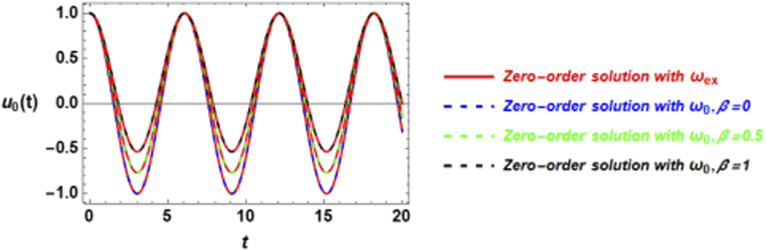
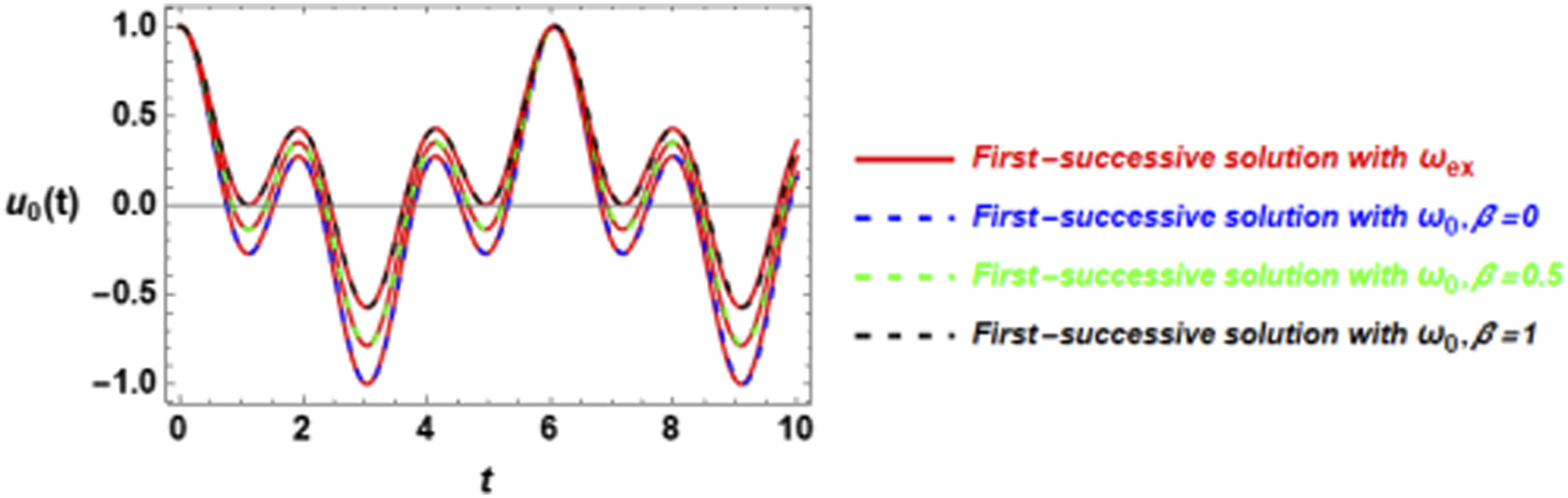
The zero-serial solution approximate solution (16) is plotted in Figure 1 to compare the solution with the exact frequency ${\omega }_{ex}$ of the solution, using the approximate frequency of the zero-serial approximation ${\omega }_0$ . Table 1 illustrates the frequency ${\omega }_n$ and ${\sigma }_n$ different values of $n$ . It is shown that as the serial number increases, the approximation accuracy of frequency deteriorates. Investigating the frequency obtained in Table 2 reveals the important point that ${\omega }_n^2$ seems to tend to a constant value as $n$ increases, especially for large $n$ . These values of the frequency are simulated as the exact value for small amplitude $A\left(A=1\right)$ . As the amplitude is increased, the relative error increases. This means that the present approach works well for $\le 1$ . The comparison of the exact frequency with the approximate frequency for the first, the second, and the third-serial successive solution is displayed in Figures 1–4, respectively. The calculations are made for the system given in Figure 1. Figures 5 and 6 are made for the system of Figure 1 except that the amplitude is chosen to be large as A $=5$ .

Figure 1.

Illustration of the approximate solution $u_0\left(t\right)$ to Duffing equation (14) for $\alpha =1,Q=0.1$ and $A=1$ . The relative error for the frequency ${\omega }_0$ is $0.0001$ .

Table 1.

Illustration for the frequency ${\omega }_n$ and the non-homogenous part ${\sigma }_n$ for consequent values of n.

The counter $n$	Frequency formula for the counter $n$	The non-secular ${\sigma }_n$
0	${\omega }_0^2=\alpha +\frac{3}{4} A^{2}Q=\alpha +0.75 A^{2}Q$	${\sigma }_0=\frac{1}{4} A^2\beta$
1	${\omega }_1^2=\alpha +\frac{11}{16} A^{2}Q=\alpha +0.6875 A^{2}Q$	${\sigma }_1=\frac{11}{48} A^2\beta$
2	${\omega }_2^2=\alpha +\frac{73}{108} A^{2}Q=\alpha +0.6759 A^{2}Q$	${\sigma }_2=\frac{73}{324} A^2\beta$
3	${\omega }_3^2=\alpha +\frac{43}{64} A^{2}Q=\alpha +\mathrm{0.0.6719} A^{2}Q$	${\sigma }_3=\frac{43}{192} A^2\beta$
4	${\omega }_4^2=\alpha +\frac{67}{100} A^{2}Q=\alpha +0.67 A^{2}Q$	${\sigma }_4=\frac{67}{300} A^2\beta$
5	${\omega }_5^2=\alpha +\frac{289}{432} A^{2}Q=\alpha +0.6690 A^{2}Q$	${\sigma }_5=\frac{289}{1296} A^2\beta$
6	${\omega }_6^2=\alpha +\frac{131}{196} A^{2}Q=\alpha +0.6684 A^{2}Q$	${\sigma }_6=\frac{131}{588} A^2\beta$
7	${\omega }_7^2=\alpha +\frac{171}{256} A^{2}Q=\alpha +0.6680 A^{2}Q$	${\sigma }_7=\frac{57}{256} A^2\beta$
8	${\omega }_8^2=\alpha +\frac{649}{972} A^{2}Q=\alpha +0.6677 A^{2}Q$	${\sigma }_8=\frac{649}{2916} A^2\beta$
9	${\omega }_9^2=\alpha +\frac{267}{400} A^{2}Q=\alpha +0.6675 A^{2}Q$	${\sigma }_9=\frac{89}{400} A^2\beta$
Averring of	${\omega }_{av}^2=\alpha +0.67958 A^{2}Q$	${\sigma }_{av}=0.226527 A^2\beta$

Table 2.

The relative error for the frequency ${\omega }_n$ for different values of $n$ _and for several amplitudes A.

The counter $n$	Exact frequency ${\omega }_{ex}\left(A=1\right)$	Approximate frequency ${\omega }_n$	Relative error $\left({\omega }_{ex}-{\omega }_n\right)/{\omega }_{ex}$	Exact frequency ${\omega }_{ex}\left(A=3\right)$	Approximate e frequency ${\omega }_n$	Relative error $\left({\omega }_{ex}-{\omega }_n\right)/{\omega }_{ex}$
0	$1.03682$	${\omega }_0^2\left(A=1\right)=1.0367$	0.0001	1.28981	${\omega }_0^2\left(A=3\right)=1.2942$	−0.0034
1		${\omega }_1^2\left(A=1\right)=1.0338$	0.0028		${\omega }_1^2\left(A=3\right)=1.2723$	0.0136
2		${\omega }_2^2\left(A=1\right)=1.0332$	0.0034		${\omega }_2^2\left(A=3\right)=1.2682$	0.0168
3		${\omega }_3^2\left(A=1\right)=1.0331$	0.0035		${\omega }_3^2\left(A=3\right)=1.2668$	0.0179
4		${\omega }_4^2\left(A=1\right)=1.0330$	0.0036		${\omega }_4^2\left(A=3\right)=1.2661$	0.0184
5		${\omega }_5^2\left(A=1\right)=1.0329$	0.0037		${\omega }_5^2\left(A=3\right)=1.2657$	0.0187
6		${\omega }_6^2\left(A=1\right)=1.03288$	0.0037		${\omega }_6^2\left(A=3\right)=1.2655$	0.0188
7		${\omega }_7^2\left(A=1\right)=1.03286$	0.0037		${\omega }_7^2\left(A=3\right)=1.2654$	0.0189
8		${\omega }_8^2\left(A=1\right)=1.03285$	0.0037		${\omega }_8^2\left(A=3\right)=1.2653$	0.0190
9		${\omega }_9^2\left(A=1\right)=1.03284$	0.0037		${\omega }_9^2\left(A=3\right)=1.2652$	0.0190
0	1.6803	${\omega }_0^2\left(A=5\right)=1.69558$	−0.0091	2.8666	${\omega }_0^2\left(A=10\right)=2.9155$	−0.0170
1		${\omega }_1^2\left(A=5\right)=1.6489$	0.0187		${\omega }_1^2\left(A=10\right)=2.8062$	0.0211
2		${\omega }_2^2\left(A=5\right)=1.6401$	0.0239		${\omega }_2^2\left(A=10\right)=2.7855$	0.0283
3		${\omega }_3^2\left(A=5\right)=1.6370$	0.0258		${\omega }_3^2\left(A=10\right)=2.778 3$	0.0309
4		${\omega }_4^2\left(A=5\right)=1.6355$	0.0266		${\omega }_4^2\left(A=10\right)=2.7749$	0.0320
5		${\omega }_5^2\left(A=5\right)=1.6348$	0.0271		${\omega }_5^2\left(A=10\right)=2.7731$	0.0326
6		${\omega }_6^2\left(A=5\right)=1.6343$	0.0274		${\omega }_6^2\left(A=10\right)=2.7719$	0.0330
7		${\omega }_7^2\left(A=5\right)=1.6340$	0.0276		${\omega }_7^2\left(A=10\right)=2.7712$	0.0333
8		${\omega }_8^2\left(A=5\right)=1.6338$	0.0277		${\omega }_8^2\left(A=10\right)=2.7707$	0.0335
9		${\omega }_9^2\left(A=5\right)=1.6336$	0.0278		${\omega }_9^2\left(A=10\right)=2.7704$	0.0336

Figure 2.

Graphical representation of the $u_1\left(t\right)$ given by (30) for the same system as given in Figure 1. The relative error for ${\omega }_1$ is $0.0028$ .

Figure 3.

Graphical representation of the $u_2\left(t\right)$ for the same system as given in Figure 1. The relative error between ${\omega }_2$ is $0.0034$ .

Figure 4.

Graphical representation of the $u_3\left(t\right)$ for the same system as given in Figure 1.

Figure 5.

Illustration of the approximate solution $u_0\left(t\right)$ to Duffing equation (14) for $\alpha =1,Q=0.1$ and $A=5$ . The relative error for the frequency ${\omega }_0$ is $-0.0091$ .

Figure 6.

Graphical representation of the $u_1\left(t\right)$ given by (30) for the same system as given in Figure 5. The relative error for ${\omega }_1$ is $0.01871.$

As shown, there is a high agreement ${\omega }_0,{\omega }_1,{\omega }_2,{\omega }_3$ with the exact frequency given by equation (29), especially for $A\le 1$ . It is observed that when the serial of the successive solution increases, the solution becomes high oscillation. Although there is excellent agreement with the exact frequency, the noteworthy feature is that as n increases, the shape of the solution is farther away from the numerical solution shape. This note can be observed through the comparison of Figures 2–4 with Figure 1.

The illustration for the zero-serial solution (44) for the Helmholtz–Duffing oscillator (42) has been plotted in Figure 7, while the first-serial successive solution (47) is plotted in Figure 8. The two graphs are made for three sequence values of the parameter $\beta$ . Inspection of these graphs shows that the increase in $\beta$ has no implication in the periodic solution, but leads to a contraction or an extension in the amplitude length according to $\beta$ having positive or negative values, respectively.

Figure 7.

Graphical representation of the $u_0\left(t\right)$ given by (44) to illustrate in $\beta$ for the same system as given in Figure 1.

Figure 8.

Graphical representation of the $u_1\left(t\right)$ given by (46) for the same system as given in Figure 1.

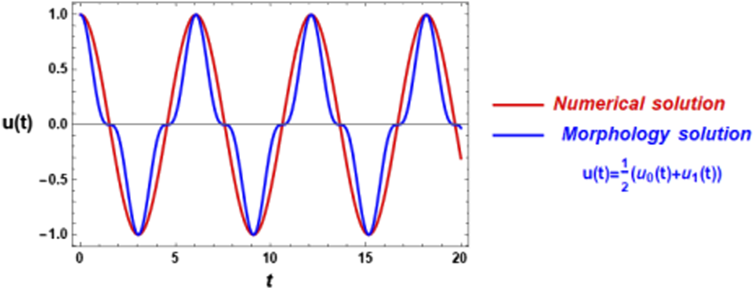
The morphology solution

Since each serial presents an approximate solution individually, then the average between some solutions is called the morphology solution. For example, $u\left(t\right)=\frac{1}{2}\left(u_0\left(t\right)+u_1\left(t\right)\right)$ is a morphology solution composed of the zero-serial solution $u_0\left(t\right)$ and the first-serial successive approximation solution $u_1\left(t\right)$ . Figure 9 illustrates the comparison of the morphology solution $u\left(t\right)=\frac{1}{2}\left(u_0\left(t\right)+u_1\left(t\right)\right)$ with the numerical solution of the Duffing oscillator given by equation (14). It is worthwhile to note that the zero-serial approximate solution has a high agreement with the numerical solution. Nevertheless, there is some deviation observed in Figure 9 between the numerical solution and the morphology solution composed of $u_0\left(t\right)$ and $u_1\left(t\right)$ . This structure led to an improvement in the shape of the apparent oscillation in Figure 2 to come somewhat close to the shape of the numerical solution, but it still needs more subtle improvement.

Figure 9.

Graphical representation of the morphology solution $u\left(t\right)=\frac{1}{2}\left(u_0\left(t\right)+u_1\left(t\right)\right)$ together with the numerical solution. The numerical solution coincides with $u_0\left(t\right)$ the same system as given in Figure 1.

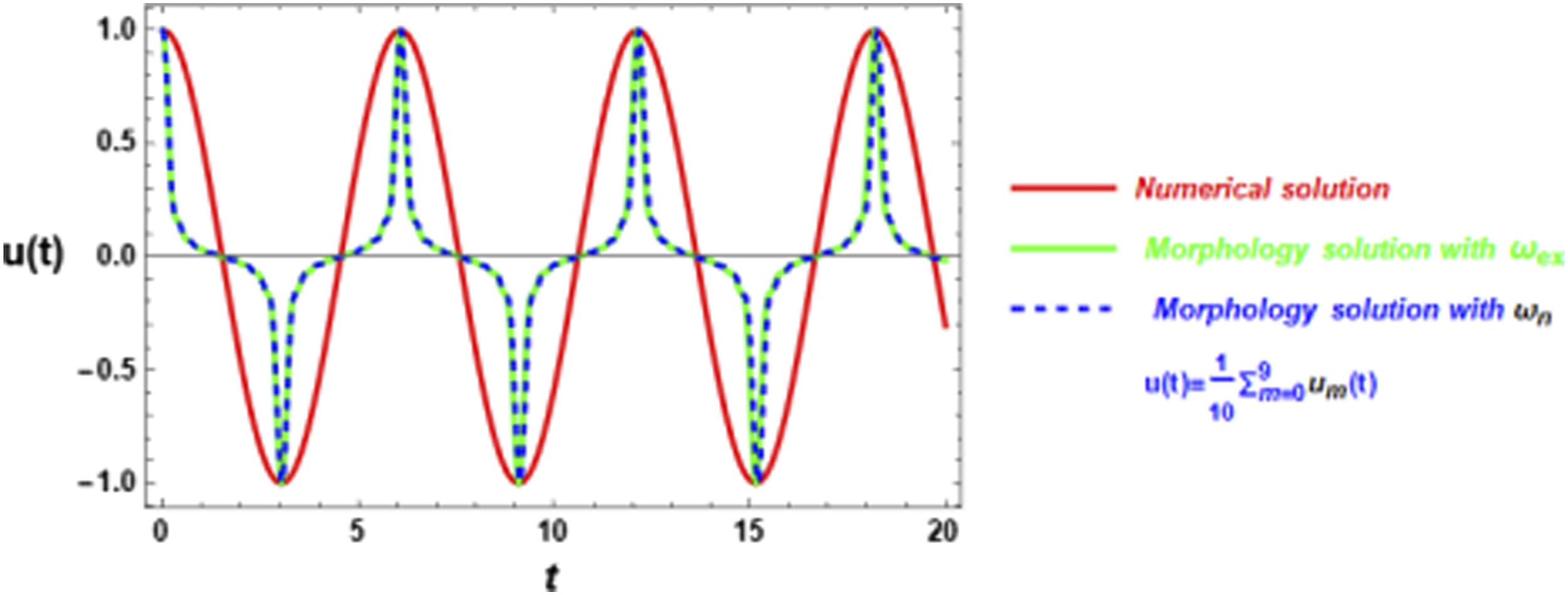
Also, the combination of ten solutions as follows is called the morphology of the ten successive solutions:

$u\left(t\right)={\displaystyle \sum }_{n=0}^9\frac{1}{m}{u}_n\left(t\right);m\ne 0.$

(51)

The above morphology solution has been graphed in Figure 10 for both the exact frequency ${\omega }_{ex}$ and the approximate frequency ${\omega }_n;\hspace{0.17em}n=0,1,2,...,9$ together with the numerical solution for the system considered in Figure 1. It is observed that the formation of ten successive solutions leads to the frame of the volatility shape of the solutions, but at the end, it does not apply to the numerical solution. As shown in Figure 10, there is an excellent agreement between the two morphology curves, but they do not coincide with the numerical solution except at the maximum and lower end points of the oscillation.

Figure 10.

The comparison of the morphology of ten solutions using the exact frequency with the solution using the approximate frequency ${\omega }_n$ and the numerical solution for the same system of Figure 1.

It seems that the morphology solution still requires improvement. For this reason, we must look for a new approach that gives high accuracy compared to the numerical solution. In addition, the new approach must be accurate for large amplitude and not restricted to small ones.

The optimizer of the approximation solutions

In this section, the aim is to obtain an enhanced approximate solution. Firstly, one can assume that the first extended trial solution is set in the form

$U_1\left(t\right)=A\cos {\omega }_{1}t+A\epsilon \left(\cos {\omega }_{1}t-\cos 3{\omega }_{1}t\right).$

(52)

This assumption is similar to that postulated in equation (18), but here, $\left|\epsilon \right|\ll 1$ . The requirements are to determine $\epsilon$ and the unknown frequency ${\omega }_1$ as a function in $\epsilon$ . Substitute the supposed solution (52) back into the efficient formula (13) to get the frequency in the form

${\omega }_1^2\left(\epsilon \right)=\alpha +\frac{1}{4}{A}^{2}Q\left(\frac{3+8\epsilon +18{\epsilon }^2+24{\epsilon }^3+14{\epsilon }^4}{1+2\epsilon +2{\epsilon }^2}\right).$

(53)

It is noted that in the limit as $\epsilon \to 0$ , the above frequency will coincide with the zero-approximate frequency given in (15). The non-zero $\epsilon$ will lead to improving the zero-approximate frequency. The condition of the minimization of ${\omega }_1^2\left(\epsilon \right)$ can be used to determine $\epsilon$ , which requires that

$\frac{d{\omega }_1^2\left(\epsilon \right)}{d\epsilon }=0\hspace{0.17em}.$

(54)

Equation (54) leads to the following equation of the fifth degree in $\epsilon$

$1+12\epsilon +46{\epsilon }^2+76{\epsilon }^3+66{\epsilon }^4+28{\epsilon }^5=0.$

(55)

Keeping in mind that $\left|\epsilon \right|\ll 1$ , so that the higher powers in $\epsilon$ can be canceled from equation (55). Therefore, its solution linearized in $\epsilon$ yields

$\epsilon =-\frac{1}{12}=-0.0833.$

(56)

Substituting back into (53) yields

${\omega }_1^2=\alpha +0.7215A^{2}Q.$

(57)

This is the first correction to the zero-approximate frequency (15). By inserting equations (56) and (57) back into equation (52), the first accurate approximation solution will be performed in the form

$u_1\left(t\right)=\frac{1}{12}A\left(11\cos {\omega }_{1}t+\cos 3{\omega }_{1}t\right).$

(58)

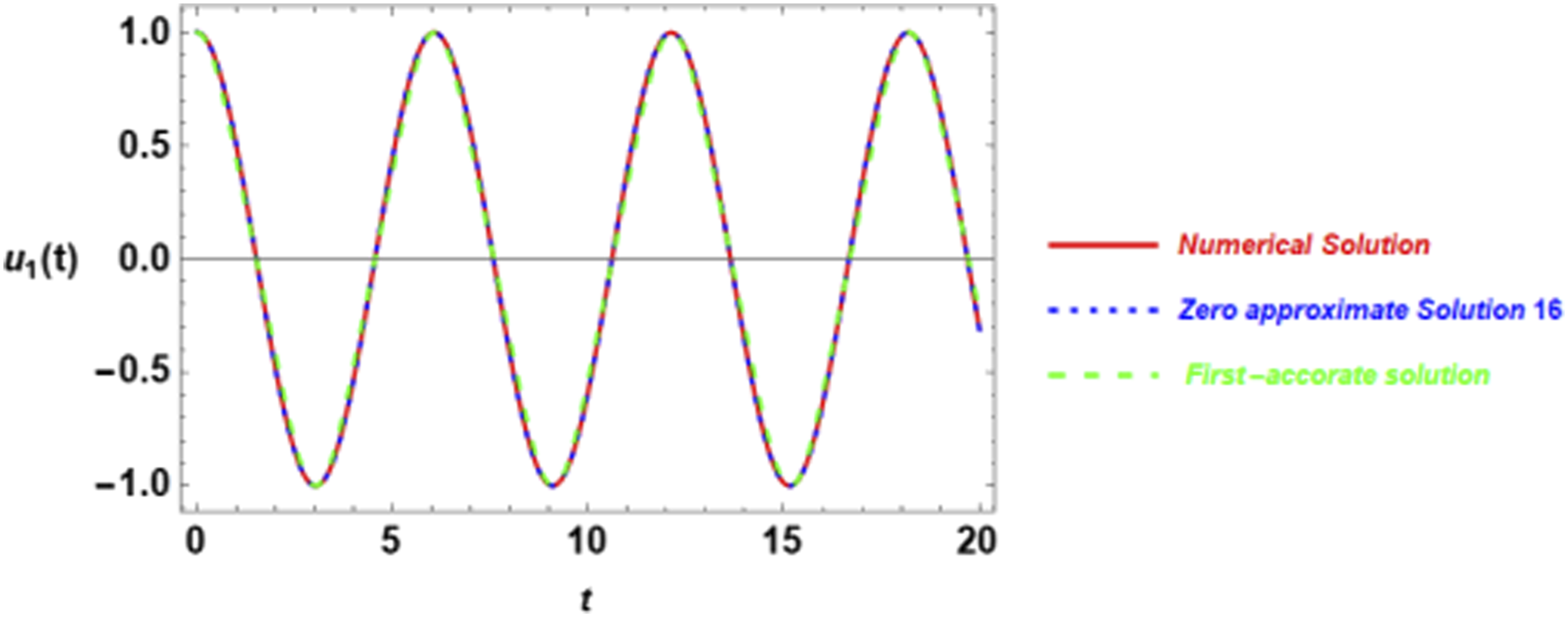
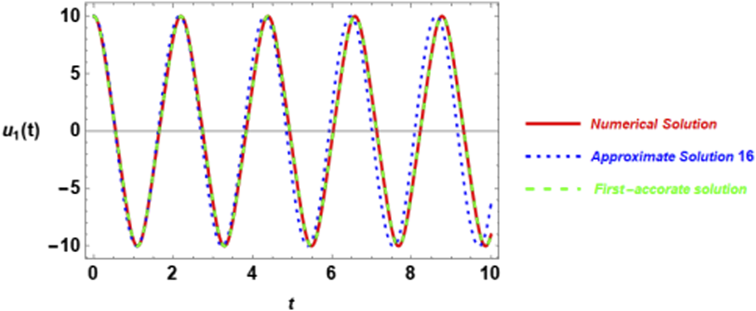
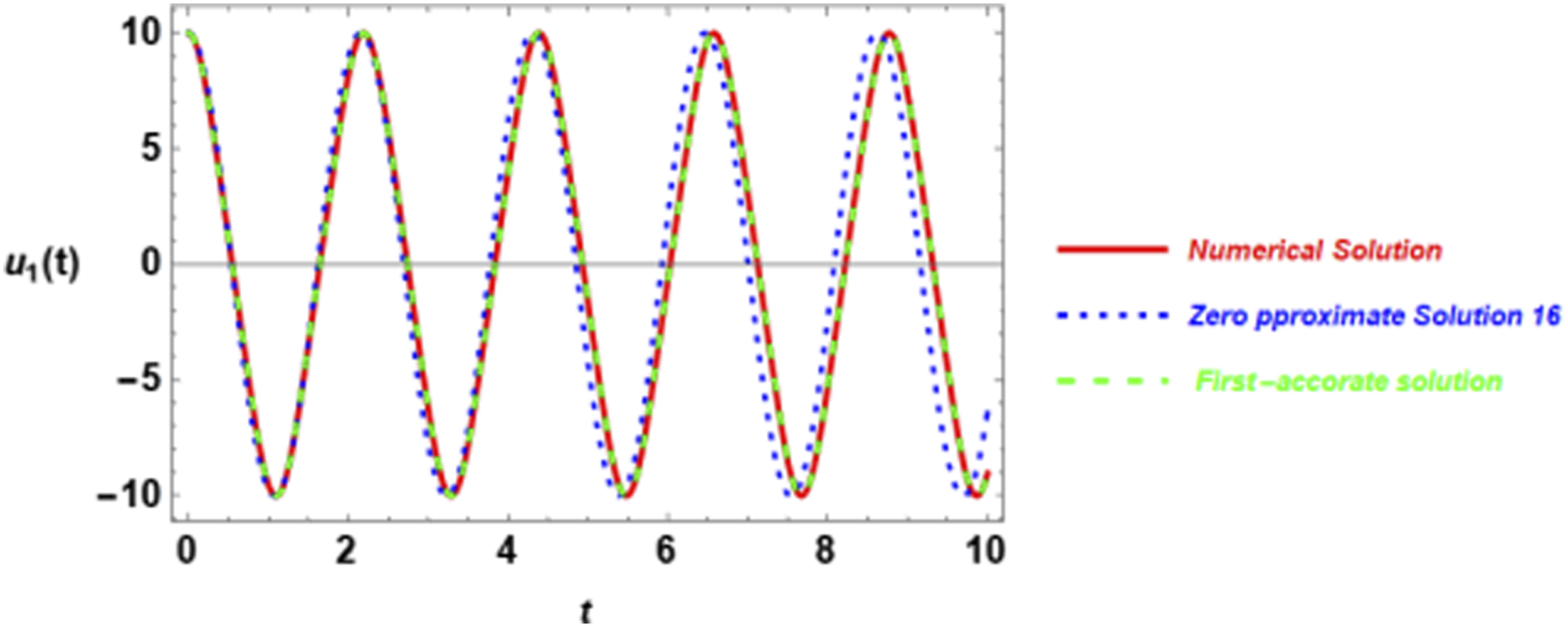
This solution represents the correction of the first-successive solution (29). This solution is illustrated with the comparison of the numerical solution, in Figures 11 and 12, for the amplitudes $A=1$ and amplitude $A=10$ . In these graphs, the zero-approximate (16) is plotted together with the numerical solution and the first accurate (58). It is noted that there is a good agreement between the three solutions for the small amplitude $A=1$ . In the case of $A=10$ , as is shown in Figures 12 and 13, the accurate solution (58) is closer than the numerical solution. This behavior is the advantage of this new approach.

Figure 11.

The comparison of the first accurate with both the zero-order solution (16) and the numerical solution for the system is considered in Figure 1.

Figure 12.

The comparison of the first accurate with both zero-order solution and the numerical solution for large amplitude $A=10$ .

Figure 13.

The comparison of the 10th accurate solution with both zero-order solution (16) and the numerical solution for large amplitude $A=10$ .

The second accurate approximation solution

To enhance the approximate solution, the following second accurate trial solution can be assumed

$U_2\left(t\right)=A\cos {\omega }_{2}t+A\epsilon \left(\cos {\omega }_{2}t-\cos 3{\omega }_{2}t\right)+A{\epsilon }^2\left(\cos {\omega }_{2}t-\cos 5{\omega }_{2}t\right).$

As mentioned before, formula (13) can be used to determine the enhanced frequency ${\omega }_2^2\left(\epsilon \right)$ to be

${\omega }_2^2\left(\epsilon \right)=\alpha +\frac{1}{4}{A}^{2}Q\left(\frac{3+8\epsilon +30{\epsilon }^2+60{\epsilon }^3+92{\epsilon }^4+96{\epsilon }^5+90{\epsilon }^6+44{\epsilon }^7+18{\epsilon }^8}{1+2\epsilon +4{\epsilon }^2+2{\epsilon }^3+2{\epsilon }^4}\right).$

(59)

By linearizing $\epsilon$ , the minimization condition of ${\omega }_2^2\left(\epsilon \right)$ gives the correction for the small parameter $\epsilon$ and the corresponding frequency ${\omega }_2^2$ as

$\epsilon =-\frac{1}{18}=-0.0556,$

(60)

${\omega }_2^2=\alpha +0.7322A^{2}Q.$

(61)

Consequently, the second accurate approximation solution will become in the form

$u_2\left(t\right)=\frac{1}{324}A\left(307\cos {\omega }_{2}t+18\cos 3{\omega }_{2}t-\cos 5{\omega }_{2}t\right).$

(62)

This is the correction to the second successive solution (34). It is easy to continue accumulating the solution to a more correction in the trial solution having the global form

$U_n\left(t\right)=A\cos {\omega }_{n}t+A\left({\displaystyle \sum }_{r=1}^n{\epsilon }^r\hspace{0.17em}\left(\cos {\omega }_{n}t-\cos \left(2r+1\right){\omega }_{n}t\right)\right).$

(63)

Consequently, we have the correction to the third-successive solution (40) in the form

$u_3\left(t\right)=\frac{A}{5832}\left(5525\cos {\omega }_{3}t+324\cos 3{\omega }_{3}t-18\cos 5{\omega }_{3}t+\cos 7{\omega }_{3}t\right),$

(64)

where the correction in the frequency ${\omega }_3^2=\alpha +0.731975A^{2}Q$ occurs at $\epsilon =-0.0556$ .

To tabulate the corrections in the frequency for the serial successive in $n$ , the global trail solution (63) is used and the results are displayed in Table 3. It is observed that the increase in the serial number leads to a slight decrease in the frequency until $n=4$ . The continued increase in $n$ has indicated that the frequency has no additional corrections and is fixed at a constant value.

Table 3.

Illustrate the deviation in the frequency ${\omega }_n^2$ .

The counter $n$	The linearized Solution of $d{\omega }_n^2\left(\epsilon \right)/d\epsilon =0$	Frequency formula for the counter $n$
0	$\epsilon =0$	${\omega }_0^2=\alpha +0.75A^{2}Q$
1	$\epsilon =-\frac{1}{12}$	${\omega }_1^2=\alpha +0.7215A^{2}Q.$
2	$\epsilon =-\frac{1}{18}$	${\omega }_2^2=\alpha +0.732228 A^{2}Q$
3	$\epsilon =-\frac{1}{18}$	${\omega }_3^2=\alpha +0.731975A^{2}Q$
4	$\epsilon =-\frac{1}{18}$	${\omega }_4^2=\alpha +0.731989A^{2}Q$
5	$\epsilon =-\frac{1}{18}$	${\omega }_5^2=\alpha +0.731988A^{2}Q$
6	$\epsilon =-\frac{1}{18}$	${\omega }_6^2=\alpha +0.731988A^{2}Q$
7	$\epsilon =-\frac{1}{18}$	${\omega }_7^2=\alpha +0.731988A^{2}Q$
8	$\epsilon =-\frac{1}{18}$	${\omega }_8^2=\alpha +0.731988A^{2}Q$
9	$\epsilon =-\frac{1}{18}$	${\omega }_9^2=\alpha +0.731988A^{2}Q$
10	$\epsilon =-\frac{1}{18}$	${\omega }_{10}^2=\alpha +0.731988A^{2}Q$

Conclusion

This paper suggests, for the first time, successive approximate solutions of the nonlinear oscillator using the efficient frequency formula. This frequency formula has been performed to work for any successive approximation level. In this proposal, the successive approximate solutions have been derived to a general level with simple approach. The cubic Duffing oscillator is used as an example to show extremely simple calculations and remarkable accuracy. In addition, the higher successive solutions for the Helmholtz–Duffing oscillation have been addressed. The example shows that our result exhibits a perfect agreement with the exact frequency obtained by the elliptic functions. Our approximate frequency has also an extremely high accuracy and simplicity and is better than those obtained by other approaches. Each level of the solution represents, individually, the solution of the nonlinear oscillator. The frequency is estimated at each successive solution. But the obtained solutions have not coincided with the numerical solution. Although the morphology has been a relatively improving solution, more improvements are still required. Finally, we have suggested a new approach to enhancing the approximate solution. This approach has improved the approximate solution and has accounted for large amplitude and able to satisfy large amplitude. It can be used as a paradigm for many other applications, with each kind of solving process.