This article investigates the impact of three harmonically external moments on the motion of a four-degrees-of-freedom (DOF) nonlinear dynamical system composed of a double rigid pendulum connected to a nonlinear spring with linear damping. In light of the system’s generalized coordinates, the governing system (GS) of motion is derived using Lagrange’s equations. With the use of the multiple-scales method (MSM), the approximate solutions (AS) of the equations of this system are obtained up to a higher order of approximation, maybe the third order. Within the framework of the absence of secular terms, the conditions of solvability are obtained. Accordingly, the different resonance cases are categorized, and three of them are investigated simultaneously. Thus, these conditions are updated in preparation for achieving the modulation equations (ME) for the examined system. The numerical solutions (NS) of the GS are achieved using the algorithms of fourth-order Runge–Kutta (4RK), which are compared with the AS, which displays their high degree of consistency and demonstrates the precision of the MSM. The motion’s time history, steady-state solutions, and resonance curves are graphed to demonstrate the influence of various system physical parameters. All relevant fixed points at steady-state situations are identified and graphed in accordance with the Routh–Hurwitz criteria (RHC). Therefore, the zones of stability/instability of are checked and analyzed. Numerous real-world applications in disciplines like engineering and physics attest to the significance of the nonlinear dynamical system under study such as in shipbuilding, automotive devices, structure vibration, developing robots, and analysis of human walking.
Mathematicians, physicists, biologists, engineers, and other researchers are interested in nonlinear problems because most dynamical systems in nature are nonlinear, in which they reflect time-dependent variables.1 Compared to linear systems, these can seem chaotic, counterintuitive, or unexpected. These mechanisms could involve the movement of a clock or the flow of water through a conduit. Nonlinear unpredictable behavior is common in engineering machinery, rotor dynamics, compressors, pumps compressors, and transportation equipment, to name just a few examples of nonlinear dynamics’ applications.2–4 There are difficult-to-find solutions for such complex systems. Thus, perturbation methods can be used to estimate the behavior of dynamical systems, in which the scientific community uses sophisticated of these methods; like the MSM to examine such systems.5,6
According to dual-phase lagging, the authors of Reference 7 generalized thermo-elasticity theory for the thermo-elastic damping of a tiny rotating ring. The strain’s theory of thermo-elasticity fractional-order is used to describe the vibration of a gold nano-beam in many publications, including,8,9 within the context of Caputo–Fabrizio’s.10 Numerical results are achieved and graphically portrayed in accordance with the various values of electrical voltage and resistivity.
The author of Reference 11 investigated how the vibrations of charged particles, caused by the Larmor rotation1 of those particles, cause a resonance, and how that resonance is responsible for the force under consideration. The pendulum under periodic external perturbation is the simplest model studied in Reference 12. Nonlinear oscillations around a resonance are analyzed to determine their behavior. For further information on how resonances affect dynamical systems, see Reference 13. In References 14–17, the authors looked into different kinds of pendulums, from the most basic pendulum with a rigid arm to a more complex one with an elastic arm. They used the MSM, which involves solving the GS of motion on several scales, to get close. As a result, they are concerned about the reliability of the motion control system.
Interpolated mapping18 and numerical methods19 were used to establish the global domains of attraction and examine the determinants of stability in a linear spring-pendulum system.17 Both robust sliding mode and optimal polynomial controls were used by the author to keep the Duffing oscillators under check in Reference 20. The behavior of an excited spring pendulum with a freely revolving pivot point using the MSM was investigated in Reference 21. The solutions were able to achieve up to third-order autonomy for the studied system. The system exhibits a chain of double bifurcations in period, a feature characteristic of chaotic dynamics. Mathematical pendulums with vertical and horizontal oscillations near their pivot were studied in Reference 22, specifically the problem of their planar rotating motion. In this way, the AS were discovered, and the original system's stability was verified because the trajectory of the supported point exhibits an elliptic form close to a circle. The relative periodic motion of a rigid body (RB) strung on an elastic thread in the vertical plane was studied in Reference 23. The analytical solutions to the GS of motion were obtained using the small parameter method.5 Using the 4RK,19 the NS to this problem were investigated in Reference 24.
The swing of a pendulum with several DOF, where the pivot point follows a Lissajous curve was studied in Reference 25, in which the potential resonance scenarios were obtained. The issue of moving pivot point of a damped pendulum along an ellipse, was examined from different angles in Reference 26. Using the same technique, the ME were extracted and all steady-state solutions have been found. Time history diagrams are used to display the gained solutions, and phase plane projections were provided to examine the model’s dynamical behavior. Some limited cases were investigated when the movement of the suspension point was on a circular trajectory,27 or when it was considered to be fixed.28 Following up on their earlier work in Reference 25, the authors continued their investigation of a dynamical system with 3DOF in Reference 29. They thought about a pendulum of a damped spring linked with a RB from its free end. Using the MSM, AS were obtained and the multiple resonance cases were examined. Nonlinear vibrations of the axially accelerated spring issue were studied in Reference 30. The GS of motion was derived using the Hamiltonian concept and then solved using the same approach. Contrarily, in Reference 31, the Hamiltonian technique was used to study the planar vibrations of the simple pendulum. In Reference 32, the time-optimal trajectory of a trolley was determined by studying a dynamical model of a double pendulum coupled to a moving trolley. The movement of a stimulated spring pendulum attached to a RB was analyzed in Reference 33. It was supposed that the pendulum’s supported point could only swing in an elliptical route with a stationary angular velocity. The main case of external resonance was examined.
The problem of an auto-parametric vibrating system, which involves two nonlinearly coupled subsystems, is crucial. The first subsystem can be attached to an absorber, and it was activated by an external harmonic force, while the major one reduces the response of the first subsystem.34–40 A nonlinear damping 2DOF dynamical model of a connected spring with a vibrating system was examined in Reference 37, while a 4DOF auto-parametric pendulum linked to a RB was investigated in Reference 38. In Reference 39, the authors investigated computationally and empirically the auto-parametric system dynamic response to kinematic excitation. Plots were used to test the system’s regularity. The behavior of a pendulum absorber coupled to a damped oscillatory system as an auto-parametric system is analyzed in Reference 40. The harmonic balance technique,5 was used to obtain the AS close to resonance. In Reference 41, an auto-parametric damped Duffing system coupled with an excited pendulum was examined using the MSM to obtain the resonance requirements. However, the solution of two coupled mass springs was obtained using this method, and new excitation conditions in the presence of auto-parametric resonance were discussed in Reference 42. In Reference 43, the authors shed their attention on the resonance of an auto-parametric vibrating system with a third-order nonlinearity. A similar system under external influences was studied to examine its bifurcation and stability in Reference 44 and Reference 45.
Homotopy perturbation method (HPM) was proposed in several scientific works, for example, References 46, 47 and it is frequently used to solve the problems of nonlinear oscillations with microsystems oscillators.47–49 On the other hand, a modification of HPM is used in Reference 46 to obtain the analytic solution of a magnetic inverted pendulum. Some of the emerging resonance cases are investigated in light of the MSM procedure. The solutions of conservative nonlinear oscillators and micro-electromechanical systems are presented in References 47–49 using the modification of HPM. For more information about the solutions of nonlinear oscillators, dynamical systems, and the stability of such systems, see References 50–55.
The motion of 2DOF dynamical systems, which are formed by two RB pendulums with embedded magnets in a dynamic magnetic field, was examined numerically and experimentally in References 56,57 in which these systems defend unpredictable and predictable motion. Phase sketches, time series, bifurcation, and Poincaré maps were examined in view of the system’s nonlinear dynamics. The analytic approximations were unable to be found, since perturbation strategies were difficult to utilize. The MSM was used to estimate solutions of a damped elastic RB pendulum with linear stiffness in Reference 29. In Reference 58, the pendulum’s motion with a relocating suspension point along an elliptical path was examined, in which the spring’s stiffness was assumed to be linear. In Reference 59, the authors studied the nonlinear behavior of an elastically damped RB pendulum when its pivot point follows a Lissajous pattern. The analytical asymptotic solutions were verified by comparing them with numerical results. In Reference 60, the motion of a 3DOF triple pendulum in a plane was checked, taking into account the case of a fixed suspension point. The solvable criteria of steady-state solutions are assessed and discussed. The nonlinear movement of the 3DOF pendulum model was examined in Reference 61 in light of the motion of its suspension point on a Lissajous trajectory. By categorizing resonance cases and assessing the prerequisites for the solvability of the ME, the asymptotic approximation solutions were generated. In Reference 62, the authors used an energy harvesting device to transform the vibrational motion of a spring pendulum into electric energy. Another dynamical system with 6DOF can be found in Reference 63, in which it is solved according to the restrictions of Bobylev–Steklov.
This study investigates the impact of harmonically external moments on the oscillation of a dynamical system consisting of a double rigid body pendulum connected to a nonlinear damped spring. In light of the system’s generalized coordinates, the GS of motion is derived using Lagrange’s equations and solved analytically using MSM up to a higher order of approximation. The requirements of solvability are obtained in the context of the absence of secular terms. Therefore, various resonance cases are categorized accordingly, and four of them are analyzed simultaneously. To achieve the ME for the system under consideration, these criteria were amended. The 4RK is used to generate the NS for the GS, which are then compared with the AS to show their high degree of consistency and highlight the accuracy of the MSM. The motion’s temporal history, steady-state solutions, and resonance curves are used to graphically demonstrate the influence of various system physical factors. According to the RHC, all significant fixed points at steady-state conditions are identified and plotted. As a result, the regions of stability and instability are verified and assessed. The studied model is helpful in many areas of physics and engineering that involve vibration systems, including building vibrations, assessments of human or robotic walking, transportation systems, shipbuilding, and ship motion.
Description of the dynamical system
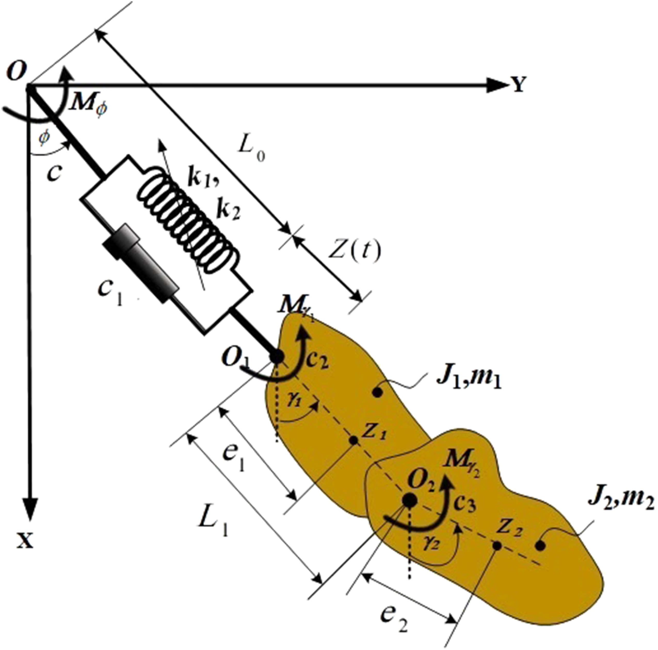
This section examines a 4DOF planar motion of a coupled nonlinear damped spring with two rigid bodies with masses and from its end point , while the other end is considered to be a fixed origin of the Cartesian coordinates system . It must be mentioned that both bodies are linked together at the point , while the spring has a length at rest and exhibits linear and cubic nonlinearity, respectively, with stiffness coefficients and , see Figure 1. The rotation angles at and are and , respectively. The quantities and represent the distance between the gravity centers of bodies and the rotational centers , and the link length of the first body, respectively. Moreover, the bodies moments of inertia for the masses relative to (perpendicular to the plane ) are symbolized by . Let us consider the action of external harmonic excitation moments and (where and are the frequencies and amplitudes of the acted moments), at the points and , respectively. Moreover, we suppose that the resistance moments at have coefficients and of viscous damping. Therefore, the viscous forces due to the applied moments and spring damping are and .
Visualizes dynamical motion.
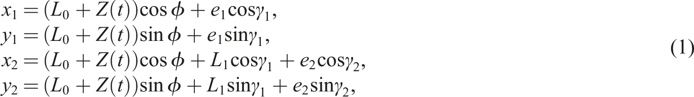
After understanding the aforementioned description of the investigated system, one can write the coordinates and of the points as follows
where is the normal length of the spring and is the elongation of the spring after time .
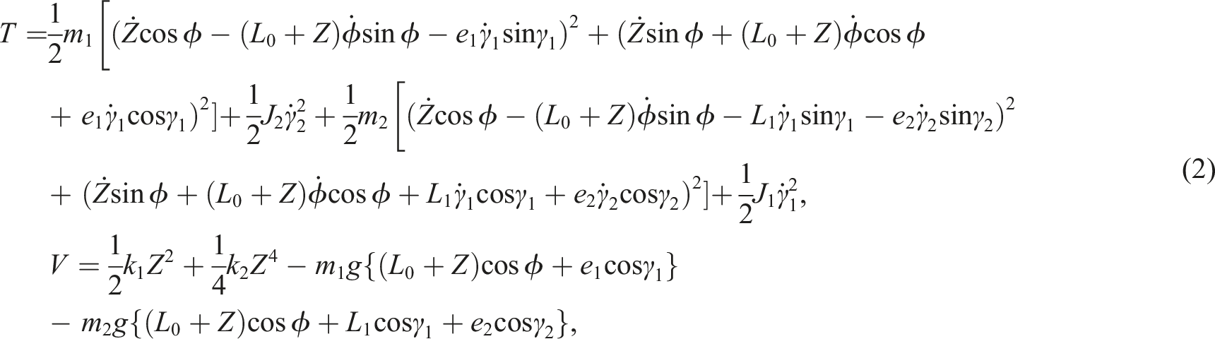
The kinetic and potential energies and of the system are shown below
where dots are the differentiation regarding time and is the gravitational acceleration.
Let denotes static elongation at the position of steady state. Therefore, we can write
As a result of the system generalized coordinates , one can calculate Lagrange’s function , and then the GS of motion can be obtained by utilizing the below Lagrange’s equations
where are the generalized velocities of the examined system and the corresponding forces of the coordinates are
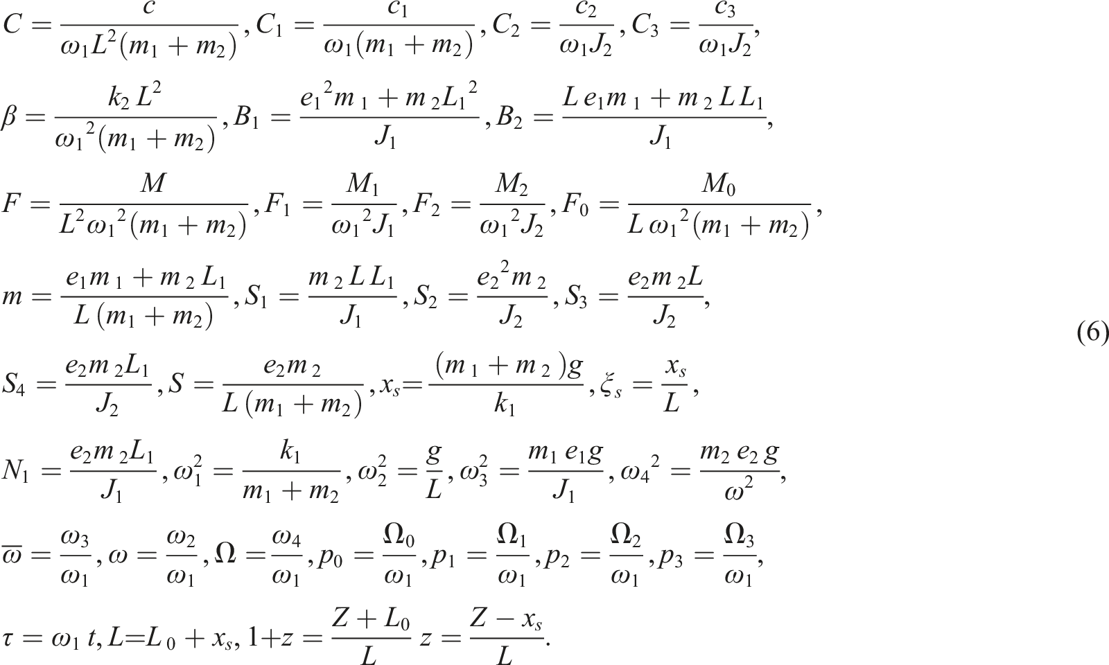
It must be mentioned that dimensionless nature of the coordinates, parameters, frequencies, and time can help us handle the dynamical system easier. Therefore, the below dimensionless parameters are used
Moreover, the dimensionless condition of (3) has the form
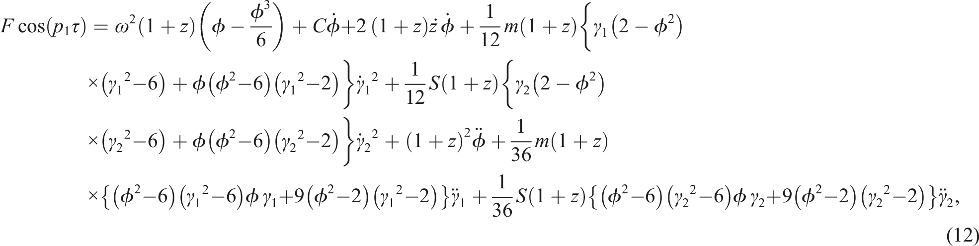
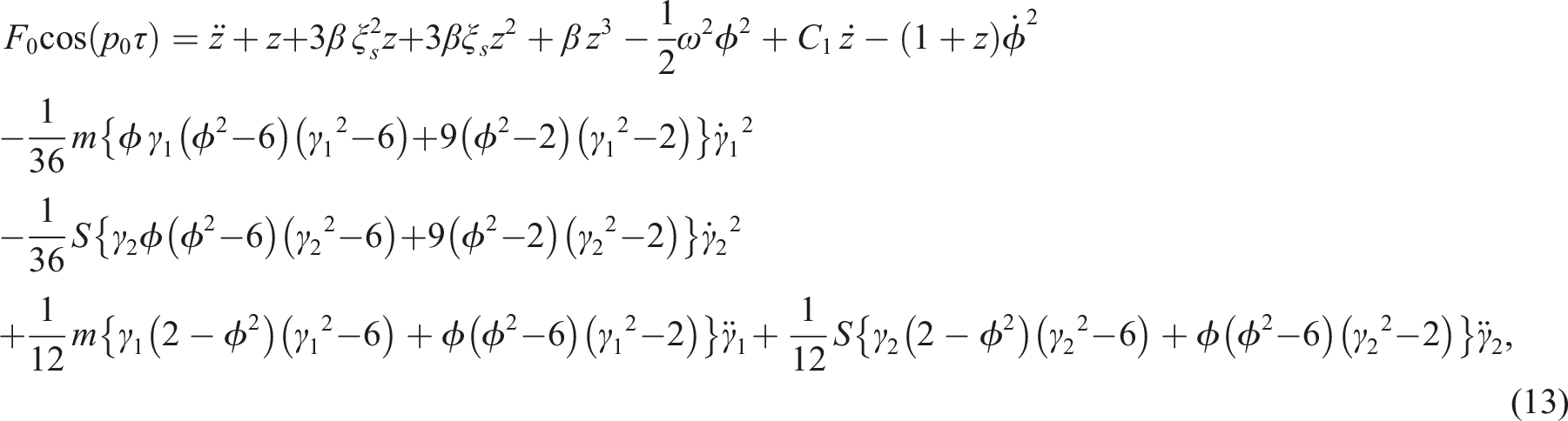
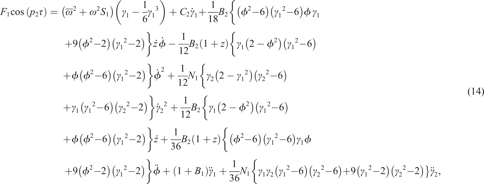
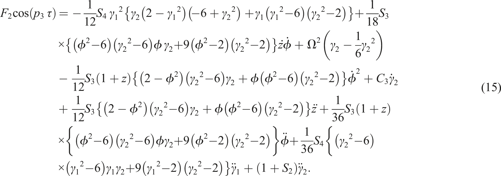
Making use of (2), (5), (6), and (7) into (4) to obtain the required GS of equations of motion as follows
The above-mentioned GS of equations (8)–(11) consists of four nonlinear ordinary differential equations (ODE) regarding and . A closer look at these equations shows that they are coupled, and they contain two second-order derivatives of or more from the required variables, besides the first derivatives of all variables, which is difficult but not impossible to deal with. Therefore, the following section presents the AS of these equations using a suitable perturbation approach.
The perturbation methodology
The objective of this section is to utilize the MSM in order to obtain the AS of the equations (8)–(11) up to the third order and to establish the criteria for solvability in view of the arising resonance cases. This goal can be accomplished by approximating the trigonometric functions in (8)–(11) up to the third order in the proximity location of static equilibrium. In light of these notes, equations (8)–(11) can be reformulated as follows
It’s important to understand that the vibration amplitudes, in particular the generalized coordinates, must be expressed in terms of a small parameter . As a result, the new variables and can be considered as follows
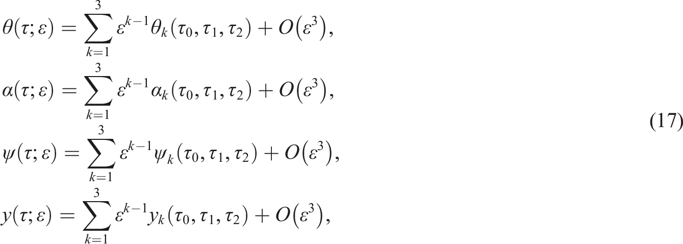
Based on the MSM procedure,5,6 we can express these variables as a form of power series of as follows
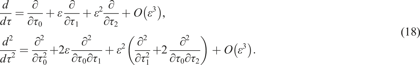
where are distinct time scales, in which they reflect the meaning of fast and slow time scales as and , respectively. Hence, the time derivatives relating to can be adjusted to and by using the following chain rule
It is observed that terms like and higher have been overlooked due to their minimal values.
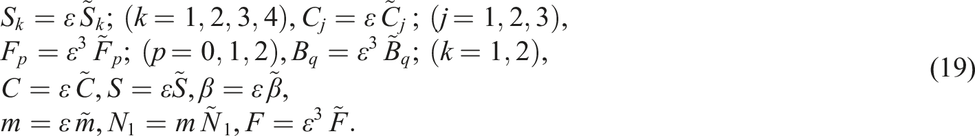
Considering the smallness of the parameters and according to
where and are parameters of order unity.
Three groups of partial differential equations (PDE) can be obtained after substituting (16)–(19) into (12)–(15) and equating coefficients of the same powers of , in which each group contains four PDE from second order and they have the forms
Order of
Order of
Order of
It is crucial to note that the above-mentioned groups of PDE can be solved subsequently in the order they were presented. As a result, the generic solutions of equations (20)–(23) can be expressed as follows
where and represent undetermined complex functions and complex conjugates.
Making use of the solutions (32)–(35) into the PDE (24)–(27) and then removing terms that yield secular ones to obtain the following removal conditions
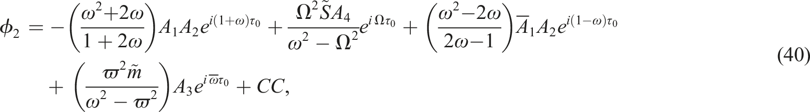
As a consequence, the solutions of second-order can be written as follows
where are the former terms complex conjugates.
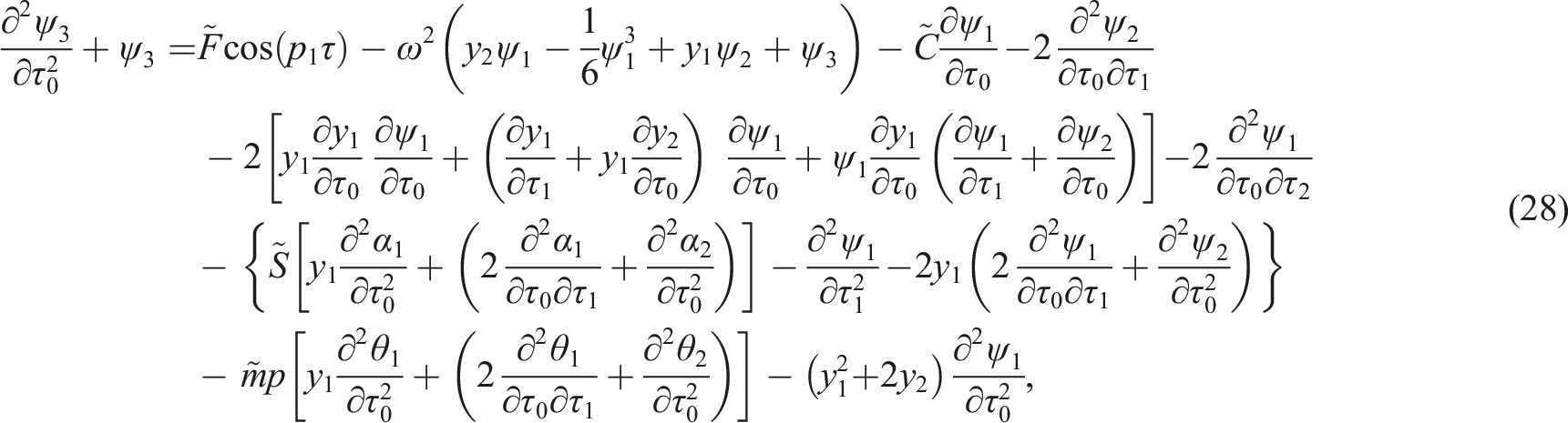
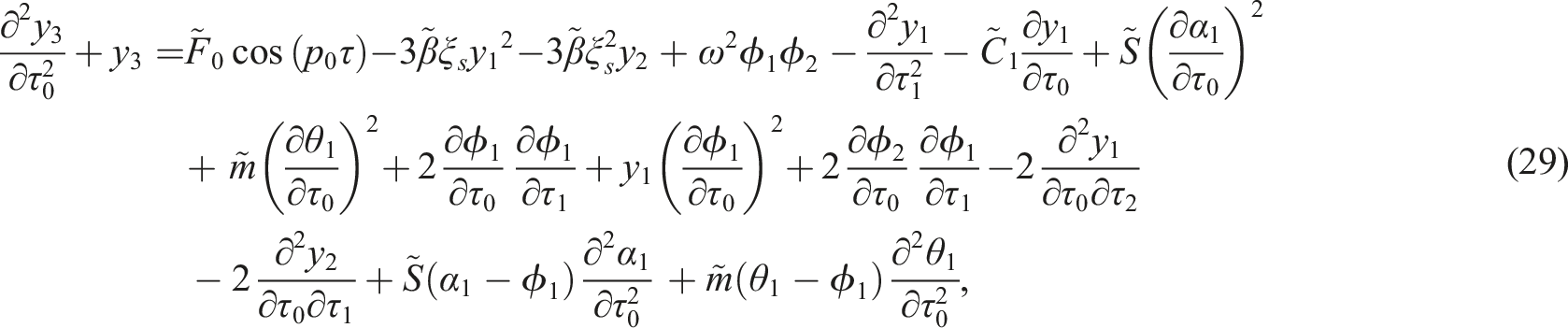
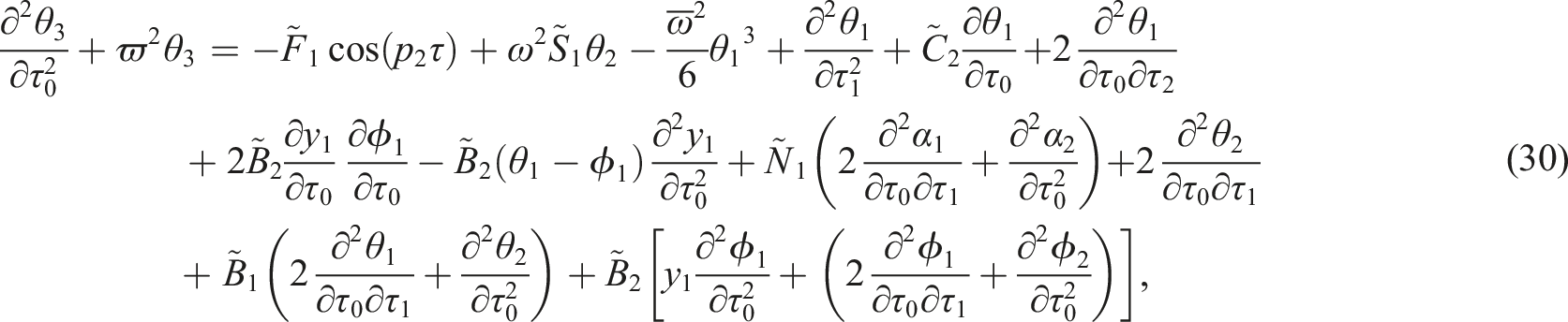
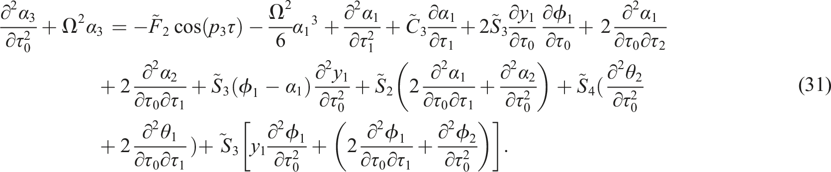
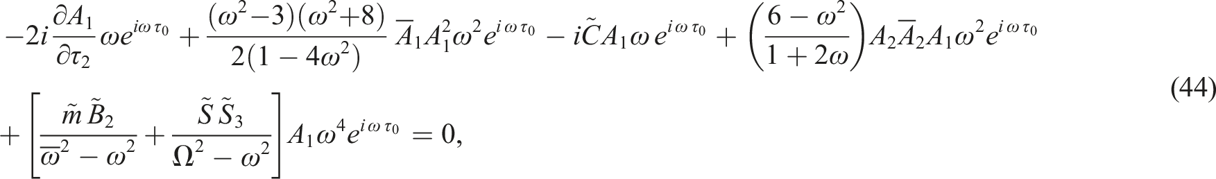
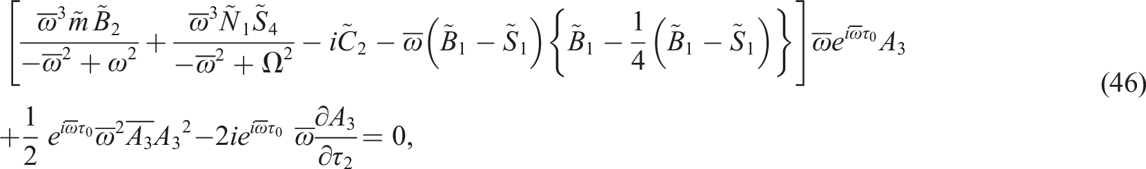
One may determine the conditions for excluding secular terms from the approximation of order three by substituting the preceding solutions (32)–(35) and (40)–(43) into (28)–(31) to get
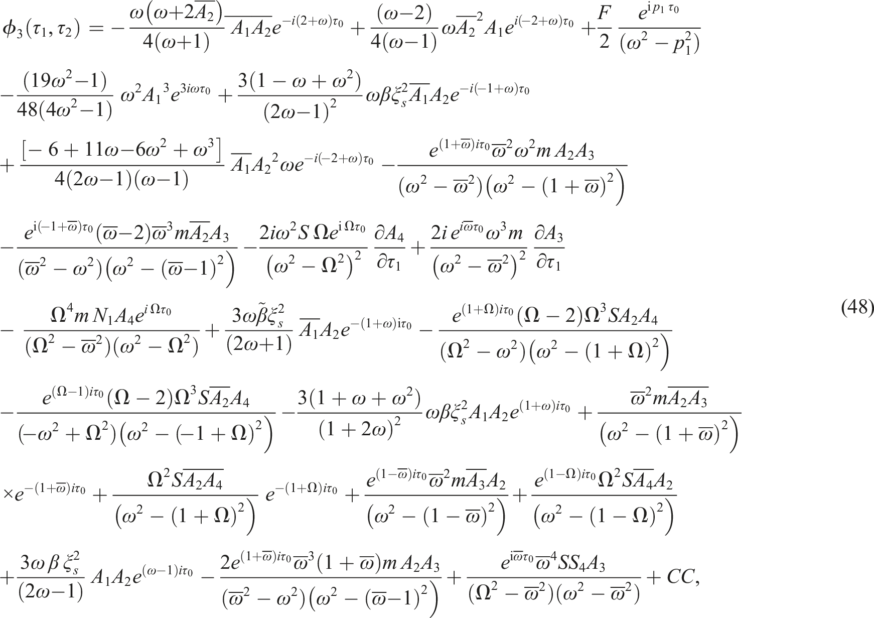
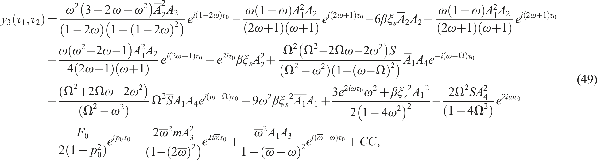
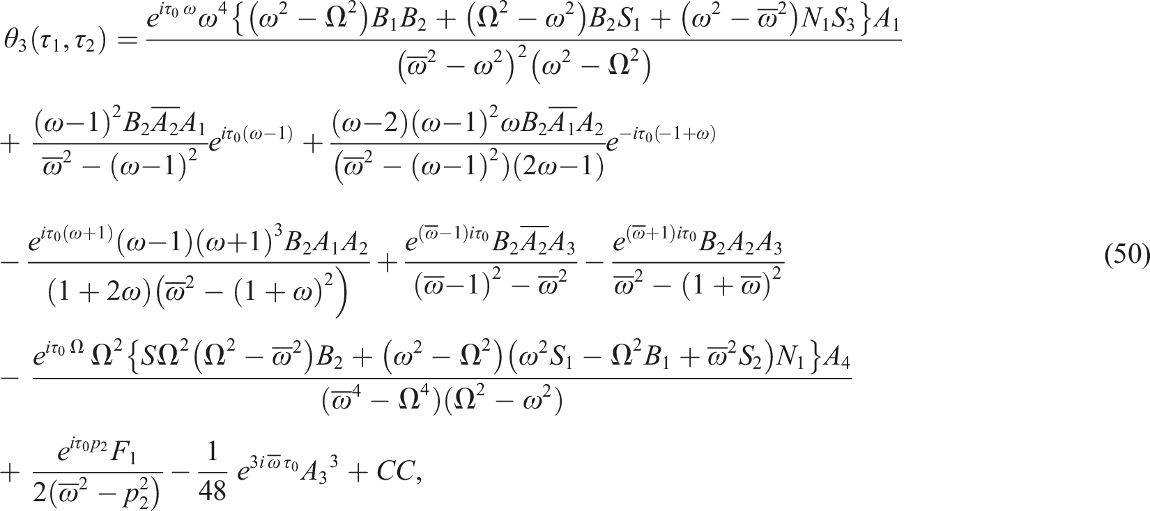
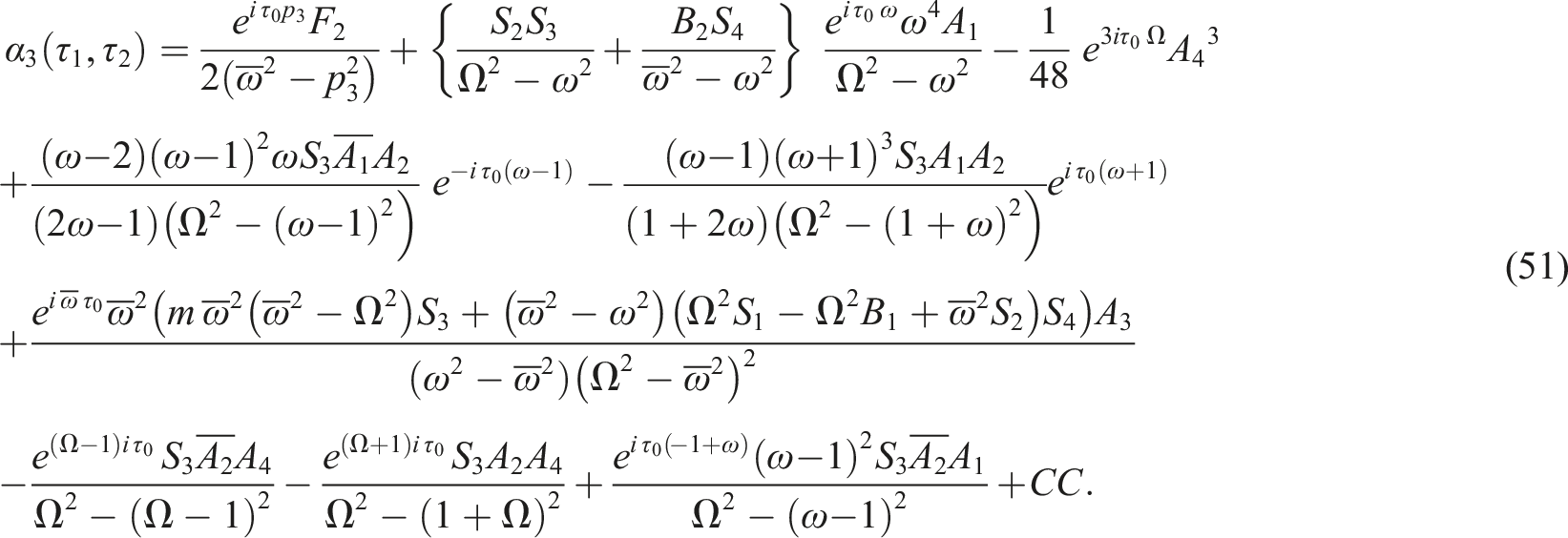
These constraints allow us to express the third-order approximations in the forms
By examining conditions (36)–(39) and (44)–(47), the unidentified functions can be determined. Substituting the above solutions of first, second, and third order into series (17), and then using (16) to obtain the desired AS up to the third-order of approximation.
As already mentioned, dealing with the AMM requires the use of an infinite number of different time scales instead of just one time variable. The proper penalty for this flexibility is thought to be the solvability requirements, which entail the elimination of secular parts from fast time variables. The fast scales impose restrictions on the structure of the projected solutions. Furthermore, it is essential to confirm that the conditions of solvability for various orders are consistent. These conditions place restrictions on the amplitudes of “free” resonant cases that appear in each order of expansion. Inaccurate outcomes from the analysis or just allowing simple solutions are possible if the constraints are not met. It should be recognized that alternative free amplitude possibilities may produce results that are in conflict with each other.64
Resonance classification and modulation equations
The classification of resonance scenarios that could appear in second or third-order solutions, along with the analysis of four of them, are both crucial elements of this section. These scenarios are known to happen when the denominators of the mentioned orders of solutions converge to zero.60,65 Thus, it could possibly be classified as
(i) At and , the first scenario that is known by primary external resonance is obtained.
(ii) At and , the second scenario, known by internal resonance, has occurred.
The examined system will behave poorly if one of the resonance situations is met. Therefore, we will adjust the used method of perturbation. Moreover, the strategy outlined above is still applicable if the vibrations have values different from the resonance. To address this problem, we will look into the four primary external resonances that occur simultaneously.
These expressions show the relative proximity of and to and , respectively.
To achieve this goal, it is essential to use the following dimensionless detuning parameters that measure how far the vibrations are from the stern resonance. Afterwards, one can write
Once this is done, we can represent these parameters in terms of in accordance with the following
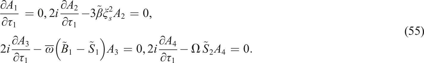
In order to obtain the following solvability requirements, substituting (51) and (52) into PDE (24)–(31) and then eliminating the terms that generate secular ones
For the fourth second-order equations
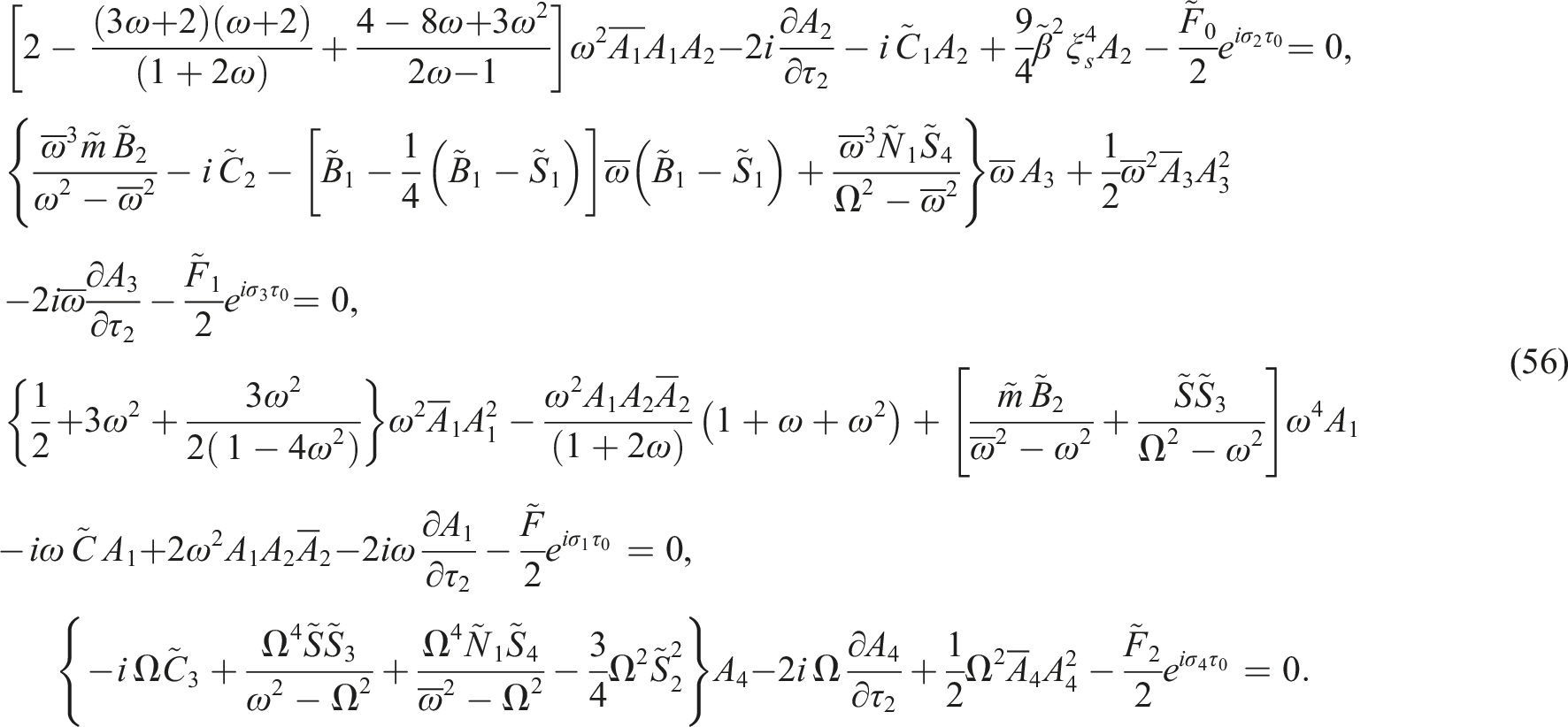
Criteria of third-order approximation
It should be emphasized that the aforementioned criteria (55) and (56) reveal the functions depend on the fast time scales and , in which it can be evaluated from these criteria. Therefore, we can express them in the following polar forms
where and are assumed to be real functions, and they represent the amplitudes and phases of the solutions and .
Take into account the adjusted phases that are listed below
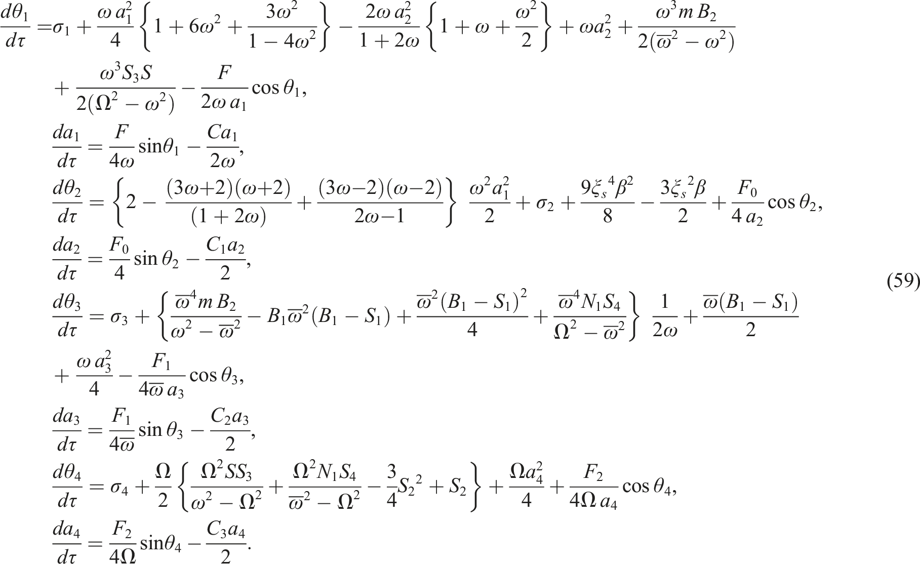
The preceding PDE of solvability criteria (55) and (56) can be transformed into ODE by substituting (57) and (58) into (55) and (56). Then separating the real and imaginary parts to obtain eight ODE of first-order, in which they are known by the ME of the examined system at the same time, considering simultaneously resonances
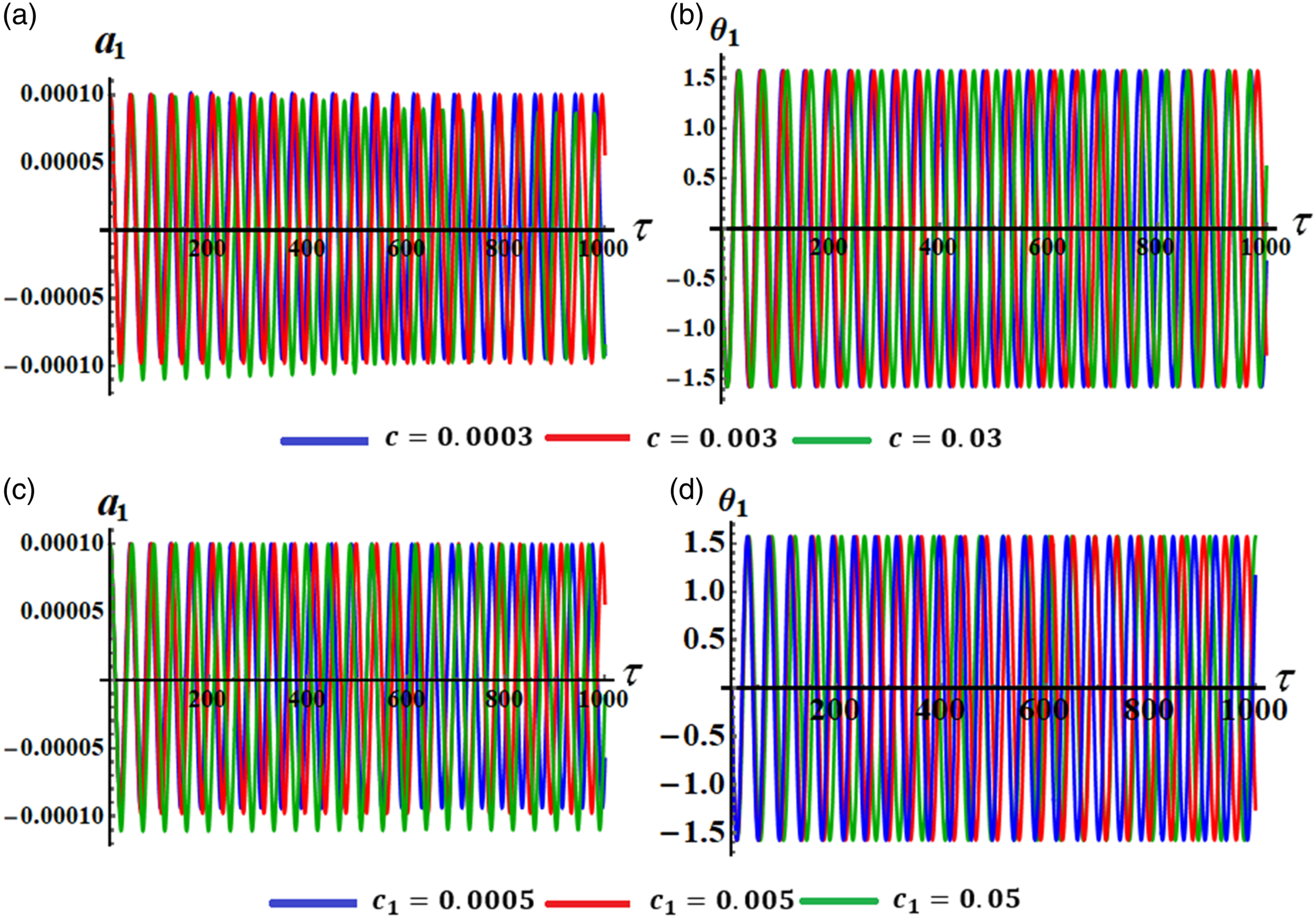
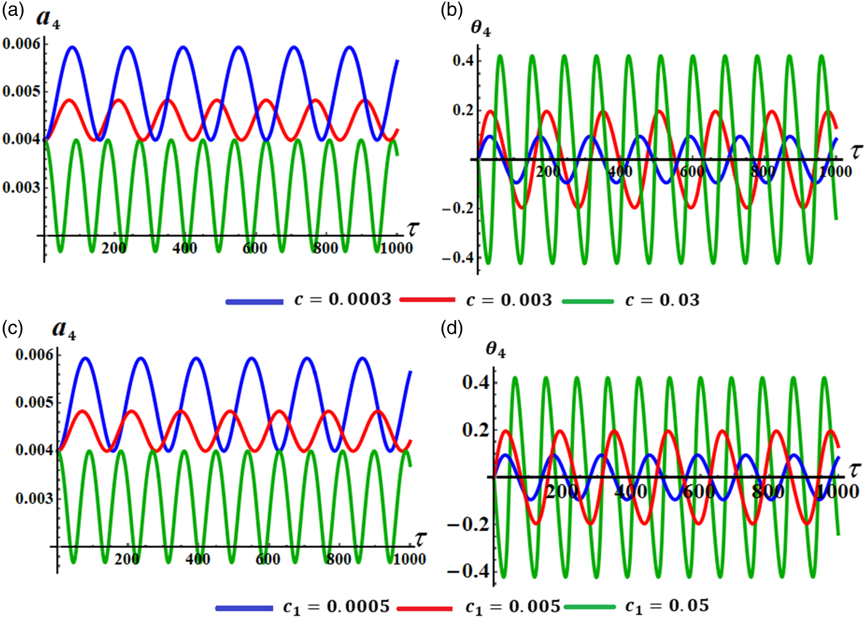
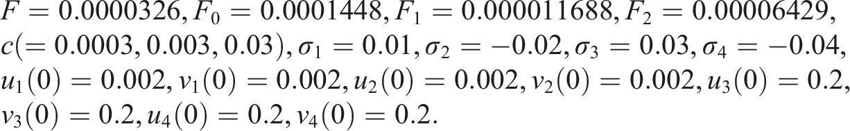
With reference to system (59), the time histories of its numerical solutions and are graphed in Figures 2–5. These figures are computed using different values of and when in addition to the following data60
Describes the behavior of the solutions: (a) at various values of , (b) at various values of , (c) at various values of , (b) at various values of .
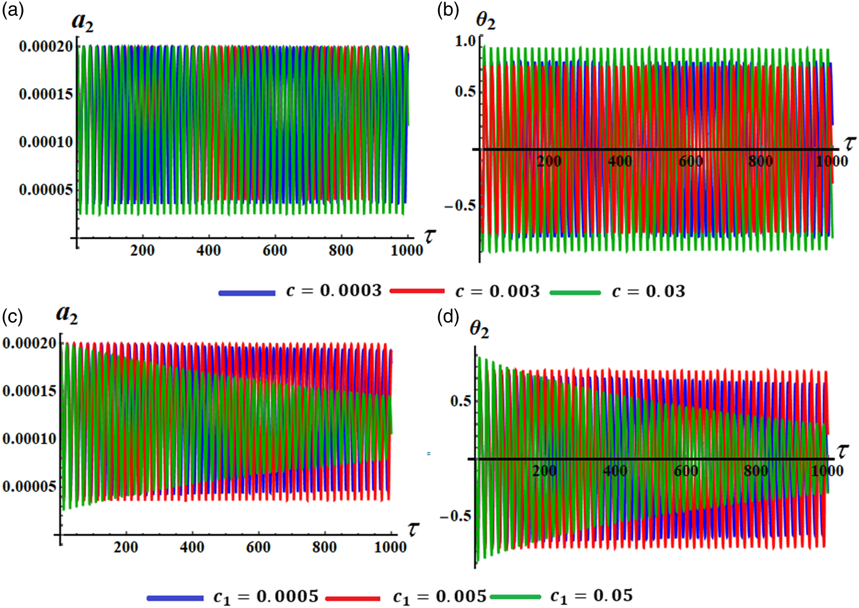
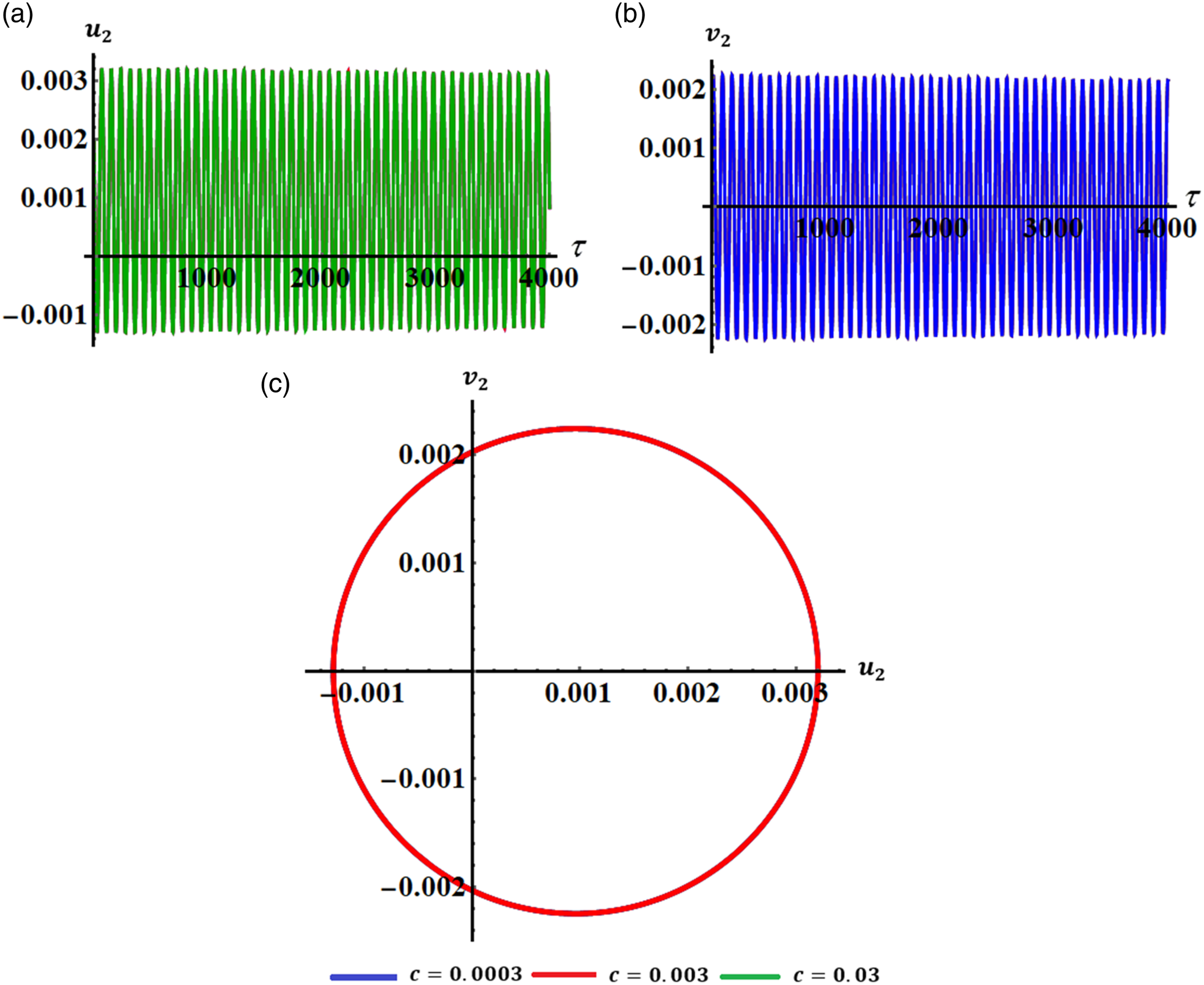
Explores the behavior of the solutions: (a) at various values of , (b) at various values of , (c) at various values of , (b) at various values of .
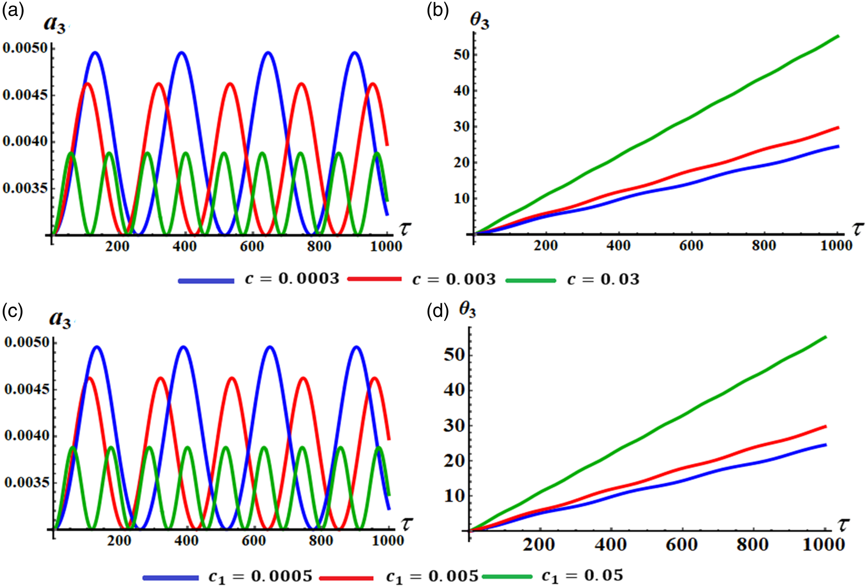
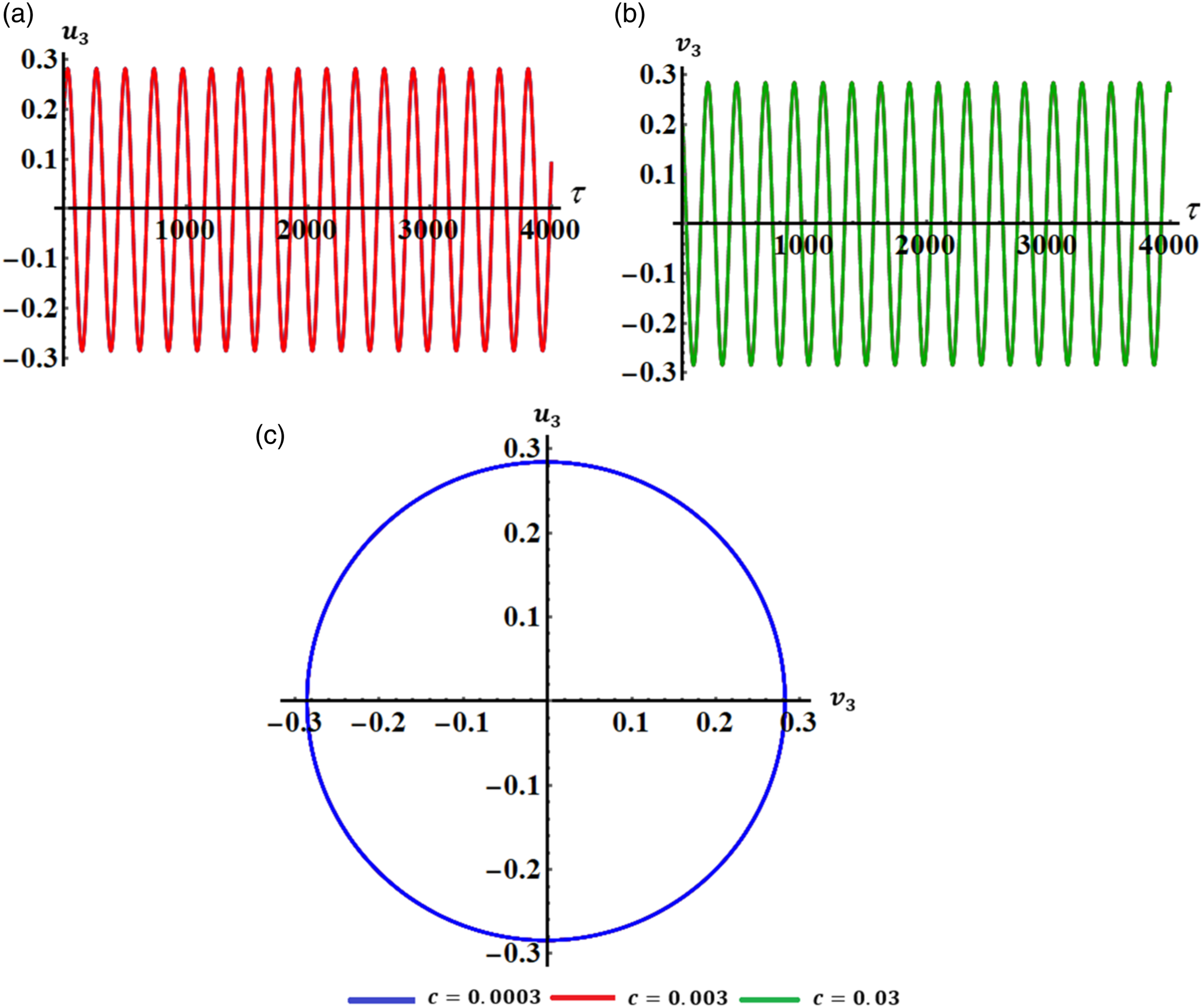
Reveals the behavior of the solutions: (a) at various values of , (b) at various values of , (c) at various values of , (b) at various values of .
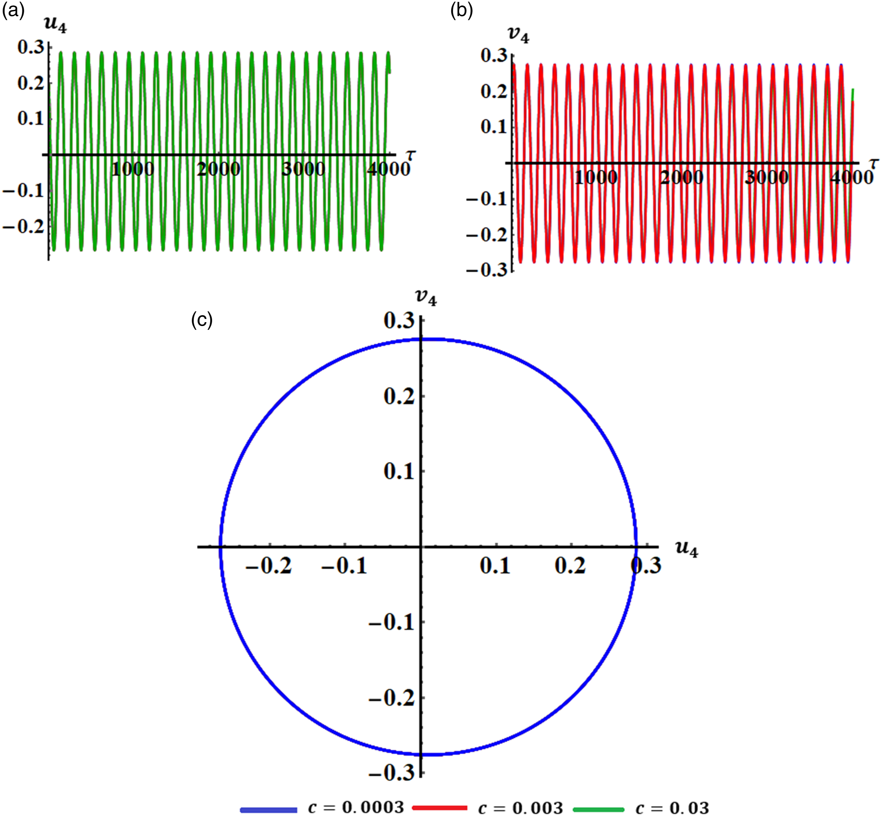
Represents the behavior of the solutions: (a) at various values of , (b) at various values of , (c) at various values of , (b) at various values of .
The curves of Figures 2 and 3 explore the variation of the numerical results of amplitudes and adjusted phases via dimensionless time at various values of the damping parameters and . It is noted that the plotted waves describing these parameters have the form of periodic forms, in which the amplitudes of these waves decrease with the increase of values, as seen in Figure 2(a). It is observed in this part that a decay behavior of the wave at . On the other hand, there is no change of the amplitudes of the waves illustrating , as drawn in Figure 2(b). The behavior of has a periodic manner with the change of values, as graphed in Figure 2(c). An increase in the amplitude is observed with increasing of values, while no variation is seen for the curves of Figure 2(d). The examination of the drawn curves in parts of Figure 3 reveals that all curves have periodic behavior with the change of or even with , except for the wave that describe the behavior of at , it has a decay behavior, as seen in Figure 3(c). The reason for this is due to the mathematical structure of the equations of the system (59). Accordingly, it becomes clear to us that if the behavior is periodic or decaying, the behavior of the solution is stable.
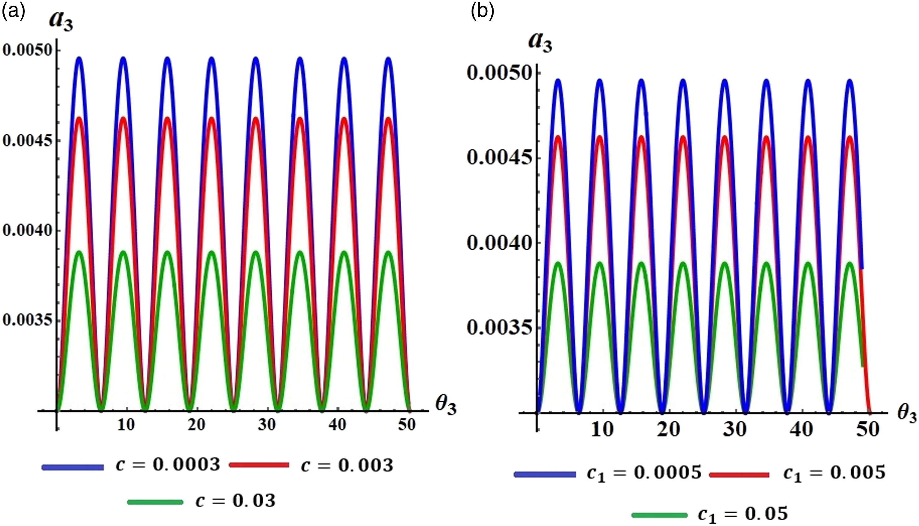
The inspection of parts of Figures 4 and 5, shows the waves behavior of the amplitudes and adjusted phases during the interval with the change of the values of and . It must be mentioned that the drawn curves of have periodic forms, in which the amplitudes of the waves represented by these curves decrease with the increase of and , while their oscillation number increases along with the decreasing of their wavelengths, as seen in in Figures 4(a) and (c). On the other side, the behavior of increases gradually over entire time interval, as indicated in Figures 4(b) and (d).
The curves of adjust amplitude have periodic distinct waves when and take different values, in which their wavelengths decrease with the increase of the values of the mentioned parameters, as graphed in portions (a) and (c) of Figure 5. Moreover, the behaviors of the waves illustrating adjusted phase have periodic structures, where their wavelength deceases with the increase of and according to the produced number oscillations of each wave, as explored in parts (b) and (d) of Figure 5.
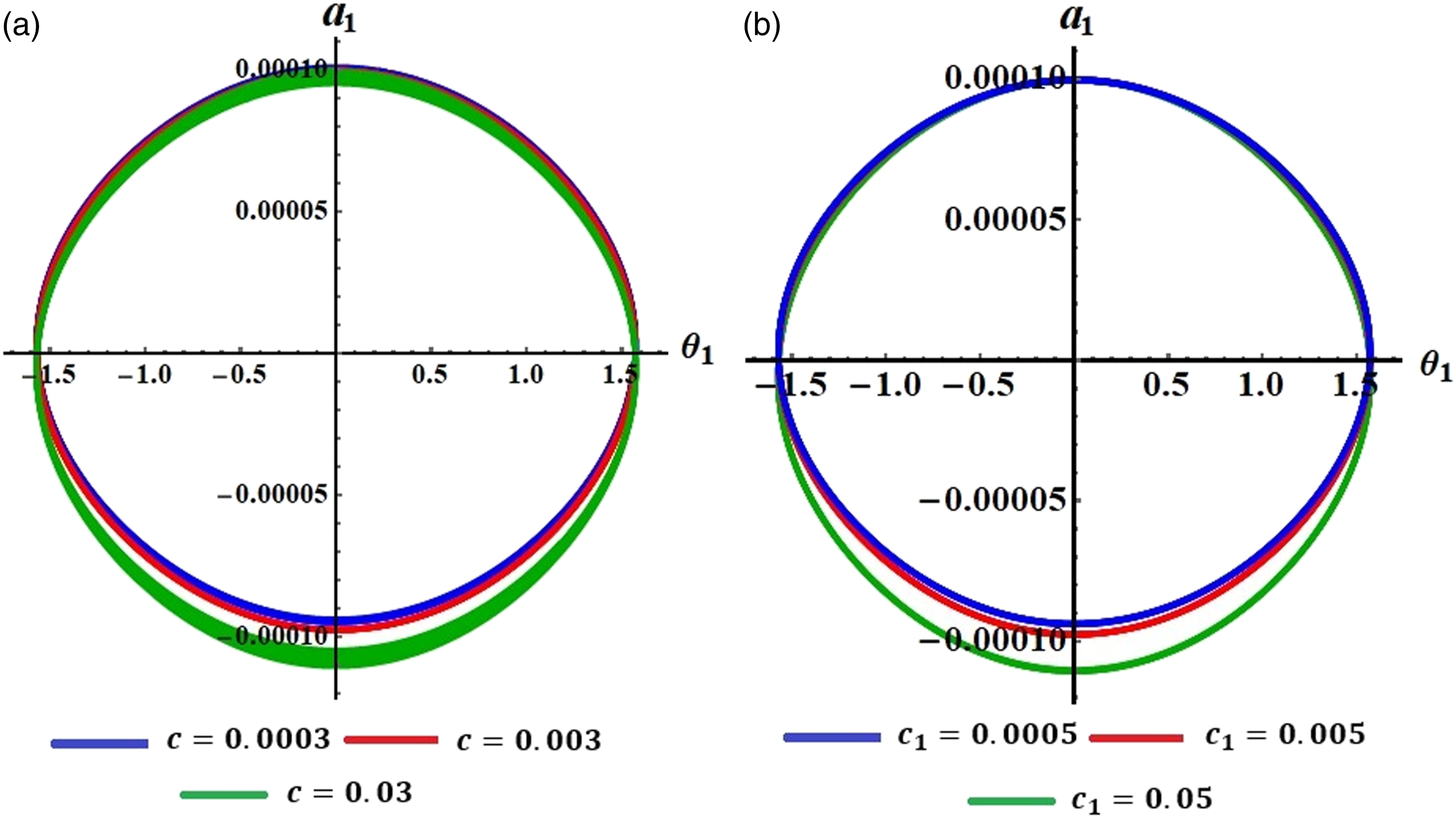
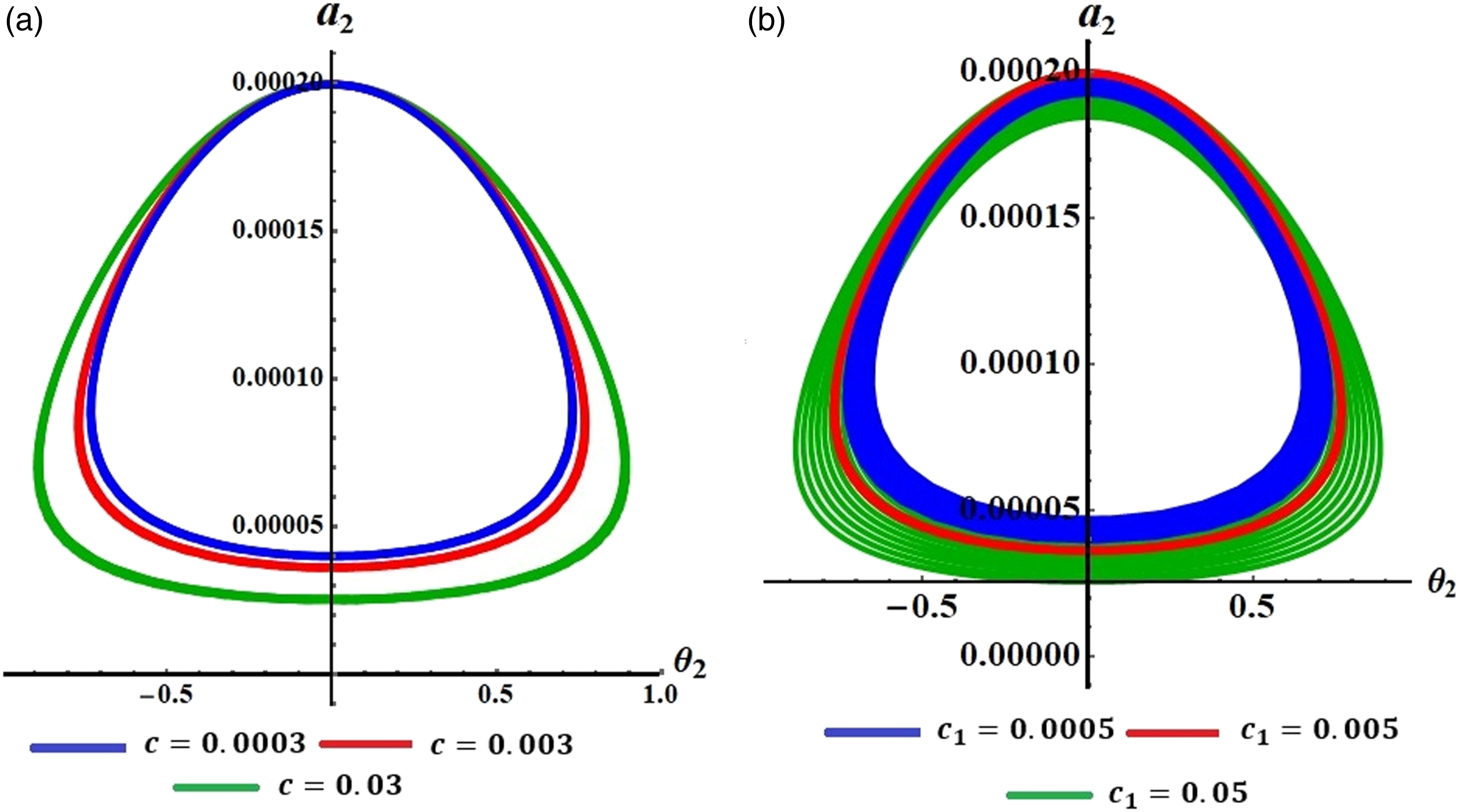
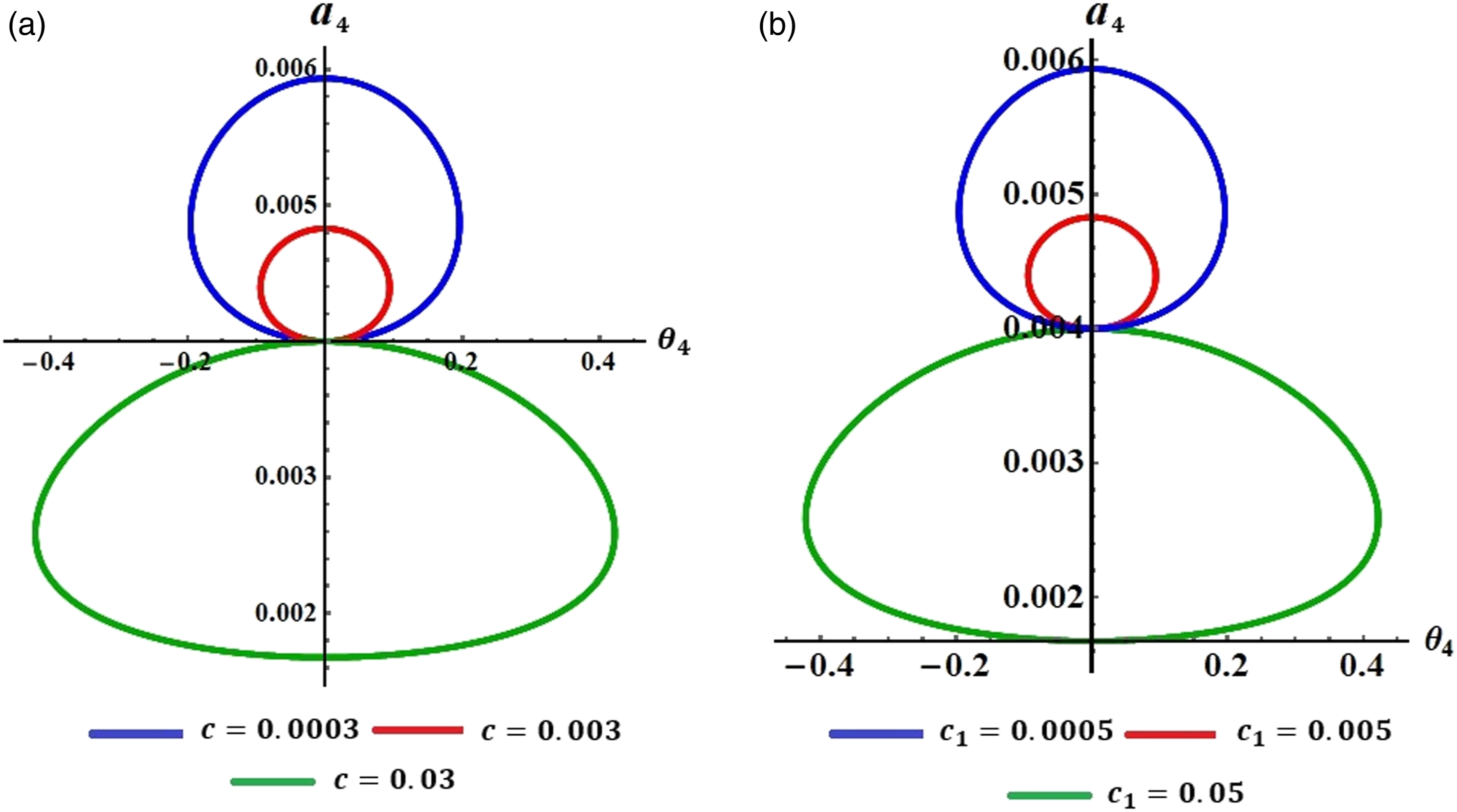
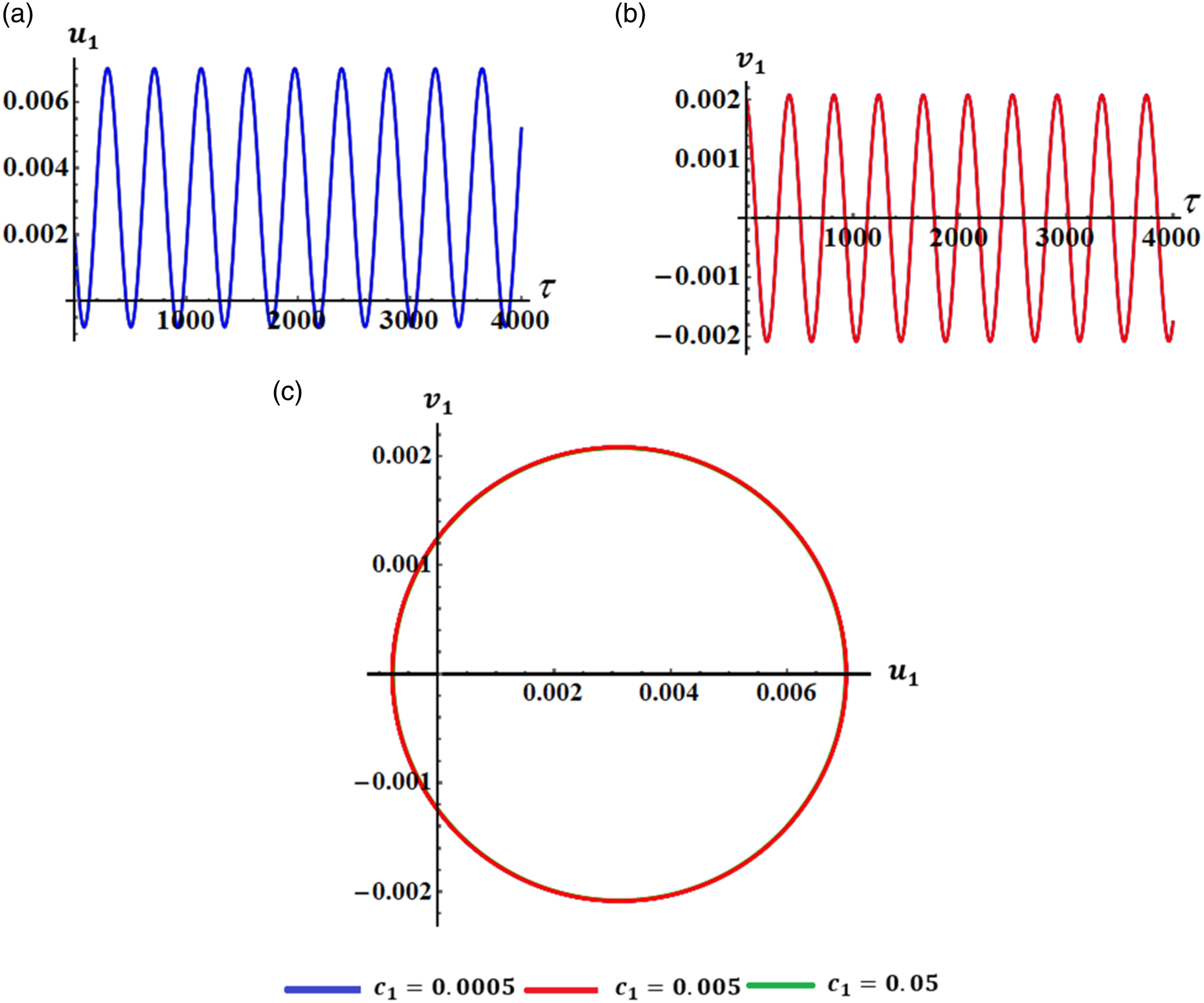
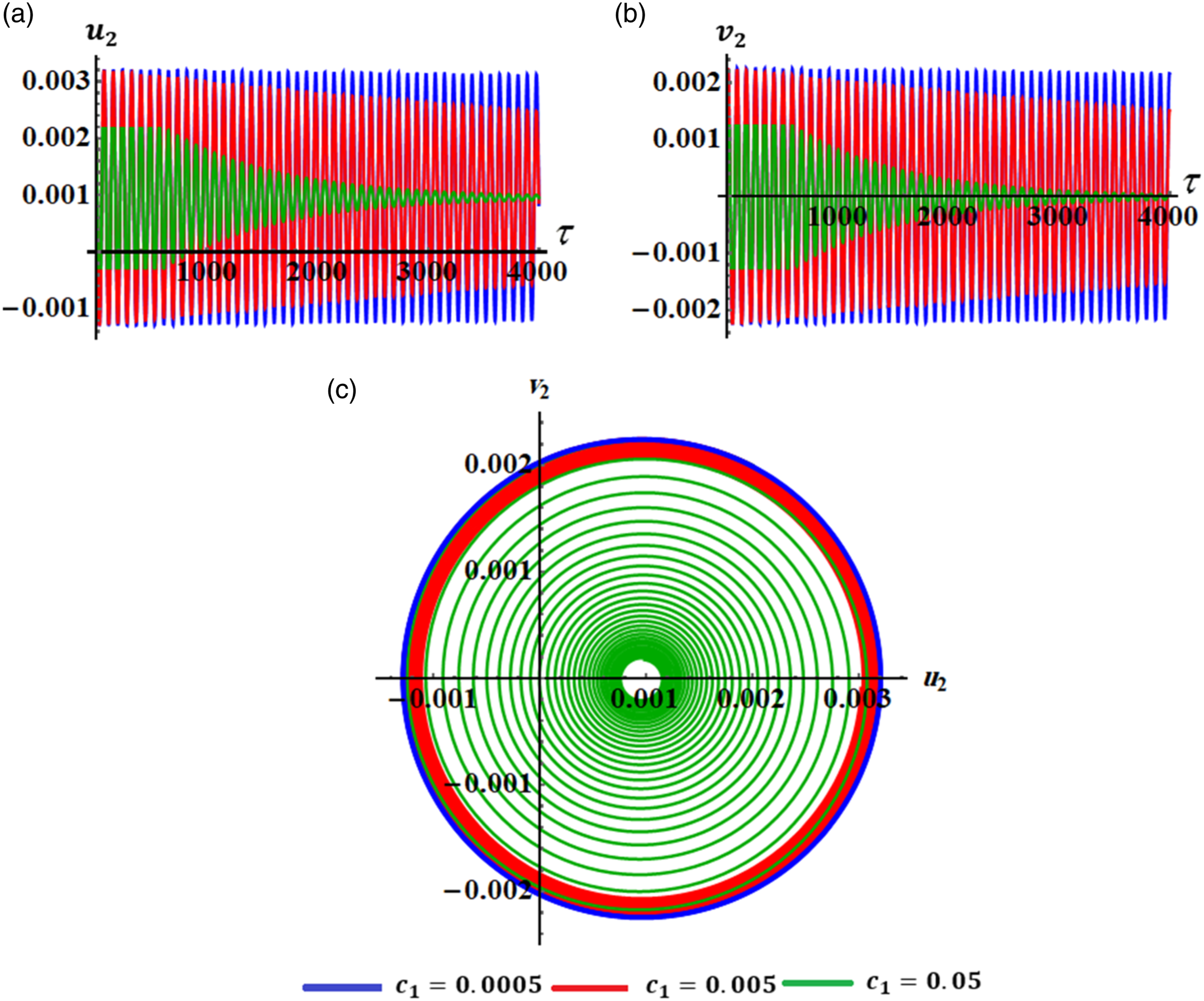
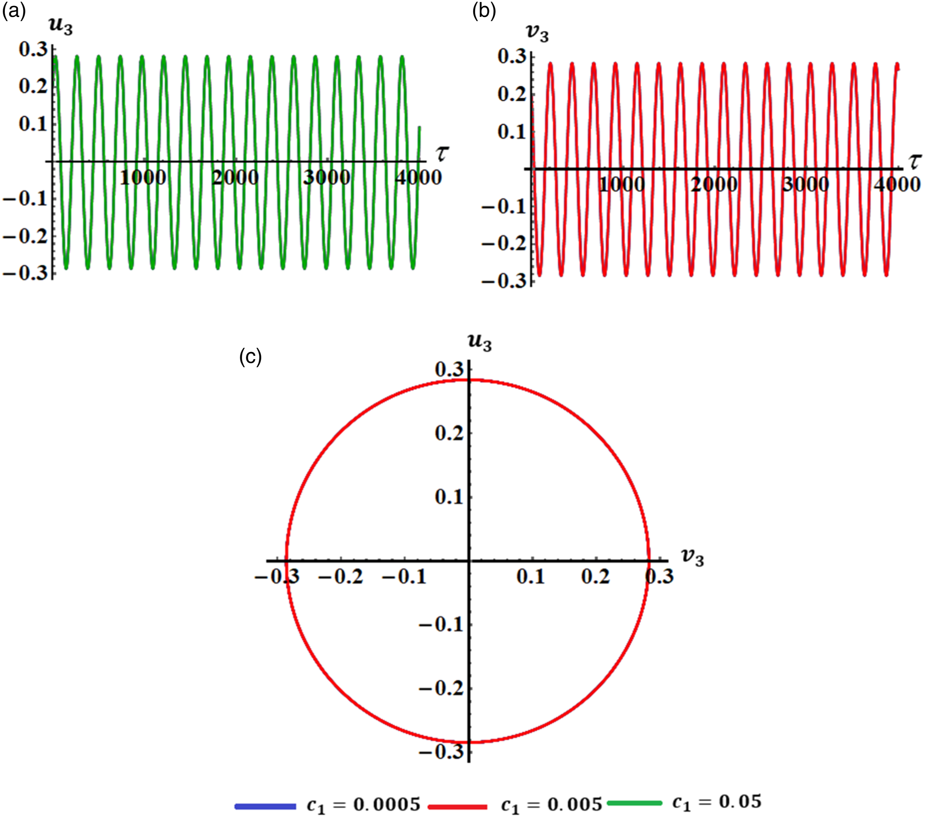
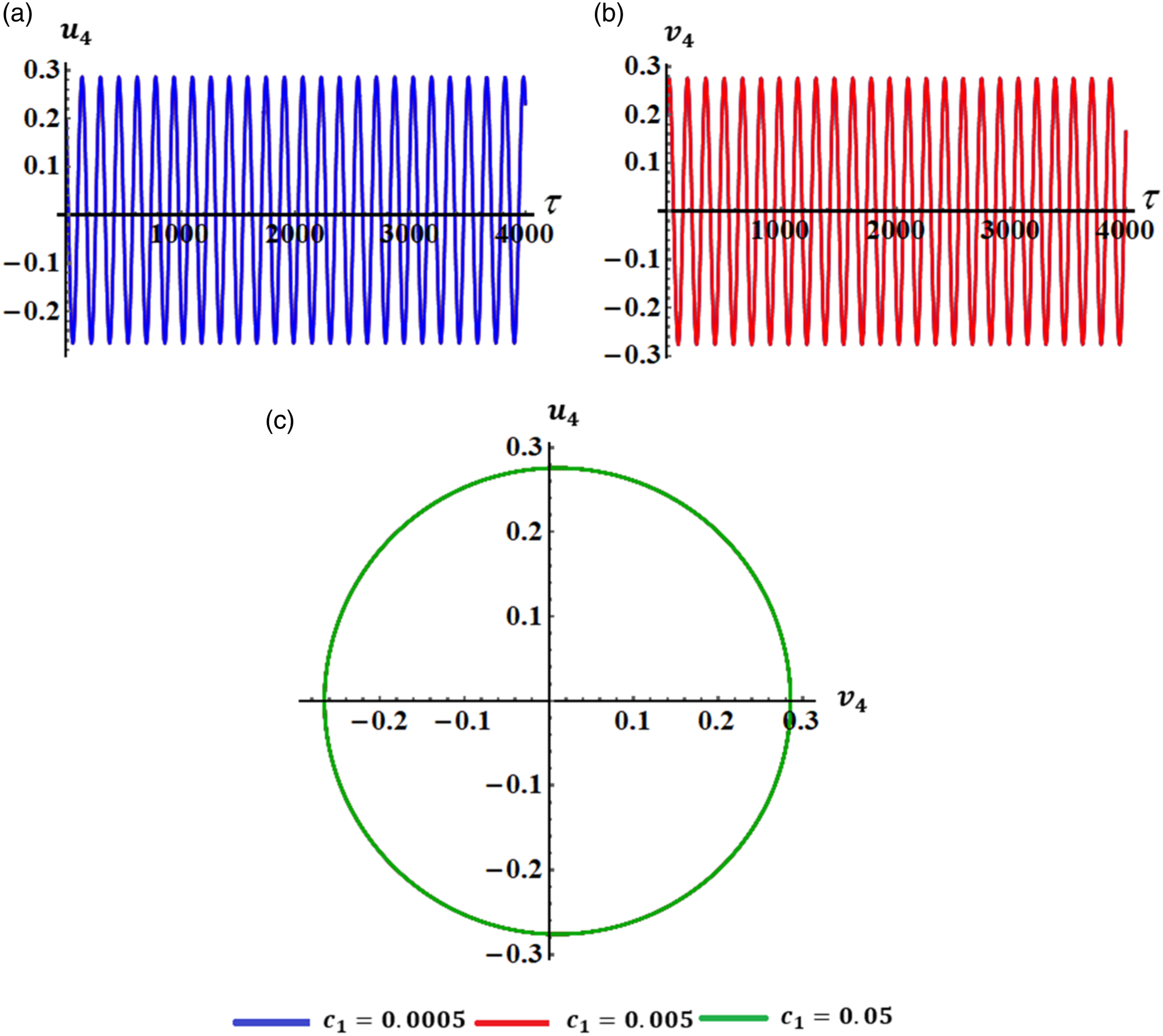
With the same above-selected data, the curves that characterize the projections of previous plotted curves in the planes are graphed in Figures 6–9. The drawn curves in Figures 6 and 7 have the form of closed curves, in which the colors that were used in Figures 2 and 3 have been adopted to indicate the corresponding behaviors. These mean that the results gained have a stable manner, as mentioned above. The periodicity of the drawn curves in parts of Figure 8 corresponds to the curves of Figure 4 when and have various values, which assert the stationary behavior of the obtained results of system (59). Moreover, the represented curves in the plane have forms of symmetric closed curves, as plotted in Figure 9, which consist with the drawn curves in Figure 5.
Describes the curves in the plane for various values of: (a) , (b) .
Shows the curves in the plane for various values of: (a) , (b) .
Explores the curves in the plane for various values of: (a) , (b) .
Represents the curves in the plane for various values of: (a) , (b) .
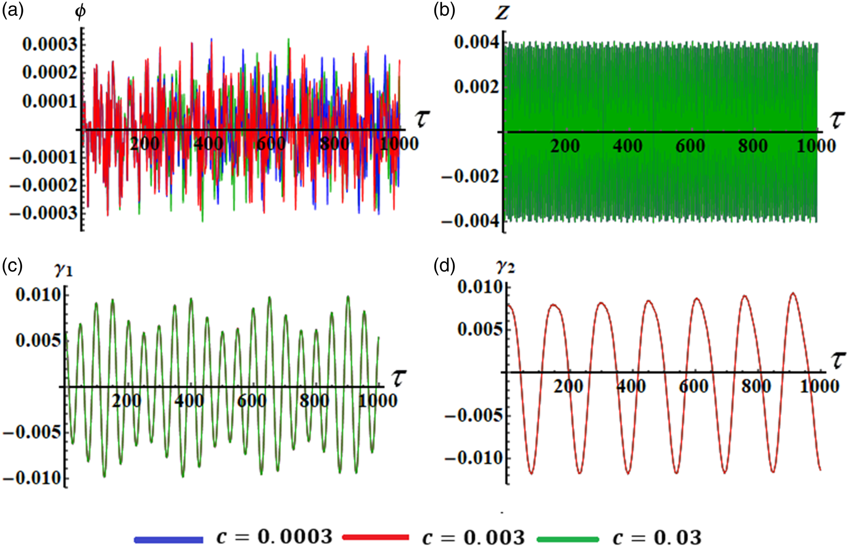
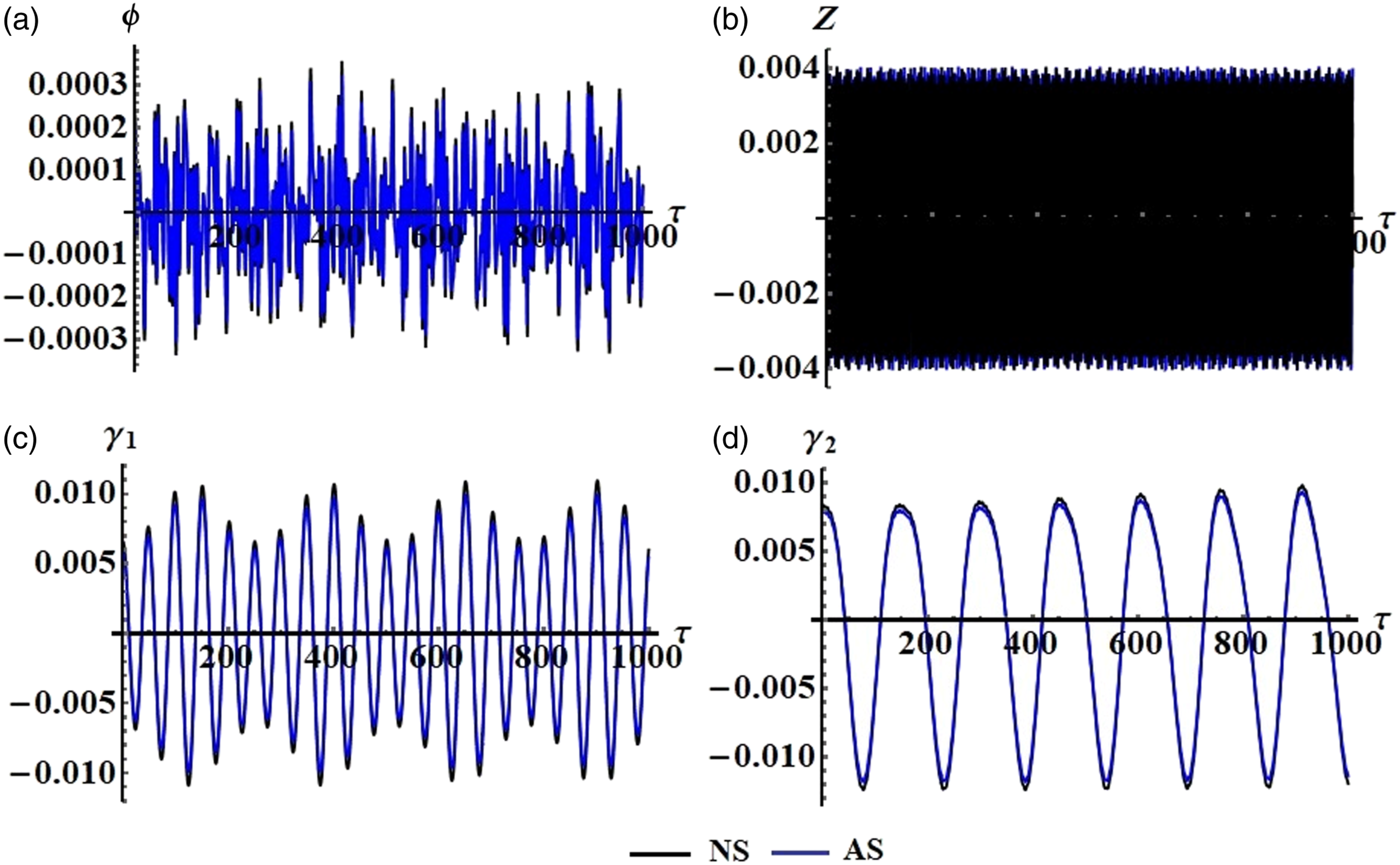
For the dimensionless time range , curves of Figure 10 shows the fluctuations of the achieved AS and when in addition to the above considered data, in which they have quasi-periodic forms. The reason of this behavior is due to the nonlinearity of the examined system. The comparison between the AS and the NS of the original governing system of motion are graphed in parts of Figure 11 at besides the aforementioned considered data of other parameters. This comparison shows good agreement between them, supporting the claim that the used perturbation approach is highly accurate.
Reveals the impact of on the solutions: (a) , (b) , (c) , and (d) .
Emphasizes the consistency between the AS and the NS when for the solutions: (a) , (b) , (c) , and (d) .
Solutions at the scenario of steady-state
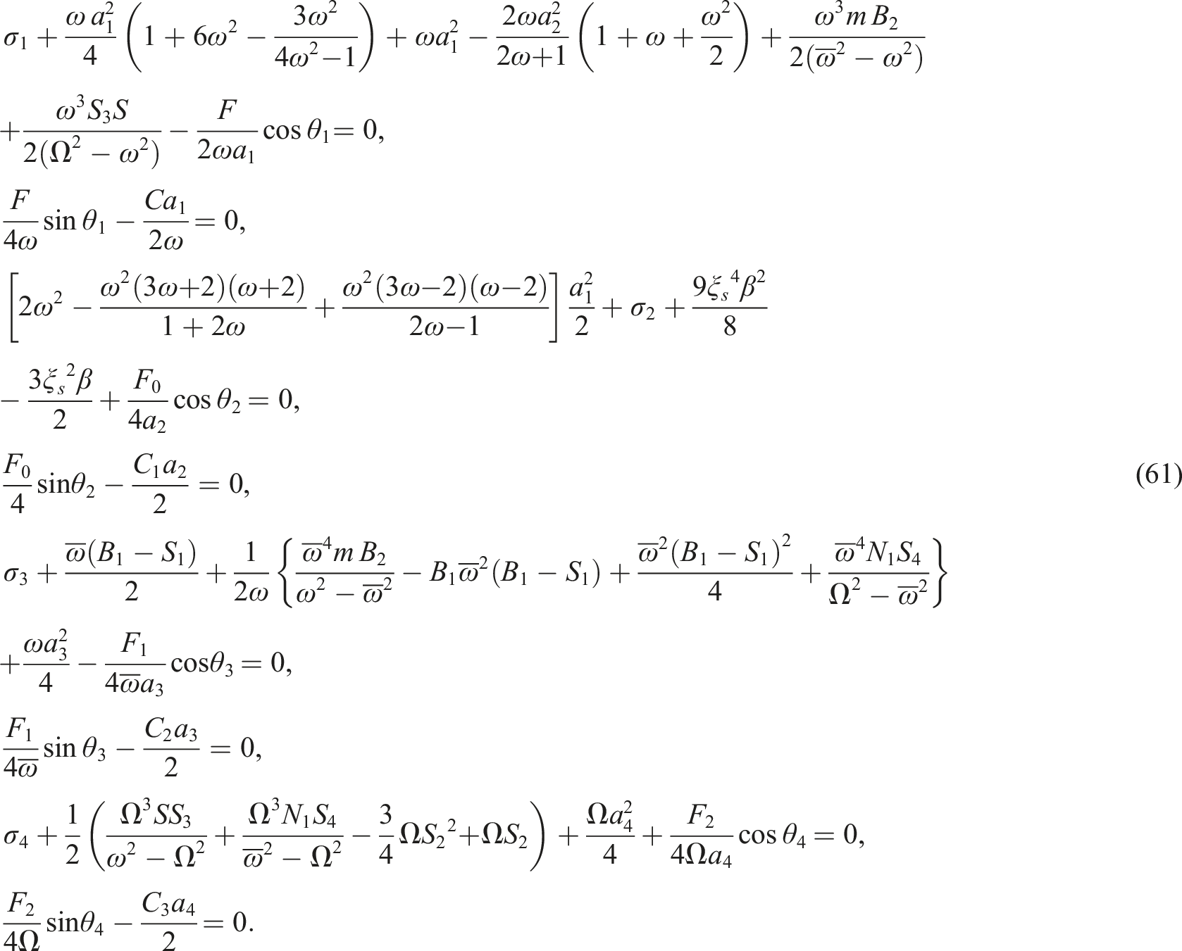
This section’s objective is to examine the vibrations of the dynamical system in a steady-state situation. In order to achieve this purpose, we take into account the zero value of and .60 Thus, a system of eight algebraic equations with respect to and is generated as follows
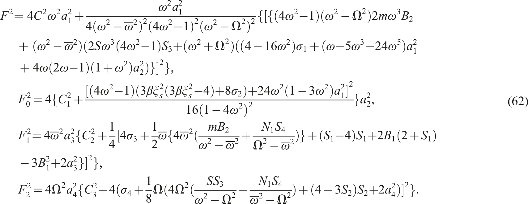
Removing from the solutions at the steady-state case, the aforementioned system’s of frequency response is produced as follows
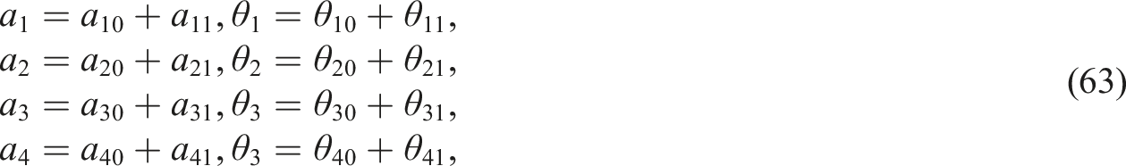
It’s crucial to keep in mind that the study of stability is regarded as a vital aspect of the research of stability. Consequently, let’s take into consideration the following replacements into the aforementioned system of equations (59) in order to investigate the behavior near a neighborhood region of fixed points61
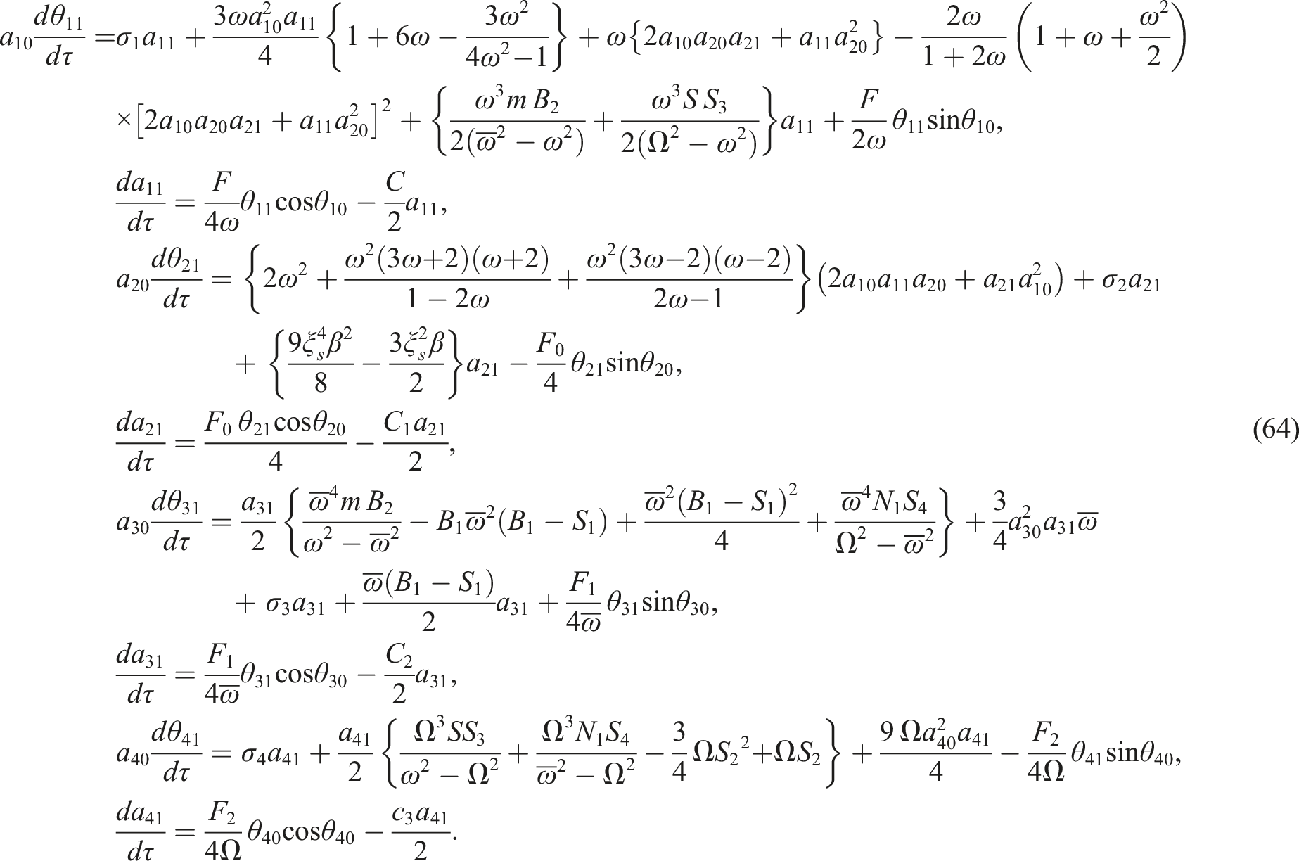
where and represent the steady-state solutions, while and are the associated perturbations, which are much smaller than and . Then, the substitution of (63) into (59) yields
If we can represent and exponentially as in the forms , where the letters and stand for constants and the eigenvalues of the unidentified perturbations associated to them. If the steady-state solutions at and are asymptotically stable, the real parts of the roots of the below characteristic equations should have negative values55
Here represent functions of and , that can be obtained easily, (see Appendix 1).
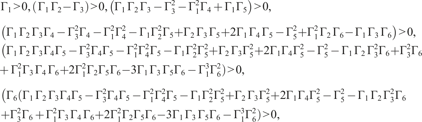
The necessary and sufficient conditions for steady-state solutions are provided by the RHC,66 which are written as follows
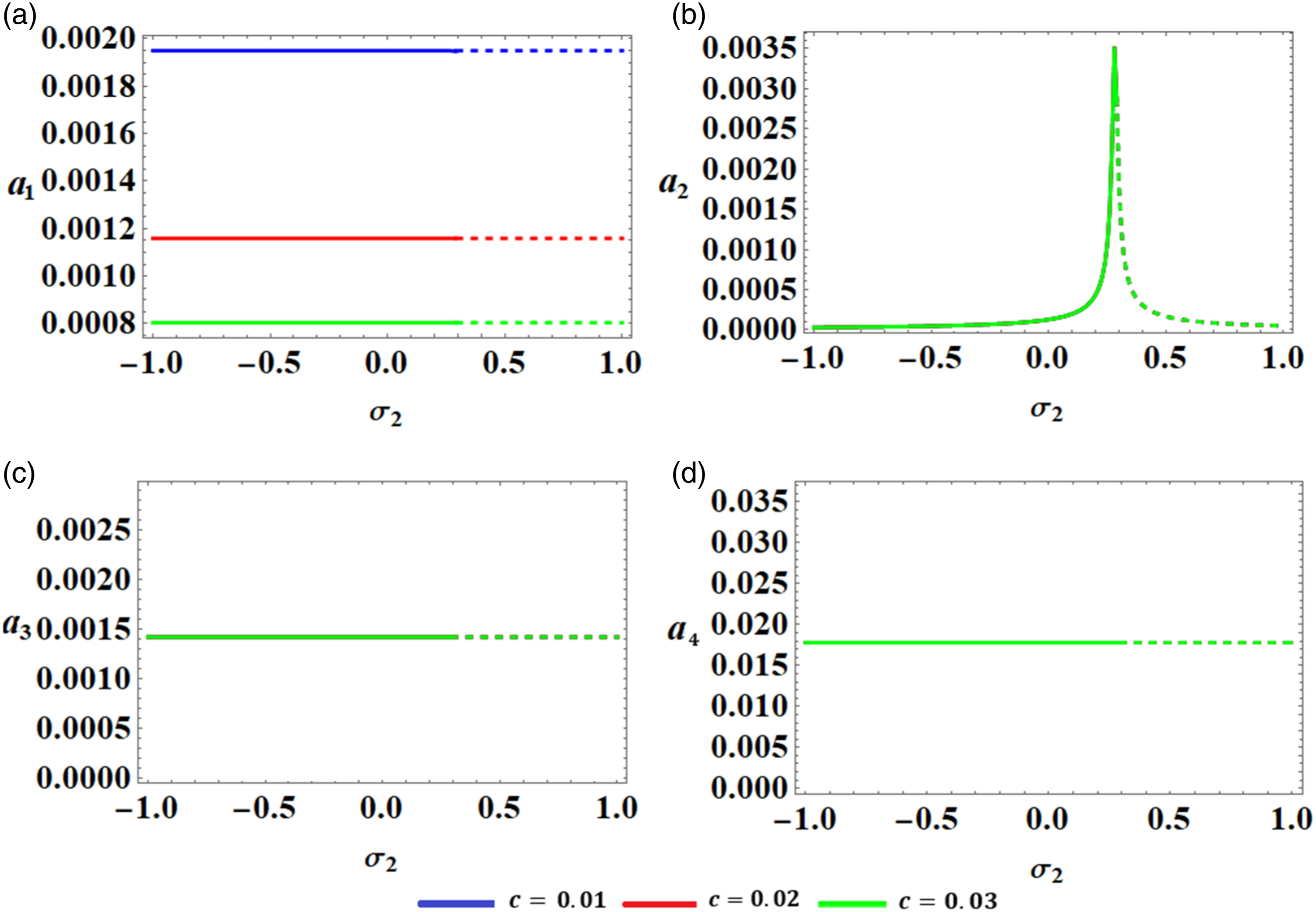
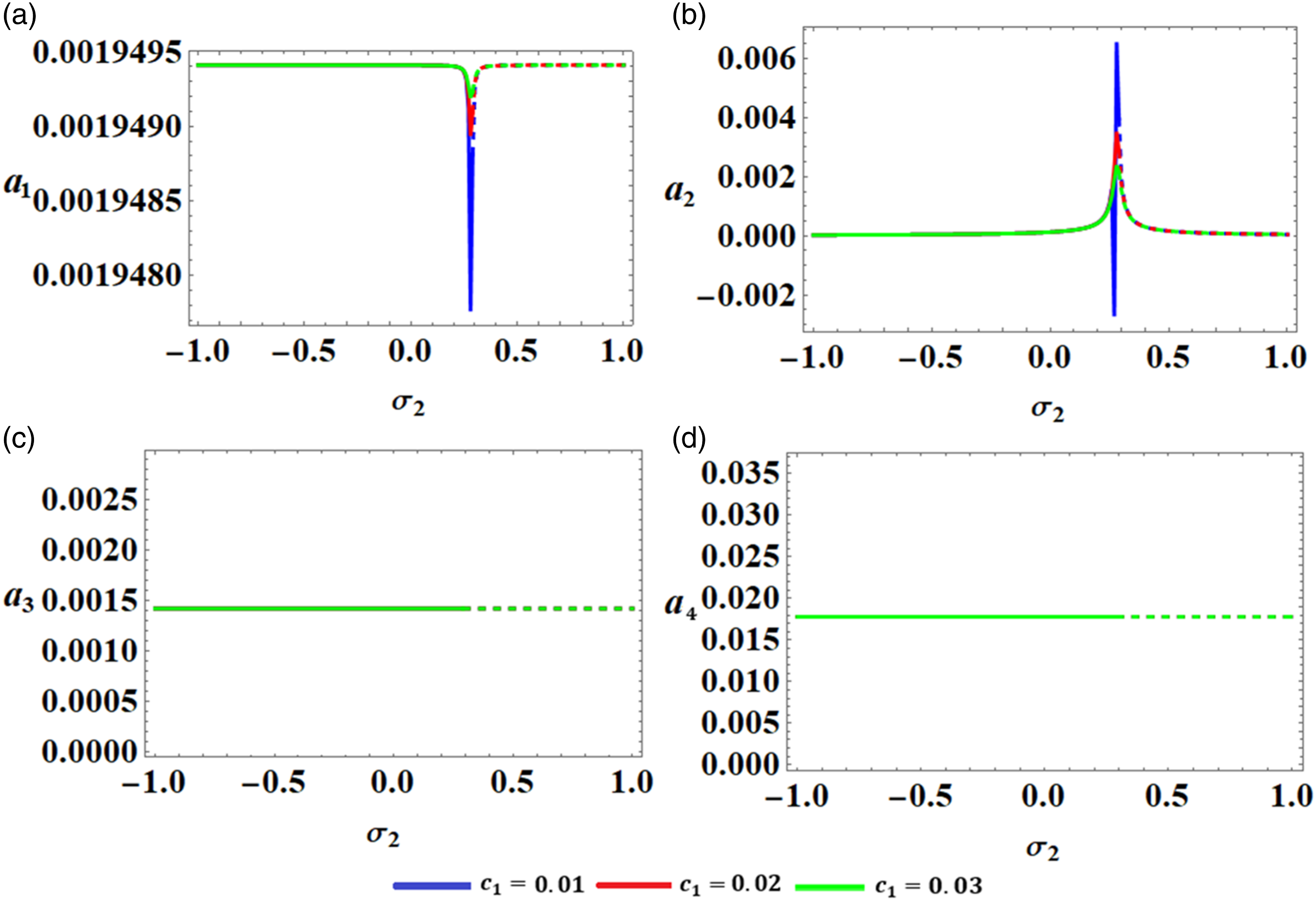
According to the above conditions (66), one can determine the stability and instability regions, in which the linear stability analysis is used to look at how the dynamical system under consideration moves under the influence of external moments. In addition to modeling of the equations of the nonlinear system, the stability criteria are carried out. It has been found that some parameters, including damping parameters and the detuning ones , are crucial in compromising the stability requirements. The system’s stability graphs have been plotted using a customized procedure of system (59) with various values of and parameters. Therefore, the frequency response curves of the amplitude and the detuning parameter as one of . Consequently, the stable and unstable areas of fixed points fall into the ranges of and , respectively, under the current limitations of the chosen values of the impacted parameters. It is significant to observe that the dashed curves represent the unstable ranges, whereas the continuous ones represent the domain of stable fixed points, as seen in Figures 12 and 13.
Displays the curves of frequency response when has various values.
Displays the curves of frequency response when has various values.
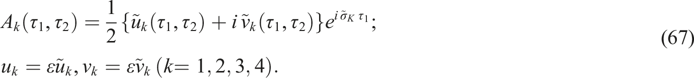
Non-linear analysis
This section demonstrates the properties of the nonlinear amplitude of equations (59) and its stability. Hence, the following relevant transformations are considered65
Here and represent the real and imaginary components of , respectively.
Substituting (19) and (67) into (55) and (56), and then separating the real portions and the imaginary ones
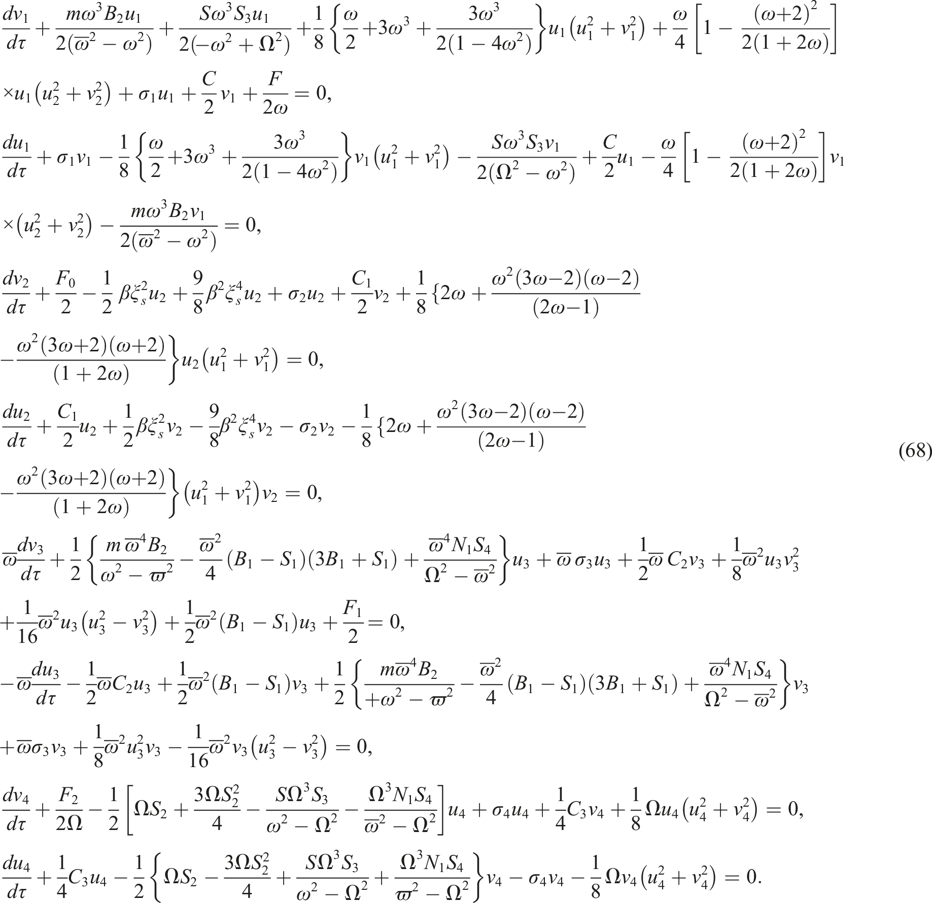
The modified amplitudes were revalidated over the entire time in different parametric domains, and the properties of the amplitude were displayed in curves of the phase plane, as shown in Figures 14–17 utilizing the below data of the parameters
Displays the behavior of: (a) , (b) , while (c) presents the trajectory’s projection of and in the plane .
Describes the behavior of: (a) , (b) , (c) the curves of phase plane
Illustrates the behavior of: (a) , (b) , while (c) presents the projections of the trajectories of (a) and (b) in the plane .
Explores the behavior of: (a) , (b) , while (c) reveals the projections of the trajectories of (a) and (b) in the plane .
A closer look at the portions of Figures 14–17 shows that their portions (a) and (b) express the variation of waves describing and with time , while the last portion (c) explores the projections of these waves in the planes . Decay waves are observed in Figures 17(a) and (b) when the damping parameter has various values through the entire period of time. Projections of these waves in the phase plane are graphed in Figure 17(c), in which their behaviors in this plane follow the forms of spiral curves directed towards one point. This means that the represented waves have stable manner during the examined interval of time.
Periodic waves of the functions and are plotted in parts (a) and (b) of Figures 15–17 with various values of . On the other side, curves of parts (c) in these figures have symmetric closed curves which assert that these waves have stable behaviors. There is no variation in the drawn curves with change of values, as seen in Figures 15 and 16, while this variation grows to some extent in the curves of Figure 17. The reason goes back to the mathematical structure of system (68).
The corresponding curves of the aforementioned ones in Figures 14–17 have been drawn in Figures 18–21. The good impact of various values of has been observed in the curves of Figure 19 for the behaviors of and the phase plane curves in , while the curves of other figures do not have any variation. The reason is due to the dependence or independency of the equations of system (68) on .
Displays the impact of on the behavior of: (a) , (b) , while (c) presents the trajectory’s projection of and in the plane .
Describes the effects of on the behavior of: (a) , (b) , (c) the curves of phase plane .
Illustrates the impact of on the behavior of: (a) , (b) , while (c) presents the projections of the trajectories of (a) and (b) in the plane .
Explores the influence of on the behavior of: (a) , (b) , while (c) reveals the projections of the trajectories of (a) and (b) in the plane .
Conclusion
The motion of a 4DOF dynamical system consisting of a connected double rigid body pendulum with a nonlinear damped spring has been examined under the effects of harmonically external moments. The GS of motion has been derived in the context of system’s generalized coordinates of through Lagrange's equations, and it has been solved analytically using MSM up to a higher order of approximation. The conditions for solvability have been attained in light of removing secular terms. Four different resonance situations are simultaneously examined after being divided into appropriate categories. The NS and AS are then compared to demonstrate their great degree of consistency and draw attention to the precision of the MSM. The influence of numerous parameters of the system has been graphically illustrated according to the graphs of motion's temporal history, steady-state solutions, and resonance curves. At steady-state conditions, all significant fixed points have been recognized and plotted through stability and instability areas, according to the RHC. The nonlinear stability analysis has been examined and discussed to assert the sable behavior of adjusted amplitudes.
Supplemental Material
Supplemental Material - Stability and analysis of the vibrating motion of a four degrees-of-freedom dynamical system near resonance
Supplemental Material for Stability and analysis of the vibrating motion of a four degrees-of-freedom dynamical system near resonance by TS Amer, AI Ismail, MO Shaker, WS Amer and HA Dahab in Journal of Low Frequency Noise, Vibration and Active Control.
Footnotes
Declaration of conflicting interests
The author(s) declared no potential conflicts of interest with respect to the research, authorship, and/or publication of this article.
Funding
The author(s) disclosed receipt of the following financial support for the research, authorship, and/or publication of this article: This study is supported by The Deanship of Scientific Research at Umm Al-Qura University for supporting this work by Grant Code: (22UQU4240002DSR18).
ORCID iDs
TS Amer
AI Ismail
WS Amer
Data availability statement
No datasets were produced or examined. Therefore, sharing of data is not appropriate for this study.
Supplemental Material
Supplemental material for this article is available online.
References
1.
StrogatzSH. Nonlinear dynamics and chaos: with applications to physics, biology, chemistry, and engineering. Boca Raton, FL: CRC Press, 2015.
2.
YuTJZhangWYangXD. Global dynamics of an autoparametric beam structure. Nonlinear Dyn2017; 88(2): 1329–1343.
3.
IkedaT. Nonlinear parametric vibrations of an elastic structure with a rectangular liquid tank. Nonlinear Dyn2003; 33(1): 43–70.
4.
CveticaninLZukovicMCveticaninD. Oscillator with variable mass excited with non-ideal source. Nonlinear Dyn2018; 92: 673–682.
5.
NayfehAH. Introduction to perturbation techniques. Hoboken, NY: John Wiley & Sons, 2011.
6.
HolmesMH. Introduction to perturbation methods. Berlin: Springer Science & Business Media, 2012.
Al-LehaibiE. The vibration of a viscothermoelastic gold nanobeam induced by different types of thermal loading. Journal of Umm Al-Qura University for Applied Science2020; 6: 6–13.
9.
YoussefHMAl ThobaitiAA. The vibration of a thermoelastic nanobeam due to thermo-electrical effect of graphene nano-strip under Green-Naghdi type-II model. Journal of Engineering and Thermal Sciences2022; 2(1): 1–12.
10.
Al-LehaibiE. The vibration of a gold nanobeam under the thermoelasticity fractional-order strain theory based on Caputo-Fabrizio’s definition. J Strain Analysis2023; 58: 464. DOI: 10.1177/03093247221145792.
11.
ChirikovBV. Resonance processes in magnetic traps. J. Nucl. Energy C Plasma Phys1960; 1: 253–260.
12.
ChirikovBV. A universal instability of many-dimensional oscillator systems. Phys Rep1979; 52: 263–379.
13.
LichtenbergAJLiebermanMA. Regular and chaotic dynamics. New York, NY: Springer, 1992.
14.
EissaMSayedM, A comparison between active and passive vibration control of non-linear simple pendulum, part I: transversally tuned absorber and negative feedback, Math Comput Appl2006; 11(2): 137–149.
15.
EissaMSayedM, A comparison between active and passive vibration control of non-linear simple pendulum, part II: longitudinal tuned absorber and negative and feedback, Math Comput Appl2006; 11(2): 151-162.
16.
EissaM. Vibration reduction of a three DOF non-linear spring pendulum. Commun Nonlinear Sci Numer Simul2008; 13: 465–488.
17.
LeeWKHsuCS. A global analysis of an harmonically excited spring-pendulum system with internal resonance. J Sound Vib1994; 171(3): 335–359.
GilatA. Numerical methods for engineers and scientists. New York, NY: Wiley, 2013.
20.
AgrawalAKYangJNWuJC. Non-linear control strategies for duffing systems. Int J Non Lin Mech1998; 33(5): 829–841.
21.
AmerTSBekMA. Chaotic responses of a harmonically excited spring pendulum moving in circular path. Nonlinear Anal. RWA2009; 10(5): 3196–3202.
22.
BelyakovAO. On rotational solutions for elliptically excited pendulum. Phys Lett2011; 375: 2524–2530.
23.
IsmailAI. Relative periodic motion of a rigid body pendulum on an ellipse. J Aero Eng2009; 22(1): 67–77.
24.
AmerTS. The dynamical behavior of a rigid body relative equilibrium position. Adv Math Phys2017; 2017: 13.
25.
StarostaRKaminskaGAwrejcewiczJ. Asymptotic analysis of kinematically excited dynamical systems near resonances. Nonlinear Dyn2012; 68: 459–469.
26.
AmerTSBekMAHamadaIS. On the motion of harmonically excited spring pendulum in elliptic path near resonances. Adv Math Phys2016; 2016: 15.
27.
StarostaRKamińskaGAwrejcewiczJ. Parametric and external resonances in kinematically and externally excited nonlinear spring pendulum. Int J Bifurc Chaos2011; 21: 3013–3021.
28.
AwrejcewiczJStarostaRKamińskaG. Asymptotic analysis and limiting phase trajectories in the dynamics of spring pendulum. Applied non-linear dynamical systems, springer proceedings in mathematics and statistics. New York, NY: Springer, 2014, Vol. 93, pp. 161–173.
29.
AwrejcewiczJStarostaRKamińskaG. Asymptotic analysis of resonances in nonlinear vibrations of the 3-DOF pendulum. Differ. Equ. Dyn. Syst2013; 21: 123–140.
FossenTINijmeijerH. Parametric resonance in dynamical systems. Berlin: Springer Science + Business Media, LLC, 2012.
37.
ZhuSJZhengYFFuYM. Analysis of non-linear dynamics of a two-degree-of-freedom vibration system with non-linear damping and non-linear spring. J Sound Vib2004; 271: 15–24.
38.
El RifaiKHallerGBajajAK. Global dynamics of an autoparametric spring-mass-pendulum system. Nonlinear Dyn2007; 49: 105–116.
39.
KęcikKWarminskiJ. Dynamics of an autoparametric pendulum-like system with a nonlinear semiactive suspension. Math Probl Eng2011; 2011: 15. Article ID 451047.
40.
KęcikKMituraAWarmińskiJ. Efficiency analysis of an autoparametric pendulum vibration absorber. Eksploat. Niezawodn2013; 15(3): 221–224.
41.
Vazquez-GonzalezBSilva-NavarroG. Evaluation of the autoparametric pendulum vibration absorber for a Duffing system. Shock Vib2008; 15: 355–368.
42.
KhirallahK. Autoparametric amplification of two nonlinear coupled mass-spring systems. Nonlinear Dyn2018; 92: 463–477.
43.
NabergojRTondlAViragZ. Autoparametric resonance in an externally excited system. Chaos, Solit Fractals1994; 4(2): 263–273.
44.
KamelM. Bifurcation analysis of a nonlinear coupled pitch-roll ship. Math Comput Simulat2007; 73(5): 300–308.
45.
ZhouLChenF. Stability and bifurcation analysis for a model of a nonlinear coupled pitch-roll ship. Math Comput Simulat2008; 79(2): 149–166.
46.
AnjumNHeJ-H. Two modifications of the homotopy perturbation method for nonlinear oscillators. J. Appl. Comput. Mech2020; 6(SI): 1420–1425.
47.
AnjumNHeJ-H. Higher-order homotopy perturbation method for conservative nonlinear oscillators generally and microelectromechanical systems’ oscillators particularly. Int J Mod Phys B2020; 34(32): 2050313. (Pages 9).
48.
AnjumNHeJ. Homotopy perturbation method for N/MEMS oscillators. Math Methods Appl Sci2020: 1–15. DOI: 10.1002/mma.6583.
49.
AnjumNHeJ-HAinQT, et al.Li-He’s modified homotopy perturbation method for doubly-clamped electrically actuated microbeams-based micreoelectromechanical system. Facta Univ–Ser Mech Eng2021; 19(4): 601–612.
50.
HeC-HTianDMoatimidGM, et al.Hybrid Rayleigh–van der pol–doffing oscillator: stability analysis and controller. J Low Freq Noise Vib Act Control2022; 41(1): 244–268.
51.
HeJHYangQHeCH, et al.Pull-down instability of the quadratic nonlinear oscillators. Facta Univ Ser: Mech Eng2023; 21: 191. DOI: 10.22190/FUME230114007H.
52.
FengGQNiuJY. The analysis for the dynamic pull-in of a micro-electromechanical system. J Low Freq Noise Vib Act Control2023; 42(2): 558–562.
53.
NiuJY. Pull-down plateau of a Toda-like fractal-fractional oscillator and its application in grass carp’s roes’ agglomeration. J Low Freq Noise Vib Act Control2023; 42: 1775. DOI: 10.1177/14613484231185490.
54.
AmerTSMoatimidGMAmerWS. Dynamical stability of a 3-DOF auto-parametric vibrating system. J. Vib. Eng. Technol2022; 11: 4151. DOI: 10.1007/s42417-022-00808-1.
55.
AmerTSIsmailAIAmerWS. Evaluation of the stability of a two degrees-of-freedom dynamical system. J Low Freq Noise Vib Act Control2023; 42: 1578. DOI: 10.1177/14613484231177654.
56.
WojnaMWijataAWasilewskiG, et al.Numerical and experimental study of a double physical pendulum with magnetic interaction. J Sound Vib2018; 430: 214–230.
57.
PolczyńskiKWijataAAwrejcewiczJ, et al.Numerical and experimental study of dynamics of two pendulums under a magnetic field. Proc IMechE Part I: J Systems and Control Engineering2019; 233(4): 441–453.
58.
AmerTSBekMAAbouhmrMK. On the motion of a harmonically excited damped spring pendulum in an elliptic path. Mech Res Commun2019; 95: 23–34.
59.
El-SabaaFMAmerTSGadHM, et al.On the motion of a damped rigid body near resonances under the influence of harmonically external force and moments. Results Phys2020; 19: 103352.
60.
AbadyIMAmerTSGadHM, et al.The asymptotic analysis and stability of 3DOF non-linear damped rigid body pendulum near resonance. Ain Shams Eng J2022; 13: 101554.
61.
AbdelhfeezSAAmerTSElbazRF, et al.Studying the influence of external torques on the dynamical motion and the stability of a 3DOF dynamic system. Alex Eng J2022; 61: 6695–6724.
62.
HeC-HAmerTSTianD, et al.Controlling the kinematics of a spring-pendulum system using an energy harvesting device. J Low Freq Noise Vib Act Control2022; 41(3): 1234–1257.
63.
HeJ-HAmerTSEl-KaflyHF, et al.Modelling of the rotational motion of 6-DOF rigid body according to the Bobylev-Steklov conditions. Results Phys2022; 35: 105391.
64.
AmerAAmerTSEl-KaflyHF. Dynamical analysis for the motion of a 2DOF spring pendulum on a Lissajous curve. Sci Rep2023; 13: 21430.
65.
HeJ-HMoatimidGMZekryMH, Forced nonlinear oscillator in a fractal space, Facta Univ – Ser Mech Eng2022; 20(1): 1–20.
66.
StrogatzSH. Nonlinear dynamics and chaos: with applications to physics, biology, chemistry, and engineering. 2nd ed.Princeton, NJ: Princeton University Press, 2015.
Supplementary Material
Please find the following supplemental material available below.
For Open Access articles published under a Creative Commons License, all supplemental material carries the same license as the article it is associated with.
For non-Open Access articles published, all supplemental material carries a non-exclusive license, and permission requests for re-use of supplemental material or any part of supplemental material shall be sent directly to the copyright owner as specified in the copyright notice associated with the article.