Sufficiently small rotations of Lagrange’s gyro

Abstract

In this study, the motion of Lagrange’s gyro about its fixed point in the presence of a perturbed torque, a gyroscopic torque, and a varied restoring one is searched. We assume sufficiently small angular velocity components in the direction of the principal axes that differ from the dynamical symmetry one and a restoring torque that is considered to be greater than the perturbing one. In this manner, we replace the familiar small parameter that was used in previous works with a large one. In such cases, the gyro equations for motion (EOM) are formulated in the form of a two-degrees-of-freedom (DOF) autonomous system. We average the obtained system to get periodic solutions and motion’s geometric interpretation of the problem using the large parameter. The regular precession and the pure rotation of the motion are obtained. A numerical study is evaluated for asserted the used techniques and showed the influence of the changing parameters of motion on the gyro behavior. The trajectories of the motions and their stabilities are discussed and analyzed. The novelty of this work lies in how to adapt the method of large parameter (MLP) to solve the rigid body problem, especially since it has been assumed initially that its angular velocity or its initial energy are very small.

MSC (2000): 70E20, 70E17, 70E15, 70E05

Introduction

The problems of rotational motion of solid bodies around a fixed point in space are among the most important problems in classical mechanics. The importance of this issue is due to the significant and vital applications on large scales in mechanics, whether in civilian or military life, as well as in our daily lives. For example, but not limited to, gyroscopic movements are considered an essential application of these issues. These gyroscopes are used in aircraft, submarines, spaceships, missiles, and a very large number of different vehicles, military and civil industries, such as radars, and in other user devices in our daily lives.^1–4

Perturbation methods^5–7 have been used recently, on a large scale, to find the approximate solutions (AS) of the spatial motion of the rigid body (RB), as it is difficult to obtain the general solutions to this problem because they necessarily need a fourth initial integration according to Jacobi’s theory. The general form of this integral was not yet obtained, but it was found in famous special cases that impose restrictions on the coordinates of the center of gravity and the values of the principal moments of inertia of the RB.^8,9 Among these methods are the modifications of the small parameter method (MSPM), the averaging approach (AA), the Krylov–Bogoliubov–Mitropolski technique (KBMT), the multiple-scales approach (MSA), the method of the MLP, and others.

When the movement of RB is taken into account while being impacted by a gravitational field, a Newtonian field (NF), an electromagnetic field (EMF), and the existence of a gyro torque (GT), the MSPM is employed in^10–22 to find its AS in^10,11 under the action of a uniform gravity field, while ¹² looks into how the NF affects on the RB motion. It should be mentioned that when the frequency of the system had integer values or their multiple inverses, the resulting solutions consisted of discrete singular points. When the motion is impacted by the third component of the GT besides the NF, all singularities have been permanently resolved. ¹³ The criteria of the Kovalevskaya and Euler–Poinsot cases, respectively, were applied to the RB movement in ¹⁴ and ¹⁵ when the impact of all components of GM was taken into consideration. It was found that for any value of the system’s frequency, the resulting solutions were entirely devoid of any singularities. This method was recently used in ¹⁶ to explore how the RB moved in compliance with Bobylev–Steklov criteria while the body was being impacted by the EMF, the GT, and the NF. When the EMF and the GT were acted on the body, the authors of ¹⁷ hypothesized that the center of mass is shifted somewhat from the body axis of dynamical symmetry. The acquired results are regarded as a generalization of those found in ¹⁸ and. ¹⁹ See ^20–22 for further details on how the strategy of this method might be used to address different SB issues.

The KBMT is used in^2,23–25 to obtain the AS of the RB under the influence of a gravitational field. ²³ The gained results were generalized in ² and, ²⁴ respectively, when the body was subject to NF and GT. The authors of ²⁵ constrained the body’s motion so that its inertia ellipsoid was almost equal to its inertia rotation. It ought to be noted that, in contrast to the equivalent solutions in,^2,24,25 the solutions that have been created in ²³ include singular points when the body’s frequency comprises integer data or their inverses. This is because a new frequency, which depends on the GT, was employed in.^23–24

Over the past 40 years, the AA has been employed frequently to find the AS for a symmetric RB’s spinning motion.^26–31 This motion has been studied in three different cases: when the body was impacted by a uniform gravity field,^26,27 an NF,^28,29 and the action of a GT.^22,23 The effect of perturbing moments on a body’s motion has been taken into account. The guiding EOM is constructed using the basic equation of the RB angular momentum, where a tiny parameter was added by using some applied assumptions. Therefore, the AS of the averaging systems of the EOM is obtained. According to, ³⁰ in addition to the effects of the EMF on the RB, its inertia ellipsoid and rotations are also thought to be closely related. The generalization of this work is found in. ³¹

The motivation of this study resides in the adaptation of the MLP to the rigid body problem, especially given the initial assumption that the rigid body’s angular velocity or initial energy are relatively minimal. When perturbing, gyroscopic, and restoring torques are present, Lagrange’s gyro’s motion around its fixed point is investigated. Two assumptions are assumed; restoring torque, which is assumed to be higher than the perturbing torque, and sufficiently tiny angular velocity components in the direction of the primary axes that diverge from the dynamical symmetry one. In this way, we swap out the familiar tiny parameter that was utilized in earlier studies for a large one. In these circumstances, the gyro EOM is expressed as a 2DOF autonomous system. Utilizing the MLP, we average this system to obtain the desired periodic solutions. The possible regular precession and pure rotation of the body’s motion are acquired. The effectiveness of the employed methods is assessed using a numerical analysis, ³² which also demonstrated the impact of varying parameters on the behavior of the gyro’s motion. The motion and stability trajectories are discussed and analyzed in a suitable manner.^33,34 There are no restrictions on the body’s motion about the third principal axis, as in previous works, and the body will be given small energies initially for the motion instead of high energies as in previous works.

Description of the problem

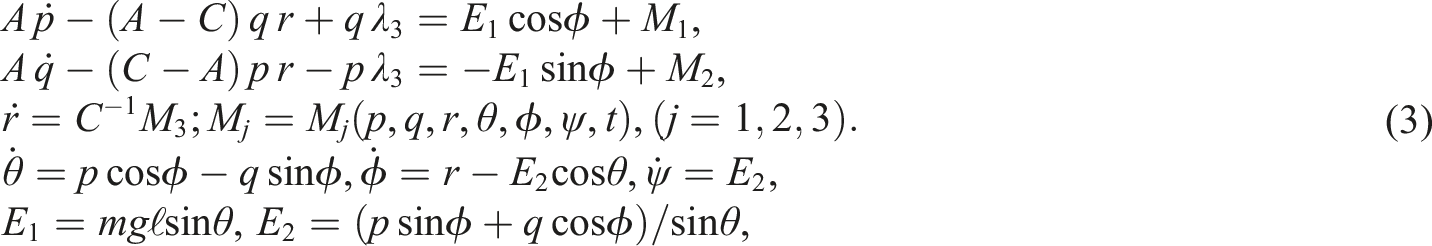
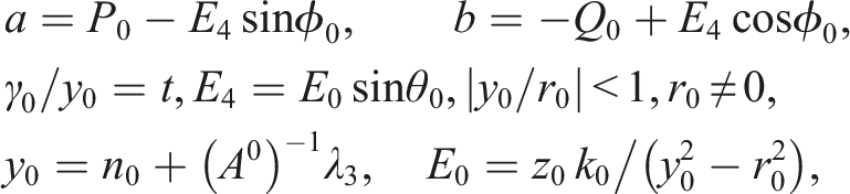
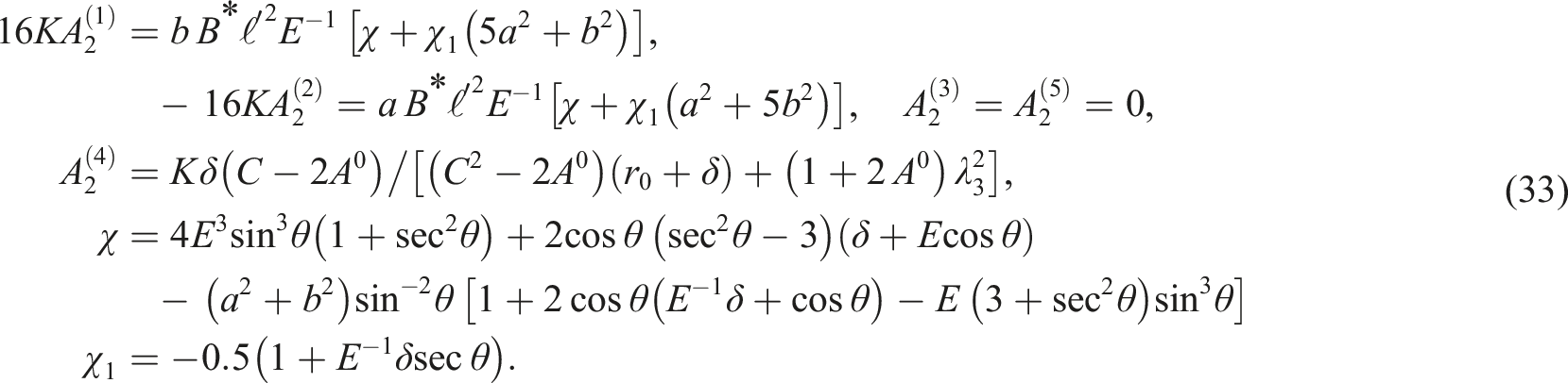
As an extension of this field of study, we present a problem’s description of a rotatory motion of a gyro with a mass $m$ about a fixed origin point $O$ of two frames; $OXYZ$ is a fixed frame in space where $OZ$ is considered to be a downward direction and a mobile frame $Oxyz$ whose axes are directed along the body’s principal axes of inertia. The action of a gyrostatic torque ${\lambda }_3$ about the moving $Oz$ -axis and a restoring torque , comes from a unit charge on the $Oz$ -axis, a magnetic field of strength ${\underset{¯}{B}}^{*}$ , and a perturbing torque $\underset{¯}{M}\equiv (M_1,M_2,M_3)$ is considered. It is assumed that the gyro has sufficiently small angular velocities about $Ox$ and $Oy$ axes, in addition to the restoring torque is large compared with the perturbed vector torque acting on the principal inertia gyro’s axes. Therefore, a large parameter $\epsilon \gg 1$ ^35,36,37 can be inserted in the EOM and therefore, the AA^6,7,38 can be used to average the gyro’s system of motion, which can be to determine Euler’s angles. The geometric illustrations are given as a function of $t$ and the body’s parameters. Consider the gyro-rotation ellipsoid that coincides with its ellipsoid of inertia, and the body’s center of mass $\left(x_c,y_c,z_c\right)$ is displaced by a distance of the order ${\epsilon }^{-1}$ .Then, the principal inertia moments $\left(A,B,C\right)$ and $\left(x_c,y_c,z_c\right)$ become^31,39

$A\epsilon =A^0\left(\epsilon +{\delta }_1\right),B\epsilon =A^0\left(\epsilon +{\delta }_2\right),A^0\ne C$

(1)

$x_c\epsilon =x_1 \ell ,y_c\epsilon =y_1 \ell ,z_c=\ell ,$

(2)

where ${\delta }_i\hspace{0.17em}\left(i=\mathrm{1,2}\right)$ are dimensionless constants of order unity, the symbol $A^0$ mentioned above is the characteristic value for inertia moments; $\left(x_1,y_1\right)$ are dimensionless finite quantities compared with $1/\epsilon$ , and $\ell$ represents a distance from the center of mass to $O$ .

We will extract the moment caused by the electromagnetic field to learn more about the gyrostatic motion. Consequently, the Lorentz force $-({\underset{¯}{B}}^{*}\wedge \underset{¯}{V})$ ⁴⁰ is utilized such that $\underset{¯}{V}=-(\underset{¯}{{\ell }^{\prime }}\wedge \underset{¯}{\omega })$ and $\underset{\_}{{\ell }^{\prime }}\equiv \left(\mathrm{0,0},{\ell }^{\prime }\right)$ where $\underset{\_}{{\ell }^{\prime }}$ is the position vector between the unit charge and $O$ , and $\underset{¯}{\omega }\equiv (p,q,r)$ is the gyro’s angular velocity. Then, the targeted moment has the form $\underset{¯}{M}=-(\underset{¯}{{\ell }^{\prime }}.{\underset{¯}{B}}^{*})(\underset{¯}{{\ell }^{\prime }}\wedge \underset{¯}{\omega })$ with the following three components $B^{*}{\ell }^{\prime 2}\cos \theta \left(q,-p,0\right)$ in the direction of the gyro principal axes of inertia, where $\theta$ is the angle of nutation.

Therefore, Euler’s dynamic EOM becomes^29,31

$\begin{array}{l}A \dot{p}-\left(A-C\right) q r+q {\lambda }_3=E_1 \cos \varphi +M_1,\\ A \dot{q}-\left(C-A\right) p r-p {\lambda }_3=-E_1 \sin \varphi +M_2,\\ \dot{r}=C^{-1}{M}_3;M_j=M_j\left(p,q,r,\theta ,\varphi ,\psi ,t\right),\left(j=\mathrm{1,2,3}\right).\\ \dot{\theta }=p \cos \varphi -q \sin \varphi ,\dot{\varphi }=r-E_2\cos \theta ,\dot{\psi }=E_2,\\ E_1=mg\ell \sin \theta ,E_2=\left(p \sin \varphi +q \cos \varphi \right)/\sin \theta ,\end{array}$

(3)

where $\varphi$ and $\psi$ are the angles for self-rotations and precession, respectively, and $g$ denotes a gravity acceleration.

Solving the problem under new assumptions

Given the new circumstances, this section presents a reduction of the governing system of EOM into an autonomous system of 2DOF second-ordered essential equations. Moreover, an appropriate averaging system is obtained. To achieve this aim, the following conditions are imposed

$q^2+p^2\ll 1,k\gg \left|M_j\right|,\left(j=1,2,3\right).$

(4)

Hence, a large parameter $\epsilon$ can be inserted in the form

$\begin{array}{l}p\epsilon =P,q\epsilon =Q,k\epsilon =K,\\ M_j{\epsilon }^2=M_j^{*}\left(P,Q,r,\theta ,\varphi ,\psi ,t\right).\end{array}$

(5)

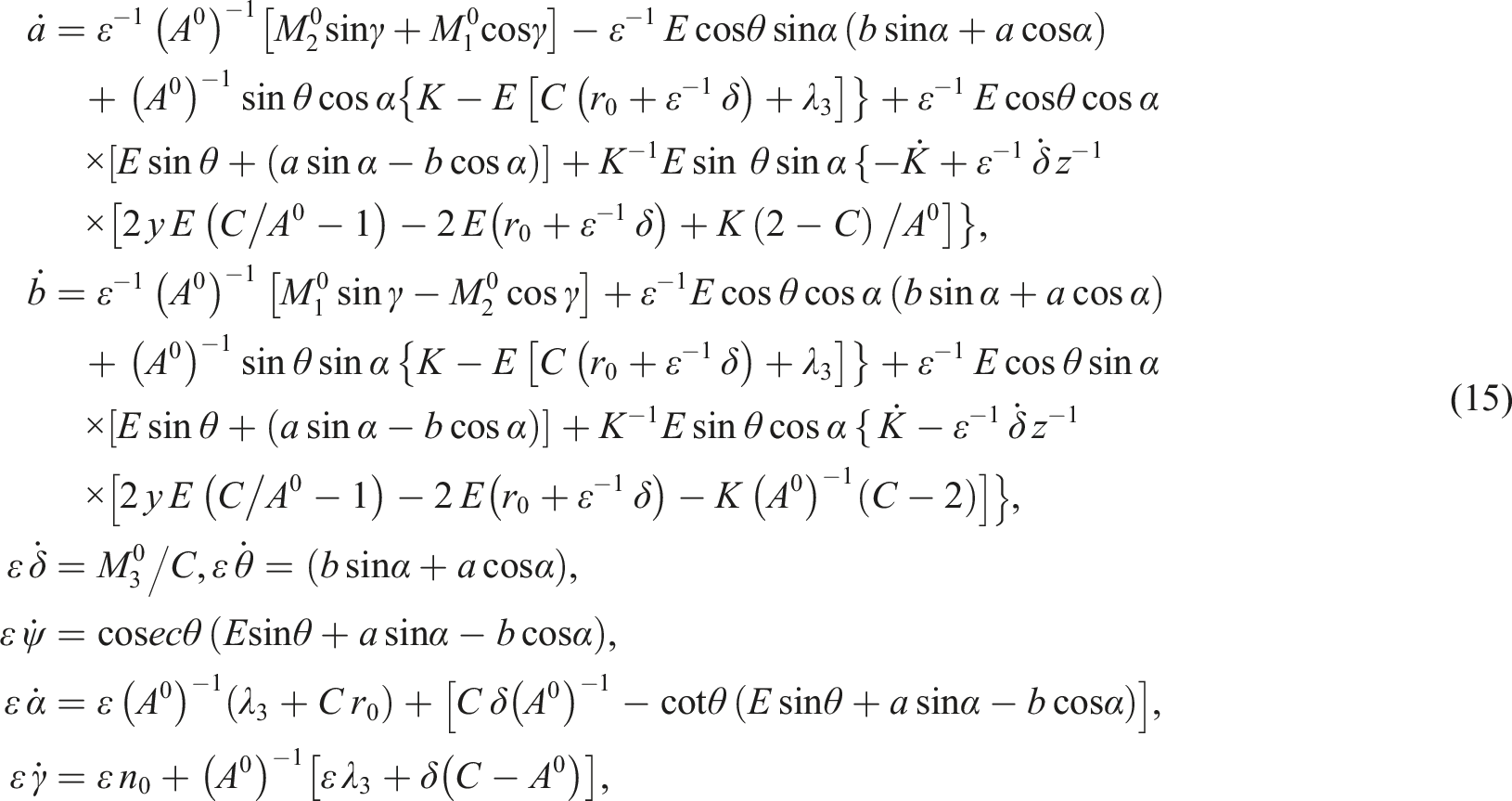
Averaging the considered problem in a suitable manner for ³⁵ and making use of assumptions (4), the restoring torque $K$ becomes

$\left(K-m\hspace{0.17em}g\hspace{0.17em}\ell \right)\hspace{0.17em}{\left(q^2+p^2\right)}^{-1/2}=B^{*}{{\ell }^{\prime }}^2\cos \theta \hspace{0.17em}.$

(6)

Using (1), (2), and (5) into (3), we get

$\begin{array}{l}{A}^0\dot{P}-Q\left[\left(A^0-C\right)\hspace{0.17em}r-{\lambda }_3-{\epsilon }^{-1} {\delta }_1 {\lambda }_3\right]=K{\epsilon }^{-1}\hspace{0.17em}\left[-\left({\delta }_1-\epsilon \right)\hspace{0.17em}\cos \varphi \hspace{0.17em}\sin \theta -y_1\cos \theta \right]\\ +{\epsilon }^{-1} Q r\left[{\delta }_1\left(C-A^0\right)+{\delta }_2{A}^0\right],\\ A^0\dot{Q}-P\left[\left(C-A^0\right)\hspace{0.17em}r+\left(1-{\epsilon }^{-1} {\delta }_2\right) {\lambda }_3\right]=-K{\epsilon }^{-1}\hspace{0.17em}\left[\left(\epsilon -{\delta }_2\right)\sin \varphi \sin \theta -x_1\cos \theta \right]\\ +{\epsilon }^{-1}P r \left[{\delta }_2\left(A^0-C\right)-{\delta }_1{A}^0\right],\\ \dot{r}=-{\epsilon }^{-2}\hspace{0.17em}\left(x_1\cos \varphi -y_1\sin \varphi \right)K\sin \theta /C,\\ \dot{\theta }=-{\epsilon }^{-1} \left(Q \sin \varphi -P \cos \varphi \right),\\ \dot{\varphi }-r=-{\epsilon }^{-1} \cot \theta \left(Q \cos \varphi +P \sin \varphi \right),\\ \dot{\psi }={\epsilon }^{-1} \cos ec\theta \left(Q \cos \varphi +P \sin \varphi \right).\end{array}$

(7)

Recalling (3)–(5), one can write $M_j^{*}$ in the forms

$\begin{array}{l}{M}_1^{*}=-K\left(y_1\cos \theta +{\delta }_1\sin \theta \cos \varphi \right)+Q\left[r\hspace{0.17em}\left({\delta }_1\left(C-A^0\right)-{\delta }_1 {\lambda }_3-{\delta }_2{A}^0\right)\right],\\ M_2^{*}=K\left(x_1\cos \theta +{\delta }_2\sin \theta \sin \varphi \right)+P\left[r\hspace{0.17em}\left({\delta }_2\left(A^0-C\right)+{\delta }_2 {\lambda }_3-{\delta }_1{A}^0\right)\right],\\ M_3^{*}=-K\sin \theta \hspace{0.17em}\left(x_1\cos \varphi -y_1\sin \varphi \right).\end{array}$

(8)

Let $\epsilon \to \infty$ , then (7) gives

$r=r_0,\theta ={\theta }_0,\varphi -{\varphi }_0=r_{0}t,$

(9)

where $r_0,{\theta }_0,$ and ${\phi }_0$ are, respectively, the initial quantities of $r,\theta ,$ and $\phi$ .

Using (7) and (9) to yield

$\begin{array}{l}\ddot{P}+y_0^2 P=E_3\sin \left(r_0 t+{\varphi }_0\right),\\ \ddot{Q}+y_0^2 Q=E_3\cos \left(r_0 t+{\varphi }_0\right),\end{array}$

(10)

where

$\begin{array}{l}\frac{E_3}{z_0}=K_0\sin {\theta }_0,z_0={\left(A^0\right)}^{-1}\left[\left(n_0-r_0\right)+{\left(A^0\right)}^{-1}{\lambda }_3\right],\\ n_0=\left[C{\left(A^0\right)}^{-1}-1\right] r_0,k_0=K_0.\end{array}$

Integrating (10) to obtain

$\begin{array}{l}P-a\cos {\gamma }_0=b\sin {\gamma }_0+E_4\sin \left(r_{0}t+{\varphi }_0\right),\\ Q-a\sin {\gamma }_0=-b\cos {\gamma }_0+E_4\cos \left(r_{0}t+{\varphi }_0\right),\end{array}$

(11)

where

$\begin{array}{l}a=P_0-E_4\sin {\varphi }_0,b=-Q_0+E_4\cos {\varphi }_0,\\ {\gamma }_0/y_0=t,E_4=E_0\sin {\theta }_0,\left|y_0/r_0\right|<1,r_0\ne 0,\\ y_0=n_0+{\left(A^0\right)}^{-1}{\lambda }_3,E_0=z_0 k_0/\left(y_0^2-r_0^2\right),\end{array}$

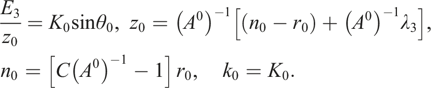
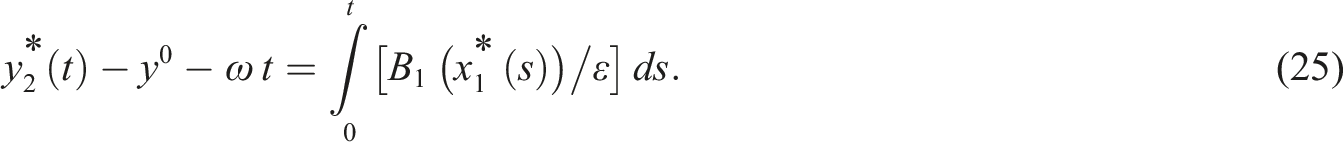
where $P_0,Q_0$ , and $K_0$ are the initial values of the corresponding variables, while $\gamma ={\gamma }_0$ is a phase oscillation. From system (7) we can define

$\dot{\gamma }=y,\gamma \left(0\right)=0,\left(y-n\right)A^0={\lambda }_3,\left(n+r\right)A^0=Cr.$

(12)

We aim to find the solutions of system (7) when $\epsilon \to \infty$ . Using (9), equation (11) can be rewritten in the form

$-\left(\varphi +\gamma \right)={\tan }^{-1}\left(-a+P\cos \gamma +Q\sin \gamma \right)\hspace{0.17em}{\left(b-P\sin \gamma +Q\cos \gamma \right)}^{-1}.$

(13)

The axial component $r$ of angular velocity $\underset{\_}{\omega }$ can be rewritten as follows

$\delta =\epsilon \left(r-r_0\right).$

(14)

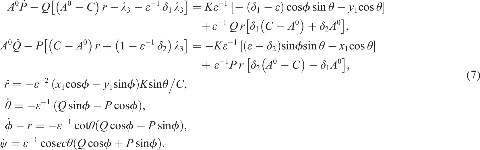
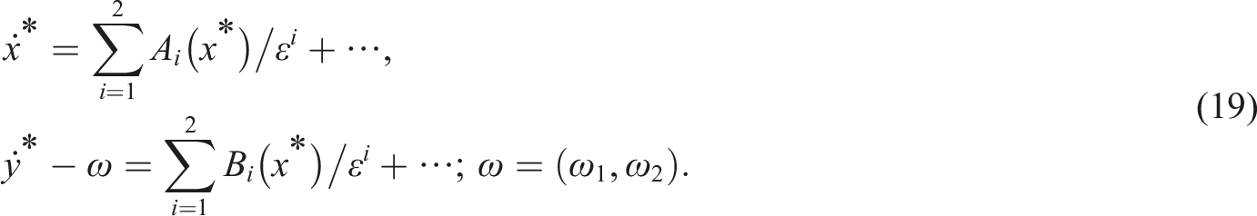
Using (13) and (14) to rewrite (7) and (12) in the form

$\begin{array}{l}\dot{a}={\epsilon }^{-1}\hspace{0.17em}{\left(A^0\right)}^{-1}\left[M_2^0\sin \gamma +M_1^0\cos \gamma \right]-{\epsilon }^{-1}\hspace{0.17em}E\cos \theta \hspace{0.17em}\sin \alpha \hspace{0.17em}\left(b\sin \alpha +a\cos \alpha \right)\\ +{\left(A^0\right)}^{-1}\sin \theta \hspace{0.17em}\cos \alpha \left\{K-E \left[C \left(r_0+{\epsilon }^{-1} \delta \right)+{\lambda }_3\right]\right\}+{\epsilon }^{-1} E \cos \theta \hspace{0.17em}\cos \alpha \\ \times \left[E\sin \theta +\left(a\sin \alpha -b\cos \alpha \right)\right]+K^{-1}E\sin \theta \sin \alpha \hspace{0.17em}\{-\dot{K}+{\epsilon }^{-1} \dot{\delta } z^{-1}\\ \times \left[2 y E \left(C/A^0-1\right)-2 E\left(r_0+{\epsilon }^{-1} \delta \right)+K\hspace{0.17em}\left(2-C\right) /A^0\right]\},\\ \dot{b}={\epsilon }^{-1}\hspace{0.17em}{\left(A^0\right)}^{-1}\hspace{0.17em}\left[M_1^0\hspace{0.17em}\sin \gamma -M_2^0\hspace{0.17em}\cos \gamma \right]+{\epsilon }^{-1}E\cos \theta \hspace{0.17em}\cos \alpha \hspace{0.17em}\left(b\sin \alpha +a\cos \alpha \right)\\ +{\left(A^0\right)}^{-1}\hspace{0.17em}\sin \theta \hspace{0.17em}\sin \alpha \hspace{0.17em}\left\{K-E \left[C \left(r_0+{\epsilon }^{-1} \delta \right)+{\lambda }_3\right]\right\}+{\epsilon }^{-1} E \cos \theta \hspace{0.17em}\sin \alpha \\ \times \left[E\sin \theta +\left(a\sin \alpha -b\cos \alpha \right)\right]+K^{-1}E\sin \theta \hspace{0.17em}\cos \alpha \hspace{0.17em}\{\hspace{0.17em}\dot{K}-{\epsilon }^{-1} \dot{\delta } z^{-1}\\ \times \left[2 y E \left(C/A^0-1\right)-2 E\left(r_0+{\epsilon }^{-1} \delta \right)-K\hspace{0.17em}{\left(A^0\right)}^{-1}\left(C-2\right)\right]\},\\ \epsilon \dot{\delta }=M_3^0/C,\epsilon \dot{\theta }=\left(b \sin \alpha +a \cos \alpha \right),\\ \epsilon \dot{\psi }=\cos ec\theta \hspace{0.17em}\left(E\sin \theta +a \sin \alpha -b \cos \alpha \right),\\ \epsilon \dot{\alpha }=\epsilon \hspace{0.17em}{\left(A^0\right)}^{-1}\left({\lambda }_3+C r_0\right)+\left[C\hspace{0.17em}\delta {\left(A^0\right)}^{-1}-\cot \theta \hspace{0.17em}\left(E \sin \theta +a \sin \alpha -b \cos \alpha \right)\right],\\ \epsilon \dot{\gamma }=\epsilon n_0+{\left(A^0\right)}^{-1}\left[\epsilon {\lambda }_3+\delta \left(C-A^0\right)\right],\end{array}$

(15)

where

$M_j^0\left(a,b,\theta ,\psi ,\alpha ,\gamma ,\delta ,t\right)=M_j^{*}\left(P,Q,r,\theta ,\varphi ,\psi ,t\right),\left(j=1,2,3\right).$

(16)

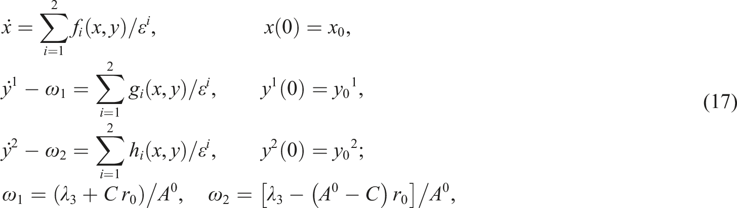
Due to (13), (14), and (16), $M_j^0\left(\alpha ,\gamma \right)$ are periodic functions with a period $2\pi$ . In accordance with (13) and (14), the functions $M_j^0$ are periodic functions of $\alpha$ and $\gamma$ with periods of $2\pi$ . Then, we can rewrite system (15) in a more suitable form

$\begin{array}{l}\dot{x}={\displaystyle \sum }_{i=1}^2{f}_i\left(x,y\right)/{\epsilon }^i,x\left(0\right)=x_0,\\ {\dot{y}}^1-{\omega }_1={\displaystyle \sum }_{i=1}^2{g}_i\left(x,y\right)/{\epsilon }^i,y^1\left(0\right)={y_0}^1,\\ {\dot{y}}^2-{\omega }_2={\displaystyle \sum }_{i=1}^2{h}_i\left(x,y\right)/{\epsilon }^i,y^2\left(0\right)={y_0}^2;\\ {\omega }_1=\left({\lambda }_3+C\hspace{0.17em}{r}_0\right)/A^0,{\omega }_2=\left[{\lambda }_3-\left(A^0-C\right)\hspace{0.17em}{r}_0\right]/A^0,\end{array}$

(17)

where $x=\left(x^1,x^2,\dots ,x^5\right)$ is a vector variable function, $y^1,y^2$ are fast variables functions, and $f_i,g_i,h_i\hspace{0.17em}\left(i=1,2\right)$ are vector-valued functions that can be determined from the right-hand sides (15).

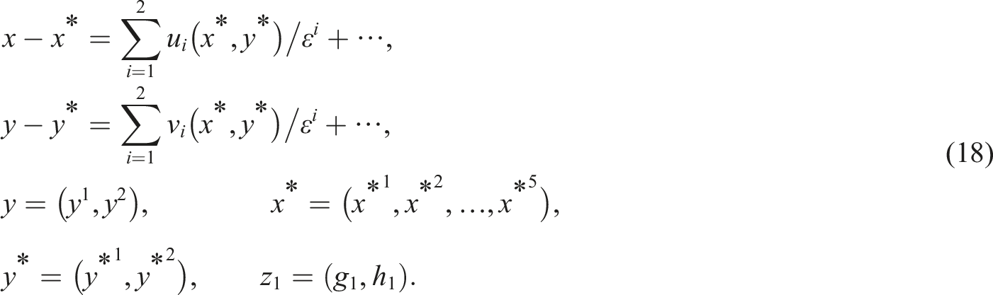
Let $z_1$ denotes the matrix of two-variable vectors $\left(g_1,h_1\right)$ . Then the perturbed torques $M_j^{*}$ are assumed to be independent of $t$ . Introducing new variables for a system (17) as follows ⁴¹

$\begin{array}{l}x-x^{*}={\displaystyle \sum }_{i=1}^2{u}_i\left(x^{*},y^{*}\right)/{\epsilon }^i+\cdots ,\\ y-y^{*}={\displaystyle \sum }_{i=1}^2{v}_i\left(x^{*},y^{*}\right)/{\epsilon }^i+\cdots ,\\ y=\left(y^1,y^2\right),x^{*}=\left({x^{*}}^1,{x^{*}}^2,\dots ,{x^{*}}^5\right),\\ y^{*}=\left({y^{*}}^1,{y^{*}}^2\right),z_1=\left(g_1,h_1\right).\end{array}$

(18)

Then, system (17) can be rewritten for the variable $x^{*}$ and $y^{*}$ as follows

$\begin{array}{l}{\dot{x}}^{*}={\displaystyle \sum }_{i=1}^2{A}_i\left(x^{*}\right)/{\epsilon }^i+\cdots ,\\ {\dot{y}}^{*}-\omega ={\displaystyle \sum }_{i=1}^2{B}_i\left(x^{*}\right)/{\epsilon }^i+\cdots ;\hspace{0.17em}\omega =\left({\omega }_1,{\omega }_2\right).\end{array}$

(19)

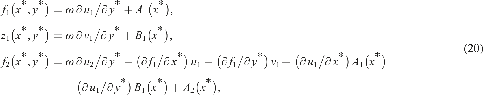
Choosing the vector-valued functions $f_1,z_1,$ and $f_2$ as follows ⁴²

$\begin{array}{l}{f}_1\left(x^{*},y^{*}\right)=\omega \partial u_1/\partial y^{*}+A_1\left(x^{*}\right),\\ z_1\left(x^{*},y^{*}\right)=\omega \partial v_1/\partial y^{*}+B_1\left(x^{*}\right),\\ f_2\left(x^{*},y^{*}\right)=\omega \partial u_2/\partial y^{*}-\left(\partial f_1/\partial x^{*}\right) u_1-\left(\partial f_1/\partial y^{*}\right) v_1\\ +\left(\partial u_1/\partial x^{*}\right) A_1\left(x^{*}\right)+\left(\partial u_1/\partial y^{*}\right)\hspace{0.17em}{B}_1\left(x^{*}\right)+A_2\left(x^{*}\right),\end{array}$

(20)

where

$\begin{array}{l}\underset{0}{\overset{2\pi }{{\displaystyle \int }}}\underset{0}{\overset{2\pi }{{\displaystyle \int }}}{f}_1\left(x^{*},y^{*}\right)\hspace{0.17em}d{y^{*}}^1\hspace{0.17em}d{y^{*}}^2=4\hspace{0.17em}{\pi }^2{A}_1\left(x^{*}\right),\\ \underset{0}{\overset{2\pi }{{\displaystyle \int }}}\underset{0}{\overset{2\pi }{{\displaystyle \int }}}{z}_1\left(x^{*},y^{*}\right)\hspace{0.17em}d{y^{*}}^1\hspace{0.17em}d{y^{*}}^2=4\hspace{0.17em}{\pi }^2{B}_1\left(x^{*}\right),\\ \underset{0}{\overset{2\pi }{{\displaystyle \int }}}\underset{0}{\overset{2\pi }{{\displaystyle \int }}}[f_2\left(x^{*},y^{*}\right)+\left(\partial f_1/\partial x^{*}\right) u_1+\left(\partial f_1/\partial y^{*}\right) v_1-\left(\partial u_1/\partial x^{*}\right) A_1\left(x^{*}\right)\\ -\left(\partial u_1/\partial y^{*}\right) B_1\left(x^{*}\right)] d{y^{*}}^1\hspace{0.17em}d{y^{*}}^2=4\hspace{0.17em}{\pi }^2{A}_2\left(x^{*}\right).\end{array}$

(21)

Here, the partial derivatives of $f_1,u_1,v_1,$ and $u_2$ are treated as the below matrix

$\left[\partial f_s/\partial x^i\right],\left(s=\mathrm{1,2,3,4,5},i=\mathrm{1,2}\right).$

(22)

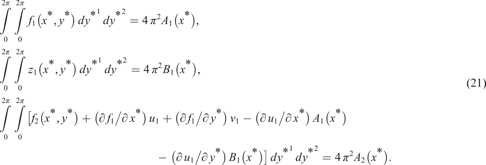
The averaging of the system (19) to determine the slow variables is as follows

$\begin{array}{l}{\dot{x}}_1^{*}=A_1\left(x_1^{*}\right)/\epsilon ,x_1^{*}\left(0\right)=x_{10},\\ {\dot{x}}_2^{*}={\displaystyle \sum }_{i=1}^2{A}_i\left(x_2^{*}\right)/{\epsilon }^i,x_2^{*}\left(0\right)=x_{20}.\end{array}$

(23)

In a similar way, by averaging the system (19), the fast variables can be determined as follows

${\dot{y}}_2^{*}-\omega =B_1\left(x_1^{*}\left(t\right)\right)/\epsilon ,y_2^{*}\left(0\right)=y^0,y^0=\left({y_1}^0,{y_2}^0\right).$

(24)

Integrating (24) to obtain

$y_2^{*}\left(t\right)-y^0-\omega t=\underset{0}{\overset{t}{{\displaystyle \int }}}[B_1\hspace{0.17em}\left(x_1^{*}\hspace{0.17em}\left(s\right)\right)/\epsilon ]\hspace{0.17em}ds.$

(25)

Using $\epsilon \tau =t$ in the system (23), we can get

$d x_2^{*}/d \tau -A_1\hspace{0.17em}\left(x_2^{*}\right)=A_2\left(x_2^{*}\right)/\epsilon .$

(26)

Solving system (26) to yield

$x_2^{*}\left(\tau \right)-x^{\left(1\right)}\left(\tau \right)={\epsilon }^{-1} x^{\left(2\right)}\hspace{0.17em}\left(\tau \right)+O\hspace{0.17em}\left({\epsilon }^{-2}\right).$

(27)

Using (26) and (27), the following system can be obtained

$\begin{array}{l}d x^{\left(1\right)}/d \tau =A_1\left(x^{\left(1\right)}\left(\tau \right)\right),x^{\left(1\right)}\left(0\right)=x_0,\\ d x^{\left(2\right)}/d \tau -A_1^{\prime }\hspace{0.17em}\left(x^{\left(1\right)}\hspace{0.17em}\left(\tau \right)\right)\hspace{0.17em}{x}^{\left(2\right)}=A_2\hspace{0.17em}\left(x^{\left(1\right)}\left(\tau \right)\right),x^{\left(2\right)}\left(0\right)=0.\end{array}$

(28)

Here, $A_1^{\prime }\left(x\right)=\left[\partial {A_1}^i/\partial x^j\right]$ represent a matrix for partial derivatives.

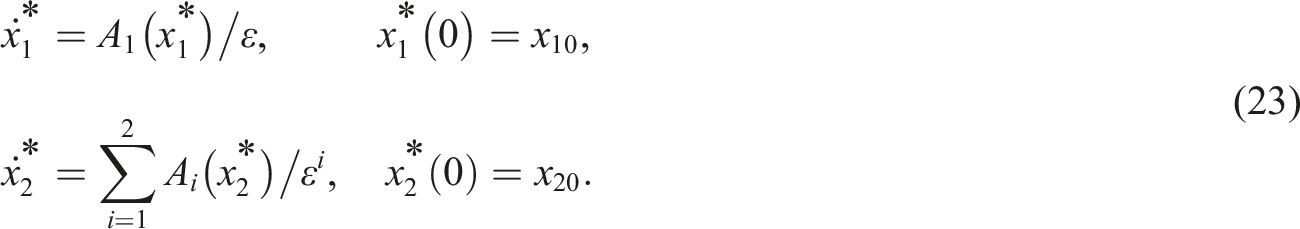
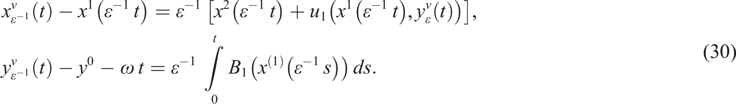
The required solutions for system (28) will be given as follows

$X^{\prime }\left(\tau \right)=A_1\hspace{0.17em}\left(x\right),X\hspace{0.17em}\left(0,c\right)=x_0=c.$

Consequently, functions $x^{\left(1\right)}\hspace{0.17em}\left(\tau \right)$ and $x^{\left(2\right)}\hspace{0.17em}\left(\tau \right)$ can be expressed in forms

$x^{\left(1\right)}\hspace{0.17em}\left(\tau \right)=X\hspace{0.17em}\left(\tau ,x_0\right),x^{\left(2\right)}\left(\tau \right)/\mathrm{\Phi }\left(\tau \right)=\underset{0}{\overset{\tau }{{\displaystyle \int }}}\eta \left(\tau \right)\hspace{0.17em}{\mathrm{\Phi }}^{-1}\left(\tau \right)d\tau ,$

(29)

where

$\mathrm{\Phi }\left(\tau \right)={\left[\partial X\left(\tau ,c\right)/\partial c\right]}_{c=x_0},\eta \left(\tau \right)=A_2\left(X\hspace{0.17em}\left(\tau ,x_0\right)\right).$

The functions $x_{{\epsilon }^{-1}}^{\nu }\left(t\right)$ and $y_{{\epsilon }^{-1}}^{\nu }\left(t\right)$ are vectors and they have the forms

$\begin{array}{l}{x}_{{\epsilon }^{-1}}^{\nu }\left(t\right)-x^1\left({\epsilon }^{-1} t\right)={\epsilon }^{-1}\hspace{0.17em}\left[x^2\left({\epsilon }^{-1} t\right)+u_1\left(x^1\left({\epsilon }^{-1} t\right),y_{\epsilon }^{\nu }\left(t\right)\right)\right],\\ y_{{\epsilon }^{-1}}^{\nu }\left(t\right)-y^0-\omega t={\epsilon }^{-1} \underset{0}{\overset{t}{{\displaystyle \int }}}{B}_1\left(x^{\left(1\right)}\left({\epsilon }^{-1} s\right)\right)\hspace{0.17em}ds.\end{array}$

(30)

By using the Fourier series, equation (20) is solved. From (21), we obtain the function $A_2\left(x^{*}\right)$ . Using (28) and (29), the solutions $x^{\left(1\right)}\left(\tau \right)$ and $x^{\left(2\right)}\left(\tau \right)$ can be obtained. Then the approximated functions $x_{{\epsilon }^{-1}}^{\nu }\left(t\right)$ and $y_{{\epsilon }^{-1}}^{\nu }\left(t\right)$ are constructed according to (30). Now we consider the case of dissipative torques.

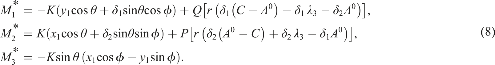
The dissipative torques case

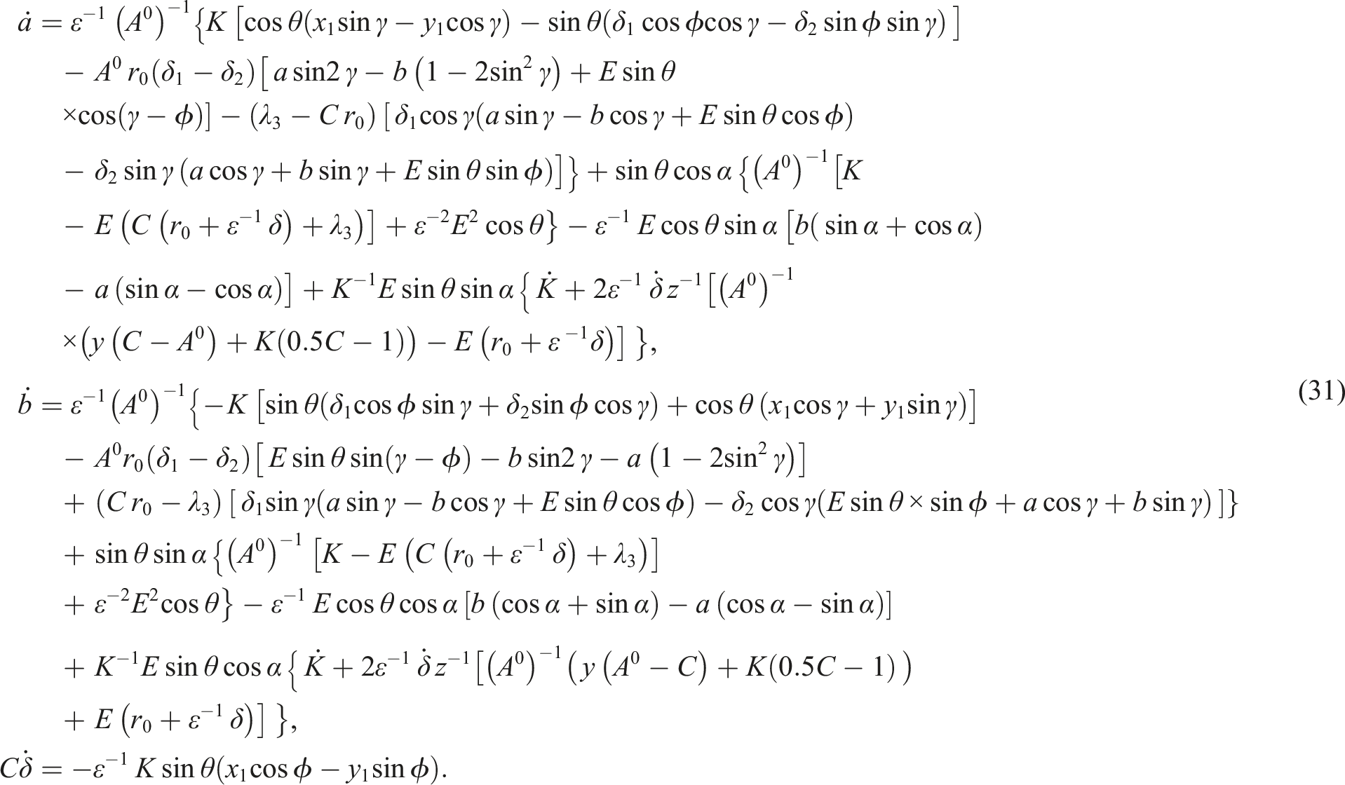
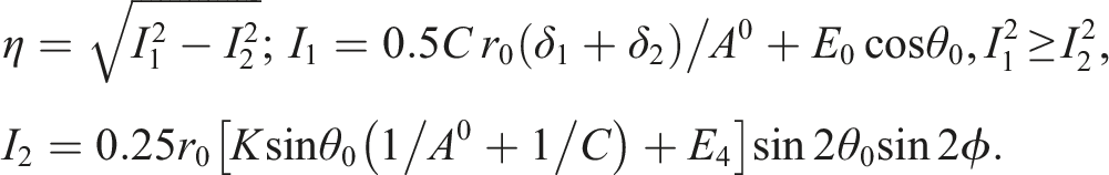
This section presents the averaging procedure to find the required analysis for the angle of nutation $\theta$ and the angle of precession $\psi$ , depending on the large parameter and time. Making use of (6) and (8), then the above three equations of system (15) can be rewritten as follows

$\begin{array}{l}\dot{a}={\epsilon }^{-1} {\left(A^0\right)}^{-1}\{K\hspace{0.17em}[\cos \theta (x_1\sin \gamma -y_1\cos \gamma )-\sin \theta ({\delta }_1\cos \varphi \cos \gamma -{\delta }_2\sin \varphi \sin \gamma )\hspace{0.17em}]\\ -A^0 r_0({\delta }_1-{\delta }_2)[\hspace{0.17em}a\sin 2\gamma -b\hspace{0.17em}(1-2{\sin }^2\gamma )+E\sin \theta \\ \times \cos \left(\gamma -\varphi \right)]-\left({\lambda }_3-C r_0\right) [\hspace{0.17em}{\delta }_1\cos \gamma \left(a\hspace{0.17em}\sin \gamma -b\hspace{0.17em}\cos \gamma +E\sin \theta \cos \varphi \right)\\ -{\delta }_2\hspace{0.17em}\sin \gamma \hspace{0.17em}\left(a\hspace{0.17em}\cos \gamma +b\hspace{0.17em}\sin \gamma +E\sin \theta \sin \varphi \right)\left]\right\}+\sin \theta \cos \alpha \left\{{\left(A^0\right)}^{-1}\right[K\\ -E (C (r_0+{\epsilon }^{-1} \delta )+{\lambda }_3)]+{\epsilon }^{-2}{E}^2\cos \theta \}-{\epsilon }^{-1} E \cos \theta \sin \alpha [b(\hspace{0.17em}\sin \alpha +\cos \alpha )\\ -a\hspace{0.17em}(\sin \alpha -\cos \alpha )]+K^{-1}E\sin \theta \sin \alpha \hspace{0.17em}\{\hspace{0.17em}\dot{K}+2{\epsilon }^{-1} \dot{\delta } z^{-1}[{\left(A^0\right)}^{-1}\\ \times \left(y \left(C-A^0\right)+K\left(0.5C-1\right)\right)-E \left(r_0+\epsilon { }^{-1}\delta \right)]\hspace{0.17em}\},\\ \dot{b}={\epsilon }^{-1}{\left(A^0\right)}^{-1}\{-K\hspace{0.17em}[\sin \theta ({\delta }_1\cos \varphi \sin \gamma +{\delta }_2\sin \varphi \cos \gamma )+\cos \theta \hspace{0.17em}(x_1\cos \gamma +y_1\sin \gamma )]\\ -A^0{r}_0({\delta }_1-{\delta }_2)[\hspace{0.17em}E\sin \theta \sin (\gamma -\varphi )-b\hspace{0.17em}\sin 2\gamma -a\hspace{0.17em}(1-2{\sin }^2\gamma )]\\ +(C r_0-{\lambda }_3) [\hspace{0.17em}{\delta }_1\sin \gamma (a\hspace{0.17em}\sin \gamma -b\hspace{0.17em}\cos \gamma +E\sin \theta \cos \varphi )-{\delta }_2\hspace{0.17em}\cos \gamma (E\sin \theta \times \sin \varphi +a\hspace{0.17em}\cos \gamma +b\hspace{0.17em}\sin \gamma )\hspace{0.17em}]\}\\ +\sin \theta \sin \alpha \{{\left(A^0\right)}^{-1}\hspace{0.17em}[K-E \left(C \left(r_0+{\epsilon }^{-1} \delta \right)+{\lambda }_3\right)]\\ +{\epsilon }^{-2}{E}^2\cos \theta \}-{\epsilon }^{-1} E\cos \theta \cos \alpha \left[b\hspace{0.17em}\left(\cos \alpha +\sin \alpha \right)-a\hspace{0.17em}\left(\cos \alpha -\sin \alpha \right)\right]\\ +K^{-1}E\sin \theta \cos \alpha \hspace{0.17em}\{\hspace{0.17em}\dot{K}+2{\epsilon }^{-1} \dot{\delta } z^{-1}[{\left(A^0\right)}^{-1}( y (A^0-C)+K(0.5C-1)\hspace{0.17em})\\ +E \left(r_0+{\epsilon }^{-1} \delta \right)]\hspace{0.17em}\},\\ C\dot{\delta }=-{\epsilon }^{-1} K\hspace{0.17em}\sin \theta \left(x_1\cos \varphi -y_1\sin \varphi \right).\end{array}$

(31)

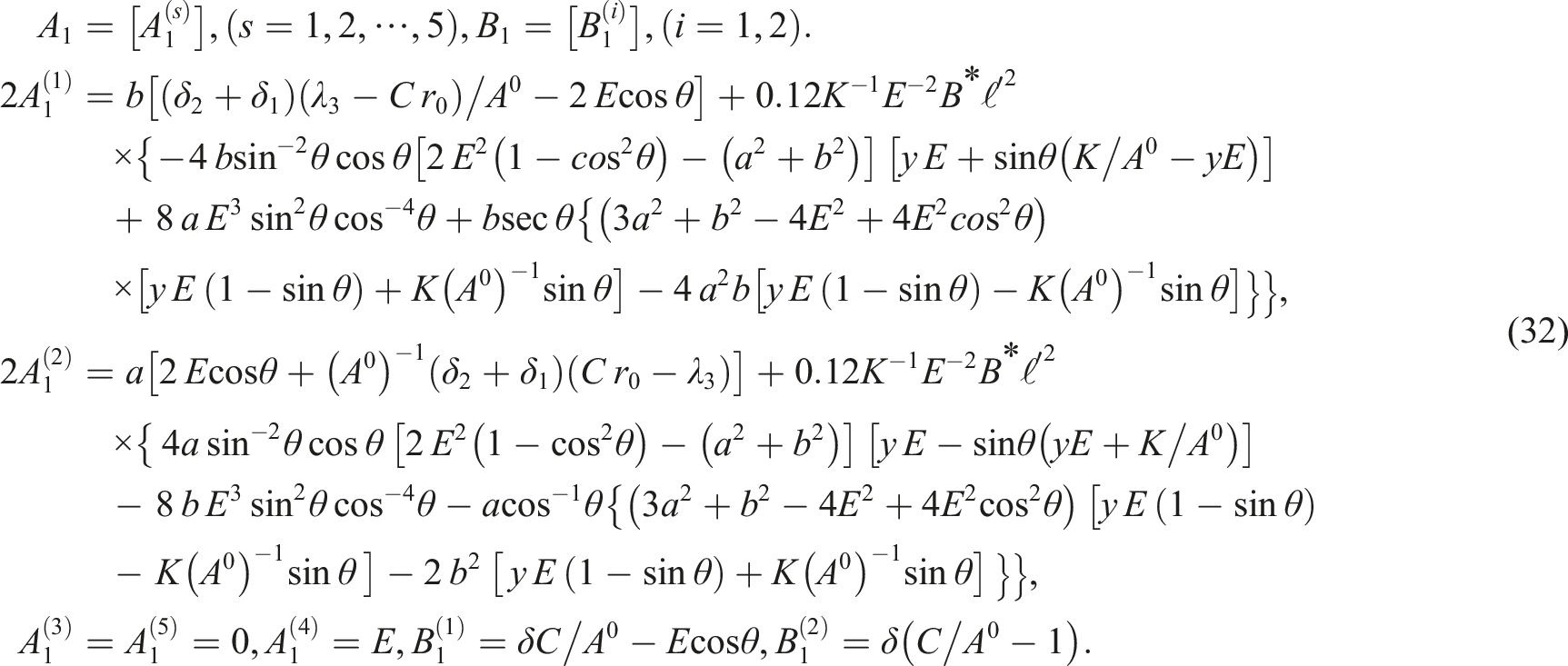
Now, we aim to solve system (31) by applying the averaging technique mentioned above. From (21), one obtains $A_1,B_1$ , and $B_2$ as follows

$\begin{array}{l}{A}_1=\left[A_1^{\left(s\right)}\right],\left(s=1,2,\cdots ,5\right),B_1=\left[B_1^{\left(i\right)}\right],\left(i=1,2\right).\\ 2A_1^{\left(1\right)}=b\left[\left({\delta }_2+{\delta }_1\right)\left({\lambda }_3-C\hspace{0.17em}{r}_0\right)/A^0-2\hspace{0.17em}E\cos \theta \right]+0.12K^{-1}{E}^{-2}{B}^{*}{{\ell }^{\prime }}^2\\ \times \{-4\hspace{0.17em}b{\sin }^{-2}\theta \cos \theta \left[2\hspace{0.17em}{E}^2\left(1-co{\mathrm{s}}^2\theta \right)-\left(a^2+b^2\right)\right] \left[y E+\sin \theta \left(K/A^0-yE\right)\right]\\ +8\hspace{0.17em}a E^3 {\sin }^2\theta {\cos }^{-4}\theta +b\sec \theta \{\left(3a^2+b^2-4E^2+4E^{2}co{\mathrm{s}}^2\theta \right)\\ \times \left[y E \left(1-\sin \theta \right)+K{\left(A^0\right)}^{-1}\sin \theta \right]-4\hspace{0.17em}{a}^{2}b\left[y E \left(1-\sin \theta \right)-K{\left(A^0\right)}^{-1}\sin \theta \right]\left\}\right\},\\ 2A_1^{\left(2\right)}=a\left[2\hspace{0.17em}E\cos \theta +{\left(A^0\right)}^{-1}\left({\delta }_2+{\delta }_1\right)\left(C\hspace{0.17em}{r}_0-{\lambda }_3\right)\right]+0.12K^{-1}{E}^{-2}{B}^{*}{{\ell }^{\prime }}^2\\ \times \{\hspace{0.17em}4a{\sin }^{-2}\theta \cos \theta \hspace{0.17em}\left[2\hspace{0.17em}{E}^2\left(1-{\cos }^2\theta \right)-\left(a^2+b^2\right)\right] \left[y E-\sin \theta \left(yE+K/A^0\right)\right]\\ -8\hspace{0.17em}b\hspace{0.17em}{E}^3 {\sin }^2\theta {\cos }^{-4}\theta -a{\cos }^{-1}\theta \{\left(3a^2+b^2-4E^2+4E^2{\cos }^2\theta \right) [y E \left(1-\sin \theta \right)\\ -K{\left(A^0\right)}^{-1}\sin \theta ]-2\hspace{0.17em}{b}^2\hspace{0.17em}[\hspace{0.17em}y E \left(1-\sin \theta \right)+K{\left(A^0\right)}^{-1}\sin \theta ]\hspace{0.17em}\}\},\\ A_1^{\left(3\right)}=A_1^{\left(5\right)}=0,A_1^{\left(4\right)}=E,B_1^{\left(1\right)}=\delta C/A^0-E\cos \theta ,B_1^{\left(2\right)}=\delta \left(C/A^0-1\right).\end{array}$

(32)

$\begin{array}{l}16K{A}_2^{\left(1\right)}=b B^{*}{{\ell }^{\prime }}^2{E}^{-1} \left[\chi +{\chi }_1\left(5a^2+b^2\right)\right],\\ -16K{A}_2^{\left(2\right)}=a B^{*}{{\ell }^{\prime }}^2{E}^{-1}\left[\chi +{\chi }_1\left(a^2+5b^2\right)\right],A_2^{\left(3\right)}=A_2^{\left(5\right)}=0,\\ A_2^{\left(4\right)}=K\delta \left(C-2A^0\right)/\left[\left(C^2-2A^0\right)\left(r_0+\delta \right)+\left(1+2\hspace{0.17em}{A}^0\right)\hspace{0.17em}{\lambda }_3^2\right],\\ \chi =4E^3{\sin }^3\theta \left(1+{\sec }^2\theta \right)+2\cos \theta \hspace{0.17em}\left({\sec }^2\theta -3\right)\left(\delta +E\cos \theta \right)\\ -\left(a^2+b^2\right){\sin }^{-2}\theta \hspace{0.17em}\left[1+2\hspace{0.17em}\cos \theta \left(E^{-1}\delta +\cos \theta \right)-E\hspace{0.17em}\left(3+{\sec }^2\theta \right){\sin }^3\theta \right]\\ {\chi }_1=-0.5\left(1+E^{-1}\delta \sec \theta \right).\end{array}$

(33)

The solution of system (31) gives

$\begin{array}{l}{a}^{\left(1\right)}={\chi }_2+{\chi }_3,b^{\left(1\right)}={\varphi }_0-a^{\left(1\right)}+Q_0\sin \eta t,{\psi }^{\left(1\right)}={\psi }_0+{\epsilon }^{-1}{E}_0 t,\\ A^0{\gamma }^{\left(1\right)}=\left[\left(C-A^0\right)\hspace{0.17em}{r}_0+{\lambda }_3\right] t,{\alpha }^{\left(1\right)}=C{r}_0/A^0+{\varphi }_0+\left[{\lambda }_3/A^0-E_0\cos {\theta }_0\right]\hspace{0.17em}t,\\ {\theta }^{\left(1\right)}={\theta }_0,{\chi }_2=P_0\cot \eta t+{\varphi }_0\hspace{0.17em}{\chi }_3=Q_0\sin \eta t-E_4\sin \eta t,\end{array}$

(34)

where

$\begin{array}{l}\eta =\sqrt{I_1^2-I_2^2};\hspace{0.17em}{I}_1=0.5C r_0\left({\delta }_1+{\delta }_2\right)/A^0+E_0\cos {\theta }_0,I_1^2\ge I_2^2,\\ I_2=0.25r_0\left[K\sin {\theta }_0\left(1/A^0+1/C\right)+E_4\right]\sin 2{\theta }_0\sin 2\varphi .\end{array}$

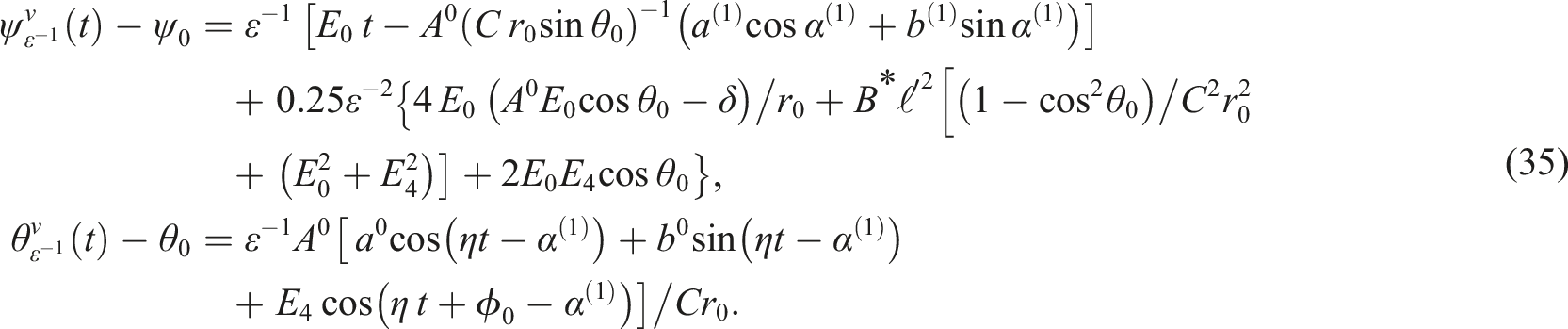
Using equations (30), and (32)–(34), we obtain Euler’s angles $\psi$ and $\theta$ corresponding to the functional components $x_{{\epsilon }^{-1}}^{\nu }\left(t\right)$ for the case of the dissipative torque (8), as follows

$\begin{array}{l}{\psi }_{{\epsilon }^{-1}}^{\nu }\left(t\right)-{\psi }_0={\epsilon }^{-1} \left[E_0\hspace{0.17em}t-A^0{\left(C\hspace{0.17em}{r}_0\sin {\theta }_0\right)}^{-1}\left(a^{\left(1\right)}\cos \hspace{0.17em}{\alpha }^{\left(1\right)}+b^{\left(1\right)}\sin {\alpha }^{\left(1\right)}\right)\right]\\ +0.25{\epsilon }^{-2}\{4 E_0 \left(A^0{E}_0\cos {\theta }_0-\delta \right)/r_0+B^{*}{{\ell }^{\prime }}^2[\left(1-{\cos }^2{\theta }_0\right)/C^2{r}_0^2\\ +\left(E_0^2+E_4^2\right)]+2E_0{E}_4\cos {\theta }_0\},\\ {\theta }_{{\epsilon }^{-1}}^{\nu }\left(t\right)-{\theta }_0={\epsilon }^{-1}{A}^0[\hspace{0.17em}{a}^0\cos \left(\eta t-{\alpha }^{\left(1\right)}\right)+b^0\sin \left(\eta t-{\alpha }^{\left(1\right)}\right)\\ +E_4\cos \left(\eta t+{\varphi }_0-{\alpha }^{\left(1\right)}\right)]/C{r}_0.\end{array}$

(35)

Interpretation of the results

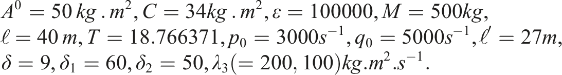
This section presents a discussion of the attained solutions which were mentioned before by intensive programs and studies the influence of changing the parameters of the motion on the solutions. Therefore, consider the next set of data

$\begin{array}{l}{A}^0=50\hspace{0.17em}kg\hspace{0.17em}.\hspace{0.17em}{m}^2,C=34kg\hspace{0.17em}.\hspace{0.17em}{m}^2,\epsilon =100000,M=500kg,\\ \ell =40\hspace{0.17em}m,T=18.766371,p_0=3000s^{-1},q_0=5000s^{-1},{\ell }^{\prime }=27m,\\ \delta =9,{\delta }_1=60,{\delta }_2=50,{\lambda }_3\left(=\mathrm{200,100}\right)kg.m^2.s^{-1}.\end{array}$

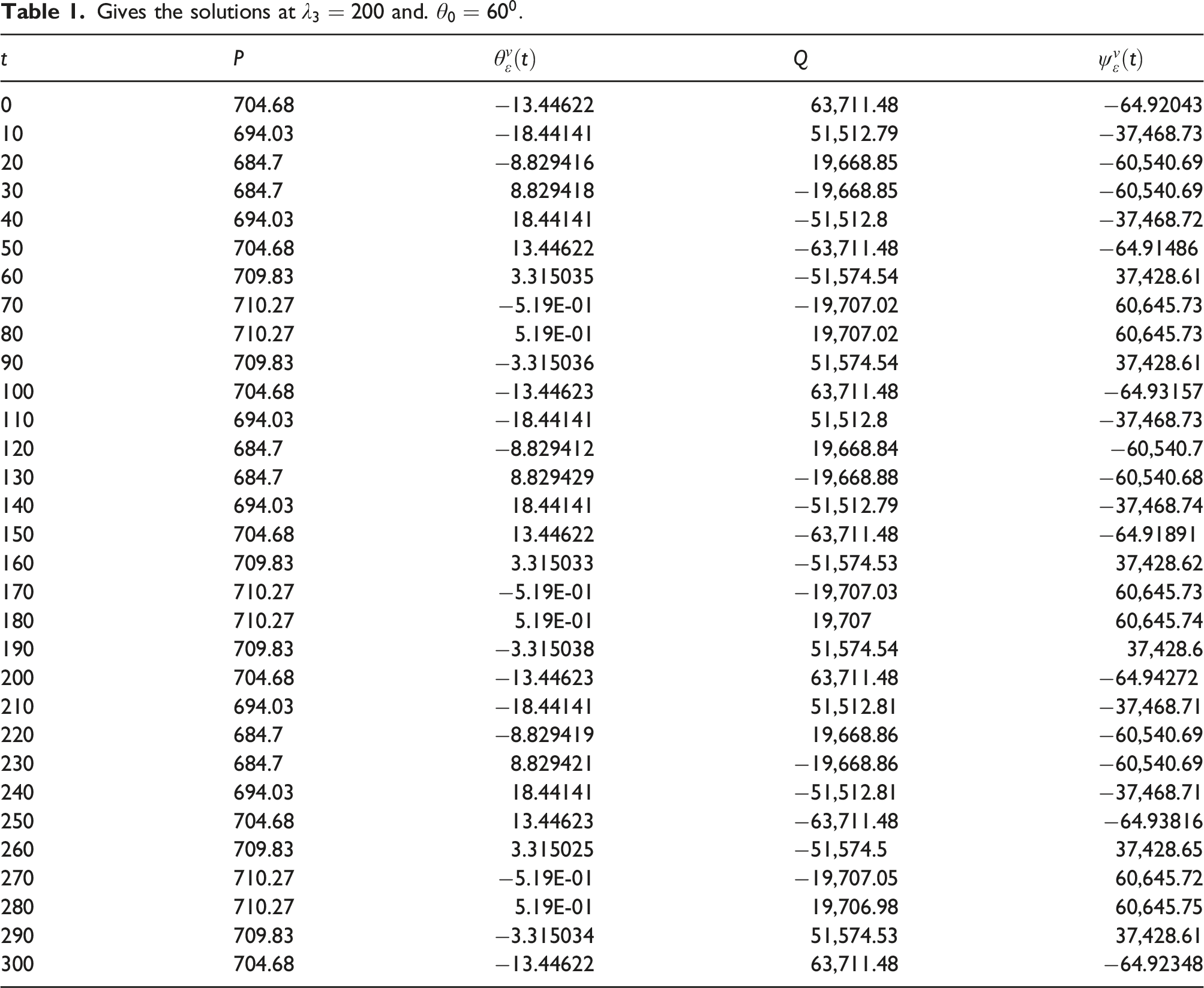
Through a computer program, we represent the numerical results of ${\psi }_{\epsilon }^{\nu }\left(t\right)$ and ${\theta }_{\epsilon }^{\nu }\left(t\right)$ mentioned in previous sections, as in Tables 1 and 2

Table 1.

Gives the solutions at ${\lambda }_3=200$ and. ${\theta }_0={60}^0.$

$t$	$P$	${\theta }_{\epsilon }^{\nu }\left(t\right)$	$Q$	${\psi }_{\epsilon }^{\nu }\left(t\right)$
0	704.68	−13.44622	63,711.48	−64.92043
10	694.03	−18.44141	51,512.79	−37,468.73
20	684.7	−8.829416	19,668.85	−60,540.69
30	684.7	8.829418	−19,668.85	−60,540.69
40	694.03	18.44141	−51,512.8	−37,468.72
50	704.68	13.44622	−63,711.48	−64.91486
60	709.83	3.315035	−51,574.54	37,428.61
70	710.27	−5.19E-01	−19,707.02	60,645.73
80	710.27	5.19E-01	19,707.02	60,645.73
90	709.83	−3.315036	51,574.54	37,428.61
100	704.68	−13.44623	63,711.48	−64.93157
110	694.03	−18.44141	51,512.8	−37,468.73
120	684.7	−8.829412	19,668.84	−60,540.7
130	684.7	8.829429	−19,668.88	−60,540.68
140	694.03	18.44141	−51,512.79	−37,468.74
150	704.68	13.44622	−63,711.48	−64.91891
160	709.83	3.315033	−51,574.53	37,428.62
170	710.27	−5.19E-01	−19,707.03	60,645.73
180	710.27	5.19E-01	19,707	60,645.74
190	709.83	−3.315038	51,574.54	37,428.6
200	704.68	−13.44623	63,711.48	−64.94272
210	694.03	−18.44141	51,512.81	−37,468.71
220	684.7	−8.829419	19,668.86	−60,540.69
230	684.7	8.829421	−19,668.86	−60,540.69
240	694.03	18.44141	−51,512.81	−37,468.71
250	704.68	13.44623	−63,711.48	−64.93816
260	709.83	3.315025	−51,574.5	37,428.65
270	710.27	−5.19E-01	−19,707.05	60,645.72
280	710.27	5.19E-01	19,706.98	60,645.75
290	709.83	−3.315034	51,574.53	37,428.61
300	704.68	−13.44622	63,711.48	−64.92348

Table 2.

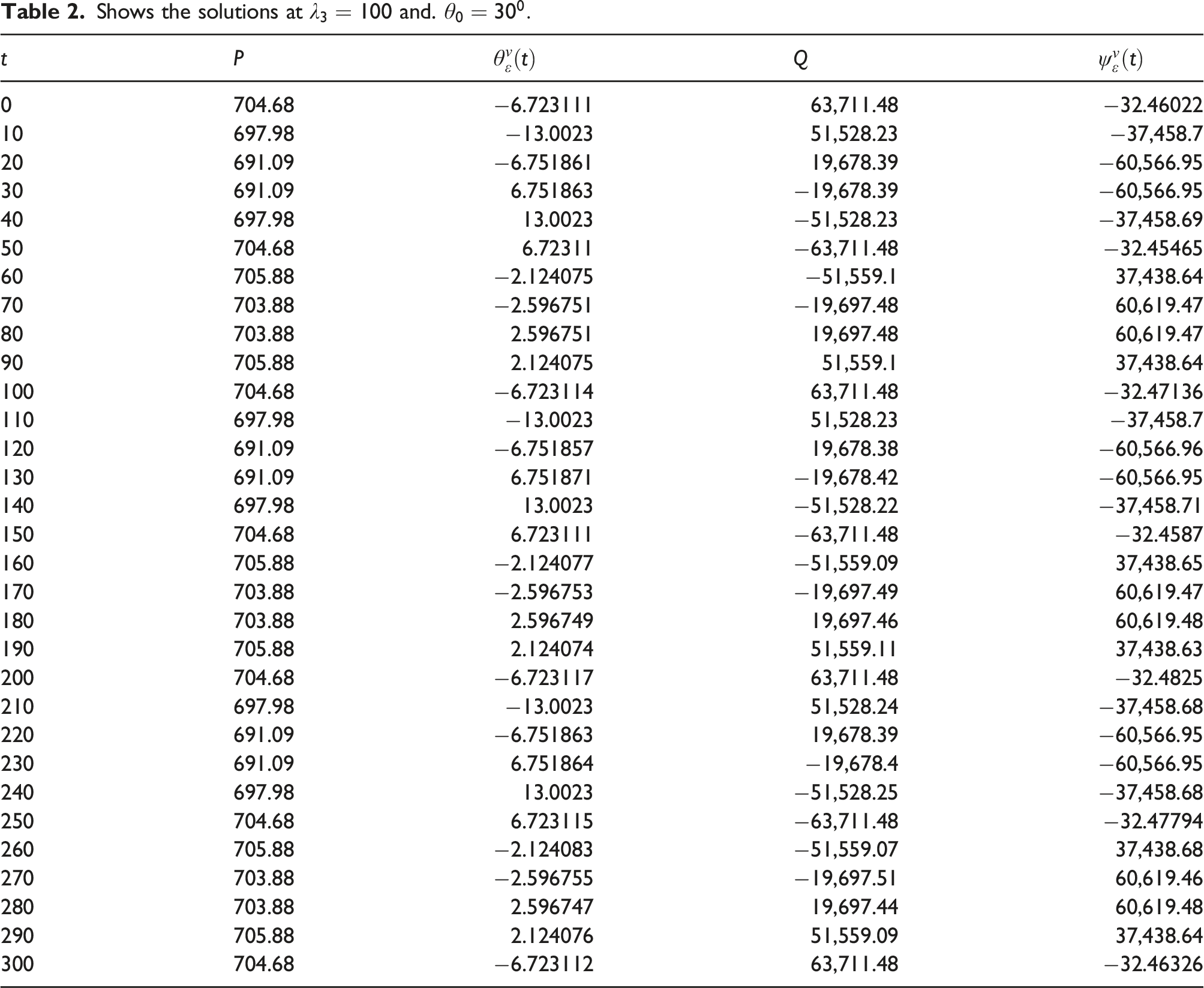
Shows the solutions at ${\lambda }_3=100$ and. ${\theta }_0={30}^0.$

$t$	$P$	${\theta }_{\epsilon }^{\nu }\left(t\right)$	$Q$	${\psi }_{\epsilon }^{\nu }\left(t\right)$
0	704.68	−6.723111	63,711.48	−32.46022
10	697.98	−13.0023	51,528.23	−37,458.7
20	691.09	−6.751861	19,678.39	−60,566.95
30	691.09	6.751863	−19,678.39	−60,566.95
40	697.98	13.0023	−51,528.23	−37,458.69
50	704.68	6.72311	−63,711.48	−32.45465
60	705.88	−2.124075	−51,559.1	37,438.64
70	703.88	−2.596751	−19,697.48	60,619.47
80	703.88	2.596751	19,697.48	60,619.47
90	705.88	2.124075	51,559.1	37,438.64
100	704.68	−6.723114	63,711.48	−32.47136
110	697.98	−13.0023	51,528.23	−37,458.7
120	691.09	−6.751857	19,678.38	−60,566.96
130	691.09	6.751871	−19,678.42	−60,566.95
140	697.98	13.0023	−51,528.22	−37,458.71
150	704.68	6.723111	−63,711.48	−32.4587
160	705.88	−2.124077	−51,559.09	37,438.65
170	703.88	−2.596753	−19,697.49	60,619.47
180	703.88	2.596749	19,697.46	60,619.48
190	705.88	2.124074	51,559.11	37,438.63
200	704.68	−6.723117	63,711.48	−32.4825
210	697.98	−13.0023	51,528.24	−37,458.68
220	691.09	−6.751863	19,678.39	−60,566.95
230	691.09	6.751864	−19,678.4	−60,566.95
240	697.98	13.0023	−51,528.25	−37,458.68
250	704.68	6.723115	−63,711.48	−32.47794
260	705.88	−2.124083	−51,559.07	37,438.68
270	703.88	−2.596755	−19,697.51	60,619.46
280	703.88	2.596747	19,697.44	60,619.48
290	705.88	2.124076	51,559.09	37,438.64
300	704.68	−6.723112	63,711.48	−32.46326

From Tables 1 and 2, we get the approximated solutions ${\psi }_{\epsilon }^{\nu }\left(t\right)$ when ${\lambda }_3\left(=\mathrm{200,100}\right)$ and ${\theta }_0\left(={60}^0,{30}^0\right)$ . From these tables, we deduce that the amplitude of the motion increases when ${\lambda }_3$ and ${\theta }_0$ decrease and vice versa. We also discover that, while the amplitude of the motion increases, the number of oscillations remains constant. We conclude that the number of oscillations of the gyro about the $Z$ -axis remains the same for increasing or decreasing both the third component torque ${\lambda }_3$ and the initial nutation angle ${\theta }_0$ , with different amplitudes of the motion about this axis. Moreover, from Tables 1 and 2, we observe that the amplitude of the approximated solutions ${\theta }_{\epsilon }^{\nu }\left(t\right)$ decreases when ${\lambda }_3$ and ${\theta }_0$ decreases and vice versa. That is the change of ${\theta }_{\epsilon }^{\nu }\left(t\right)$ describes the orientation for a gyro at every point in time $t$ .

Numerical procedure

This section presents a numerical procedure named the method of Runge–Kutta of fourth order applying a computer discussion to solve a system (10). One aims to find the required periodic solutions of $P$ and $Q$ . To achieve this objective, let us consider the values $B^{*}=10\hspace{0.17em}kg.{\left(Amper\right)}^{-1}.s^{-2},\ell =40m,{\theta }_0\left(={60}^0,{30}^0\right),$ and the considered data in the previous section.

Introducing the above data and using the mentioned numerical method with a computer procedure to get numerical results of $P$ and $Q$ via time $t$ , as in Tables 1 and 2 for different values of the torque ${\lambda }_3\left(=200,100\right)$ and ${\theta }_0\left(={60}^0,{30}^0\right)$ . We note that the amplitudes of the motion increase with decreasing of ${\lambda }_3$ and ${\theta }_0$ , and vice versa. We also note that the number of oscillations of the gyro is the same with different amplitudes of the motion, see Tables 1 and 2.

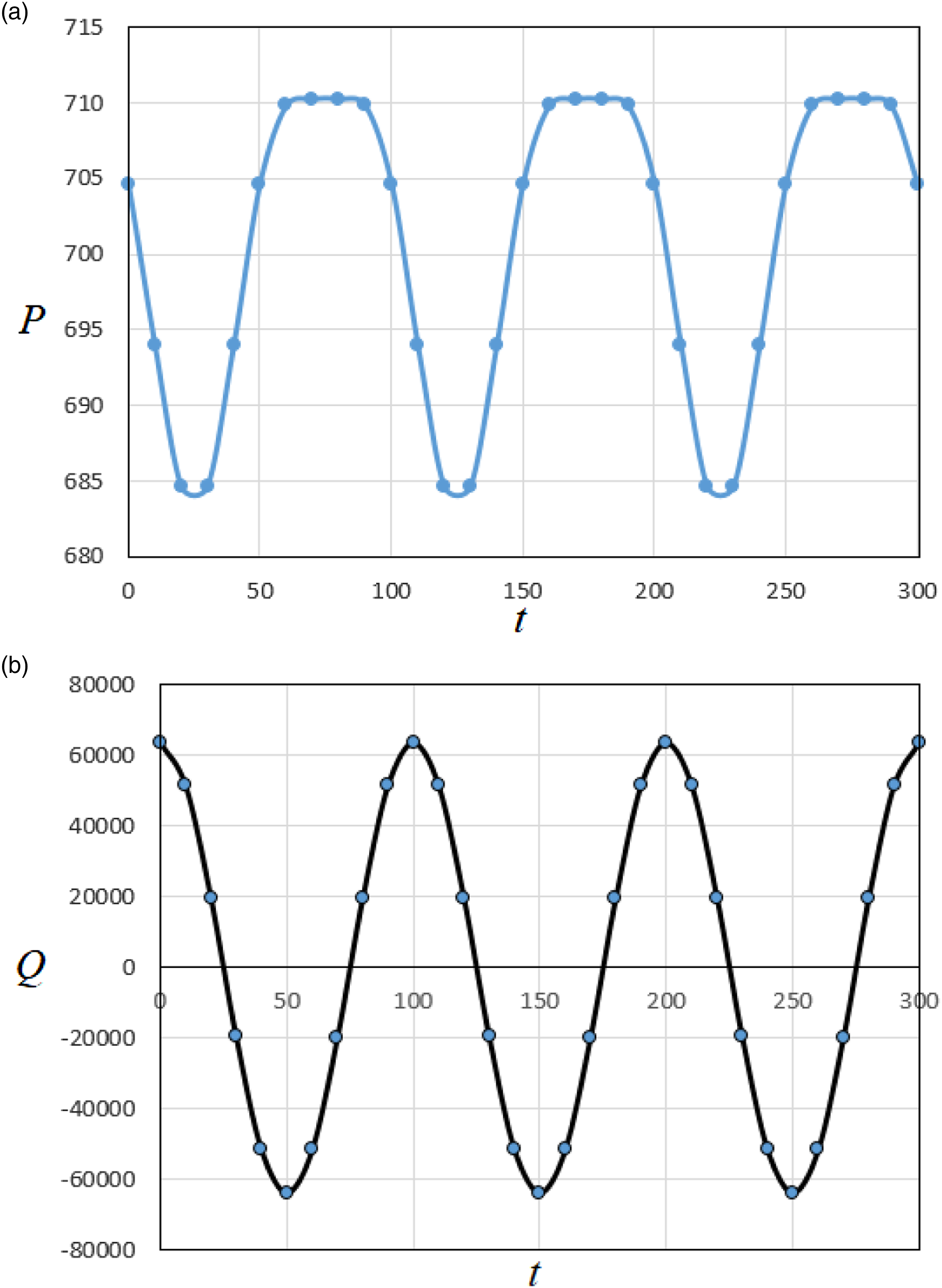
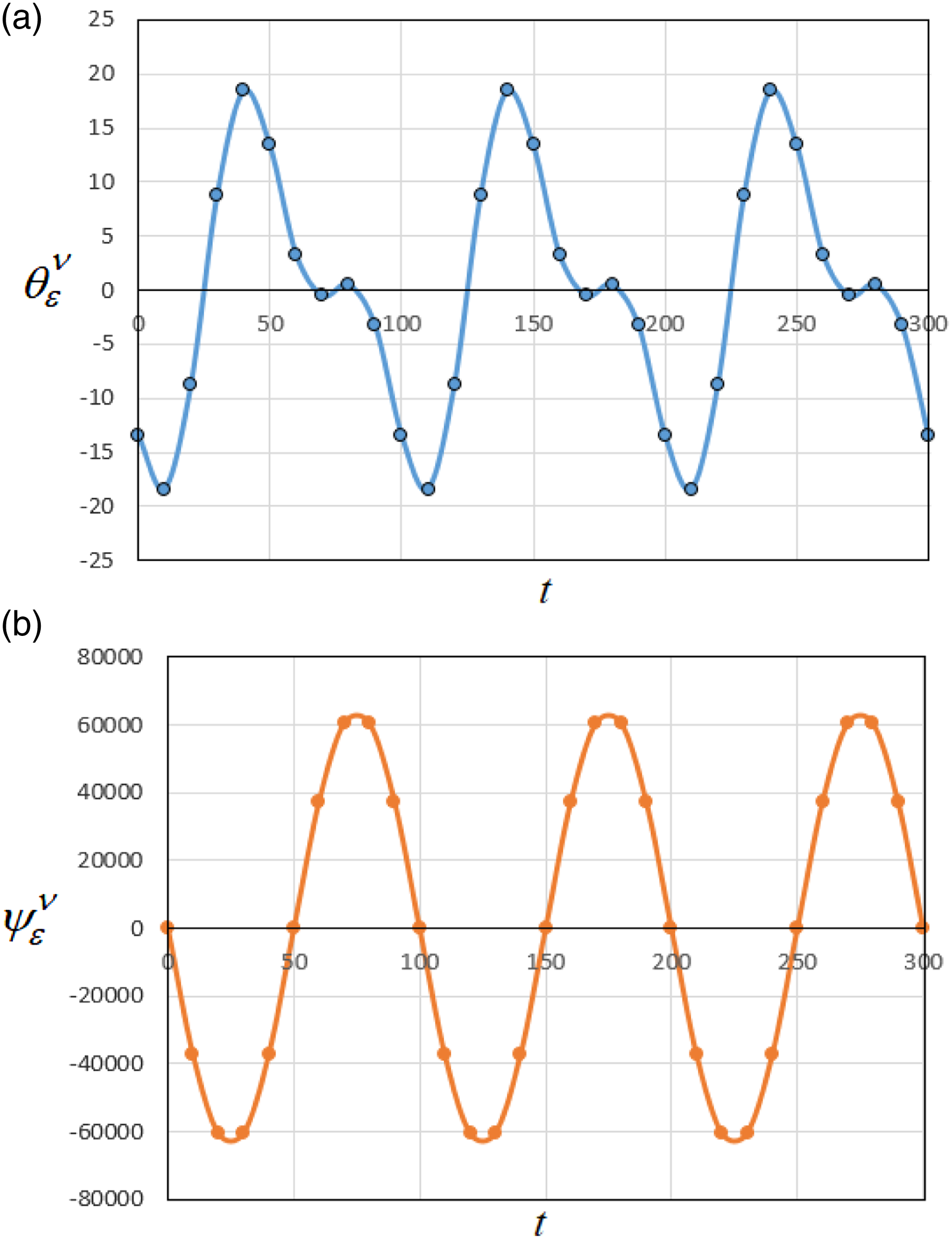
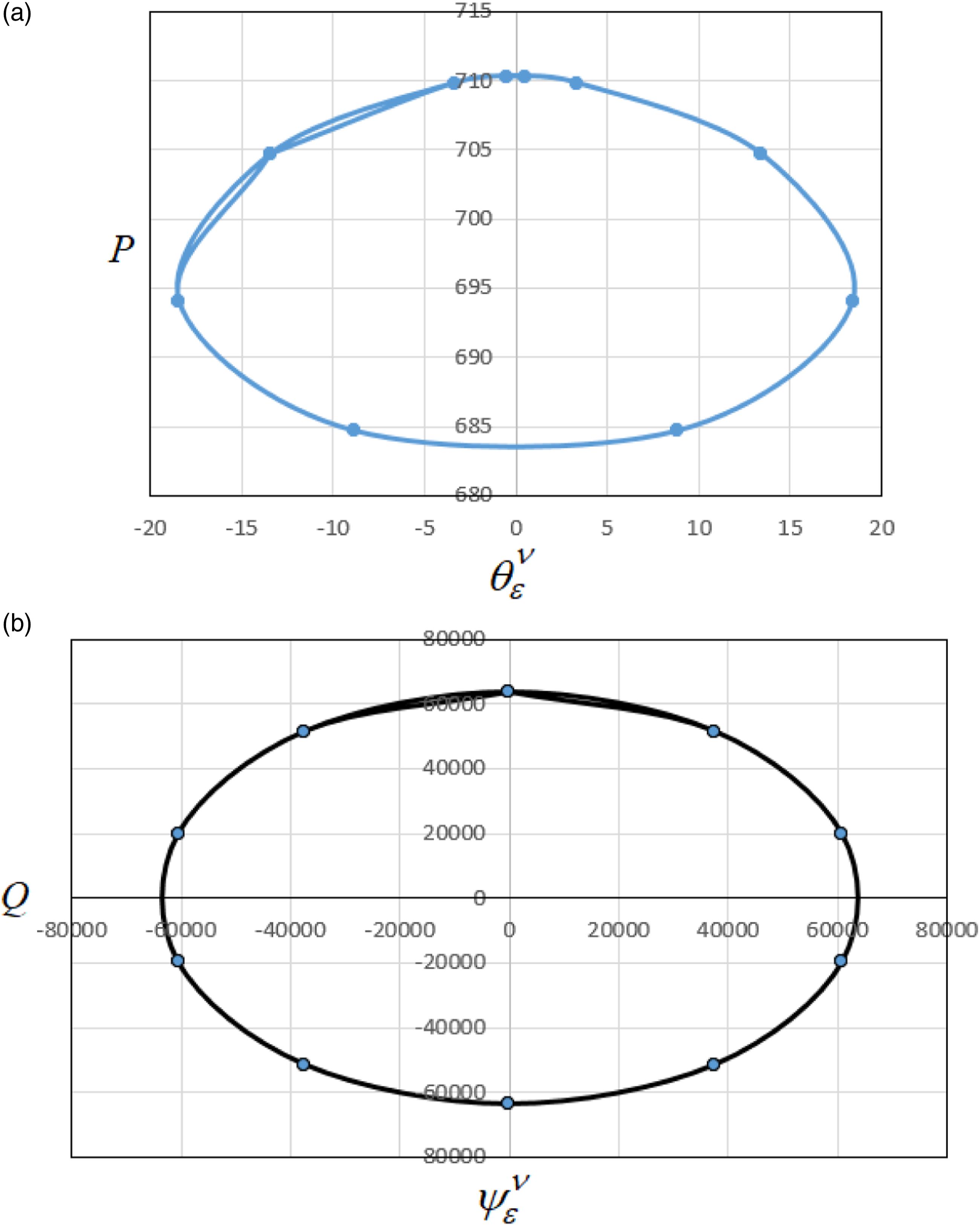
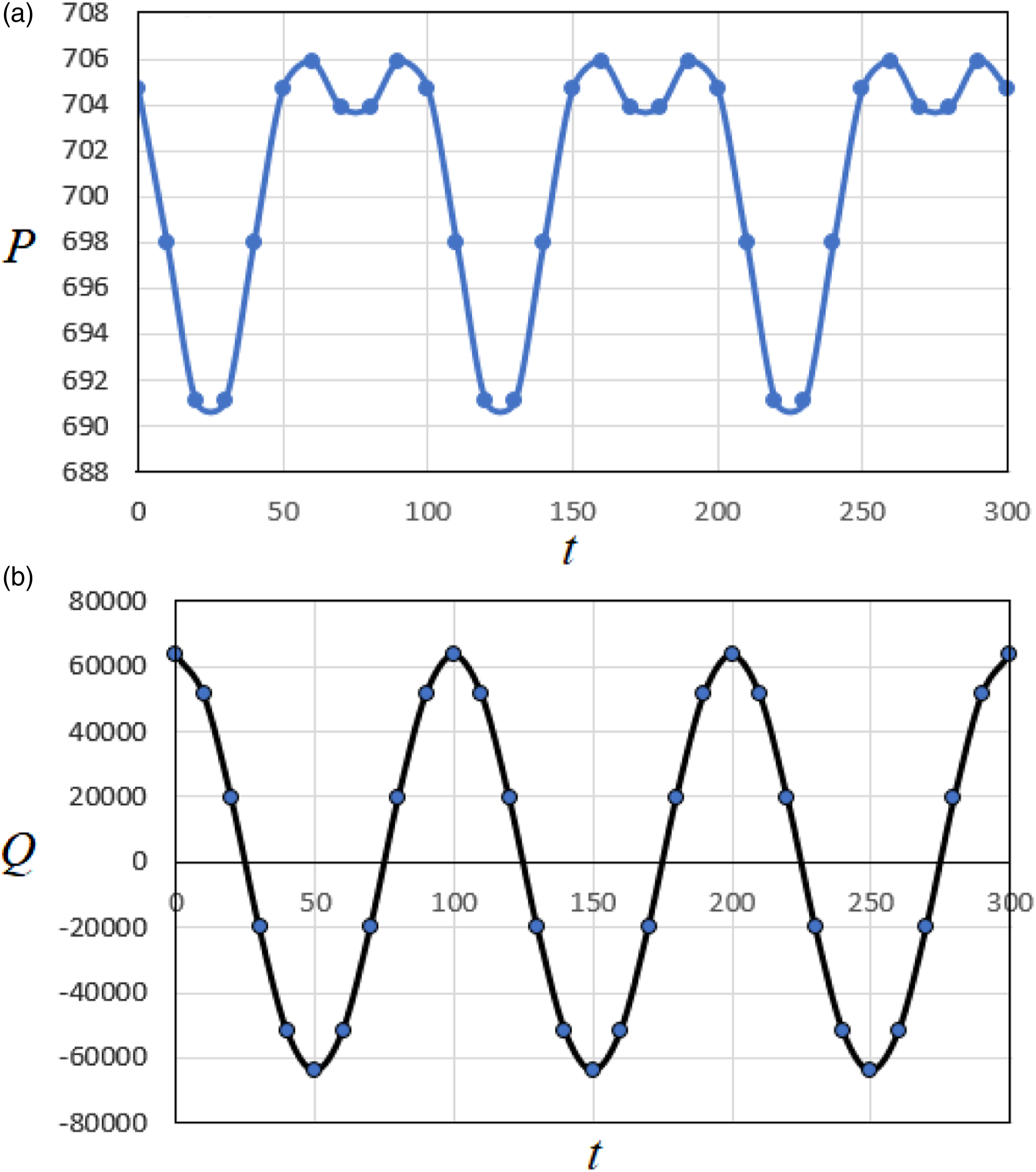
The included results in Table 1 have been plotted in Figures 1–3 to show how the gyro’s motion behaves. The time histories of $P,Q$ and ${\theta }_{\epsilon }^{\nu },{\psi }_{\epsilon }^{\nu }$ are depicted according to the curves in these figures, in which they exhibit periodic behavior, where the displayed curves in portions (a) have substantially smaller amplitudes than the depicted curves in portions (b). It can be seen in Figure 2(a) that waves exhibit closer data at the top of the represented wave, whereas the drawn curves in other portions of these figures exhibit entirely periodic curves throughout the period studied. Parts (a) and (b) of the Figure 3 show the projections of these curves in the planes ${\theta }_{\epsilon }^{\nu }P$ and ${\psi }_{\epsilon }^{\nu }Q$ , which take the shape of closed curves and convey the stability of the gyro’s motion.

Figure 1.

Presents the curves of the results in Table 1: (a) $P\left(t\right)$ , (b) $Q\left(t\right)$ .

Figure 2.

Portrays the curves of the results in Table 1: (a) ${\theta }_{\epsilon }^{\nu }\left(t\right)$ , (b) ${\psi }_{\epsilon }^{\nu }\left(t\right)$ .

Figure 3.

Explores the curves of the results in Table 1: (a) in the plane ${\theta }_{\epsilon }^{\nu }P$ , (b) in the plane ${\psi }_{\epsilon }^{\nu }Q$ .

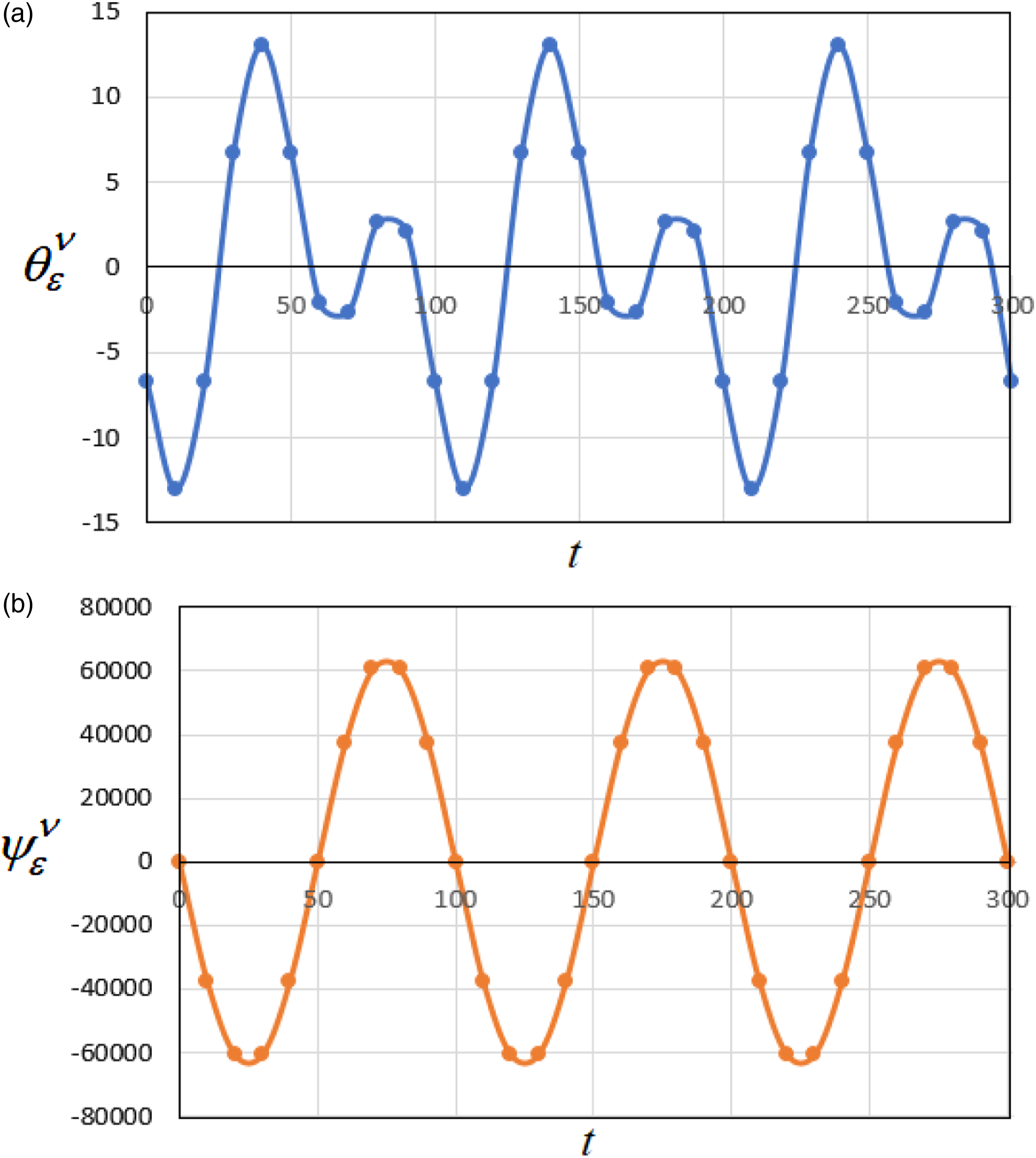
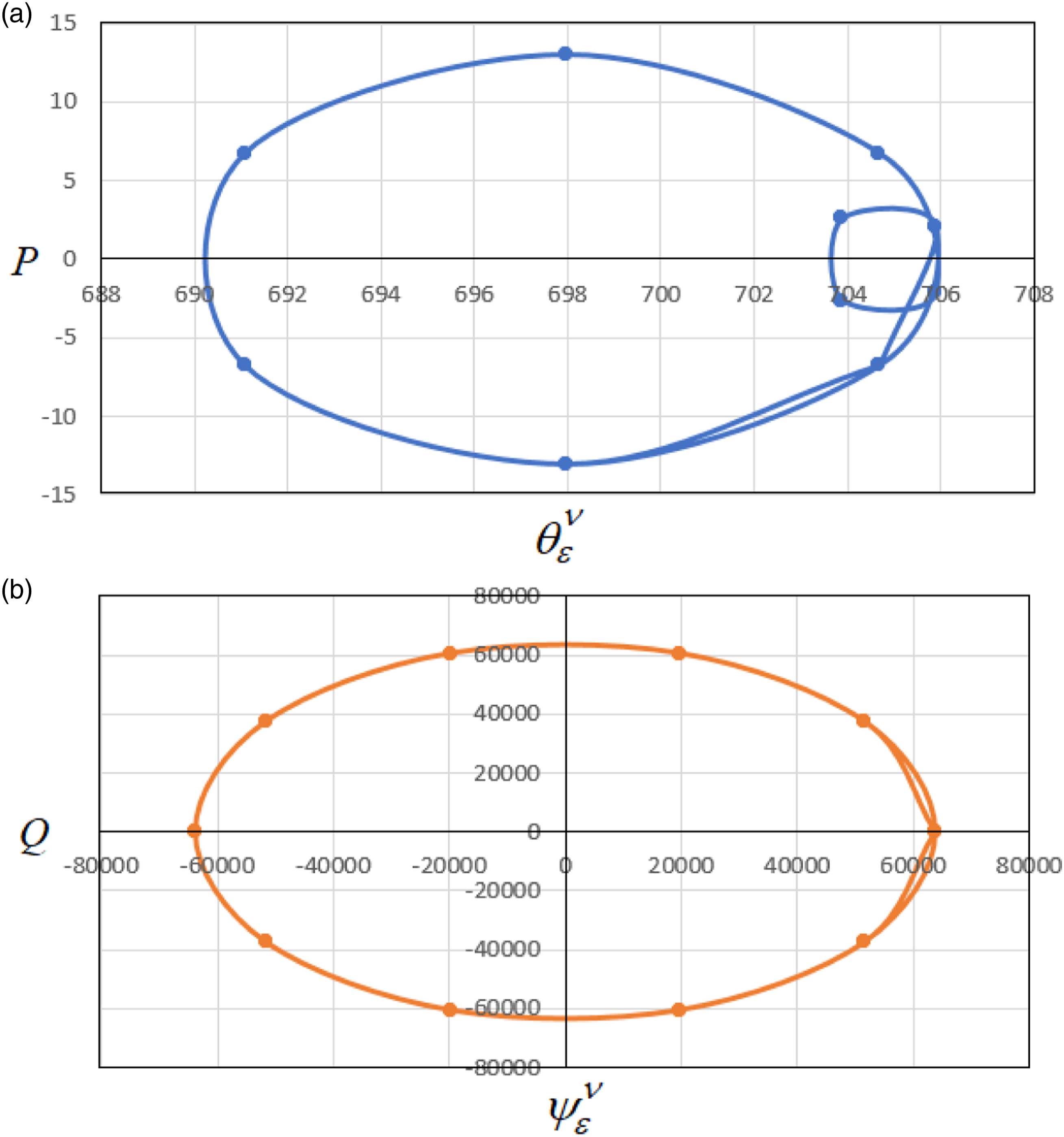
The considered results in Table 2 have been graphed in Figures 4–6, to reveal the behavior of the gyro’s motion. Curves of Figures 4 and 5 show the time histories of $P,Q$ and ${\theta }_{\epsilon }^{\nu },{\psi }_{\epsilon }^{\nu }$ . They have periodic behavior, in which the amplitudes of the presented curves in portions (a) are much less than the plotted curves of parts (b). It is observed that the form of waves suffers from some ups and downs in one wave, whether it is at its top or bottom, while the drawn curves in parts (b) have completely periodic curves during the examined time interval. The projections of these curves in the planes ${\theta }_{\epsilon }^{\nu }P$ and ${\psi }_{\epsilon }^{\nu }Q$ are sketched, respectively, in parts (a) and (b) of Figure 6, which have the form of closed curves and express the stability of the gyro’s motion.

Figure 4.

Presents the temporal history of the results in Table 2: (a) the solution $P$ , (b) the solution $Q$ .

Figure 5.

Describes the results in Table 2: (a) the variation of ${\theta }_{\epsilon }^{\nu }\left(t\right)$ , (b) the variation of ${\psi }_{\epsilon }^{\nu }\left(t\right)$ .

Figure 6.

Shows the results in Table 2: (a) the projection of the curves in the plane ${\theta }_{\epsilon }^{\nu }P$ , (b) the projection of the curves in the plane ${\psi }_{\epsilon }^{\nu }Q$ .

Conclusions

The motion of the gyro in a case analogous to the Lagrange case is studied, taking new conditions of its motion into consideration. The gyro is acted upon by EMF, NF, GT, and restoring torque. New conditions of motion have been considered, where the gyro moves with slow initial kinetic motions in its equatorial plane. We replace the familiar small parameter studied in previous works^29,43,44 with a large one $\epsilon$ . ³⁵ . Euler’s system of motion has been obtained and treated to an averaged one. In the presence of the large parameter and the averaging procedure, this system has been solved. The angles of nutation ${\theta }_{\epsilon }^{\nu }$ and precession ${\psi }_{\epsilon }^{\nu }$ are obtained as functions of $t$ and the gyro’s parameters. Such angles are approximated to second-order and appear without parameters of the perturbing moment. The solution ${\psi }_{\epsilon }^{\nu }$ gives the regular precession case in the absence of the deviation of the gravity center. Many cases of studies can be obtained as special cases from this work, for example, ^45,46 by neglecting each of $M_i$ and ${\lambda }_3$ , or both of them or taking the restoring torque $k$ equals a constant or function of $\theta$ . Computerized data are given for describing the periodicity of the obtained results using computer analysis procedures. The numerical Runge–Kutta method has been presented to investigate the numerical solutions $P$ and $Q$ through an additional computer program. The geometric interpretations and stabilities of solutions have been examined. Our work studies the problem of rotation of a gyro with sufficiently low energies initially instead of high energies in previous works. Also, there are no restrictions on the rotations of the $Oz$ -axis. The large parameter is used instead of the small one, which gives us the chance to apply the MLP to obtain new solutions in a new domain for the motion. In future work, we will introduce the electric field beside the magnetic one due to a point charge, which makes the problem more interesting.