Advanced investigations of a restricted gyrostatic motion

Abstract

In this work, we present advanced investigations and treatments for the problem of a restricted vibrating motion of a connected gyrostat with a spring. It is supposed that the gyrostat spins slowly about the minor or major principal axis of the inertia ellipsoid. The gyrostat is acted upon by a gyrostatic couple vector besides the action of Newtonian and electromagnetic fields. The approach of the large parameter is applied to obtain the periodic solutions for the governing system of equations of motion of the gyrostat. A geometric illustration using the angles of Euler is given for such motion to evaluate and analyze the gyrostatic motion at any instant. The analysis of the obtained solutions is considered in terms of numerical data throughout computer programs. Characterized parametric data are assumed through one of the numerical methods for obtaining numerical solutions that prove the validity of the analytical obtained periodic solutions. The obtained solutions, besides the phase diagrams, have been drawn to describe these solutions’ periodicity and stability procedures. The novelty of this work comes from the imposition of a new initial condition that does not restrict movement around the dynamic symmetry axis. This assumption allows the use of a new technique for the solution called the large parameter. This technique gives solutions in a completely new domain that are different from the ones studied in previous works.

Introduction

Numerous researchers were interested in the dynamics of a six-degrees-of-freedom (DOF) rigid body (RB) with a single fixed-point, for example.^1–13 The reason is due to its several applications in particle life, like airplanes, submarine vehicles, spacecraft, and other applications that depend on the gyroscopic theory. It is considered in, ¹ the problem of the motion of an asymmetric solid body rotating around a fixed under the influence of a uniform field of gravitational attraction. Applying the angular momentum principle, ² the system of EOM was derived for the body’s motion in addition to the three first integrals. According to various restrictions on the location of the center of mass and the values of the main axes of inertia, the complete solution to this problem has been established in some specific circumstances.^3–8 In Ref. 6–8, the authors proved the existence of a fourth algebraic integration only in the two special states, which are like the Euler and Lagrange ones, besides the kinetic symmetry state for the body. The other states with integrals of single-valued are not new but should be transferred to the two previous states. Also, the complex approach for investigating rigid body motion about a fixed-point is considered, depending on the Euler angles and Poinsot’s modifications.

Based on the EOM and first integrals, an autonomous system of 2DOF is obtained in Ref. 9–13 with one integral. The authors considered the action of a gyrostatic moment (GM) and the Newtonian field of force (NFF) on the body’s motion when the values of the main axes have different values, ⁹ for the situations of Euler-Poinsot, ¹⁰ Kovalevskaya,^11,12 and the disc’s case. ¹³ This system is solved analytically using the Poincaré approach of small parameters and represented in various plots to give a full interpretation of the obtained results. The stability of these results have been examined and analyzed.

This system’s numerical solutions^14,15 are obtained by applying the Runge-Kutta technique of the fourth order. The effects of the body characteristic parameters are given to illustrate the rotary behavioral movement. ¹⁶ Two cases are given to study; the first was considered when the center of attraction is located on the downward vertical axis, while the second was investigated when the center of gravity is located on an upward vertical. ¹⁷ A comparison of solutions to the two previously mentioned cases is acquired using computerized illustrations. In Ref. 18, the method of the large parameter is applied for solving the slow spin motion for a disc that rotates about a point that is fixed in space coordinates. The authors in Ref. 19 presented enough necessary conditions for the existence of a fourth elementary integral, which is considered an additional one. In Ref. 20,21, the author studied the motion of a gyro like a Lagrange gyroscope in which the gyro’s torque was applied about one of the main axes when the body is subjected to a uniform field, whether gravitational or NFF. In Ref. 22, the author presented the rotational motion for an RB in the NFF exerted from three centers of attraction. In Ref. 23, the analytic solution for a free rotatory motion under the influence of a motor of limited power is investigated. The author aims to prove that the motion of the carrier body is close to rotation about a fixed axis, depending upon the problem’s parameters and the initial conditions. Methods of tensor calculus, the asymptotic method, and kinematic equations of motion are used. Results obtained over a long period of time include the asymptotic properties of solutions and a system of linear differential equations that describes the approximate gyrostat motion. The conclusion for the motion of the carrier body, which is close to rotation around an axis, is considered.

In this study, we present a new class for restricted gyro motion that rotates with a non-stationary perturbation torque vector besides a restoring one that varies slowly with time. New analytical and numerical solutions to this problem in a general case are achieved. Solutions are investigated when the stiffened force affects the body. The average method using the large parameter^24,25 is applied to investigate approximated solutions of the first order for different situations. The stability by using the phase diagram procedure for the obtained periodic solutions is studied according to the variation of the body parameters for each case. This problem is considered one of the most applied problems in both military and civil life. The reason comes from the wide applications in aircraft, spacecraft, compasses, and submarines.

The problem considerations

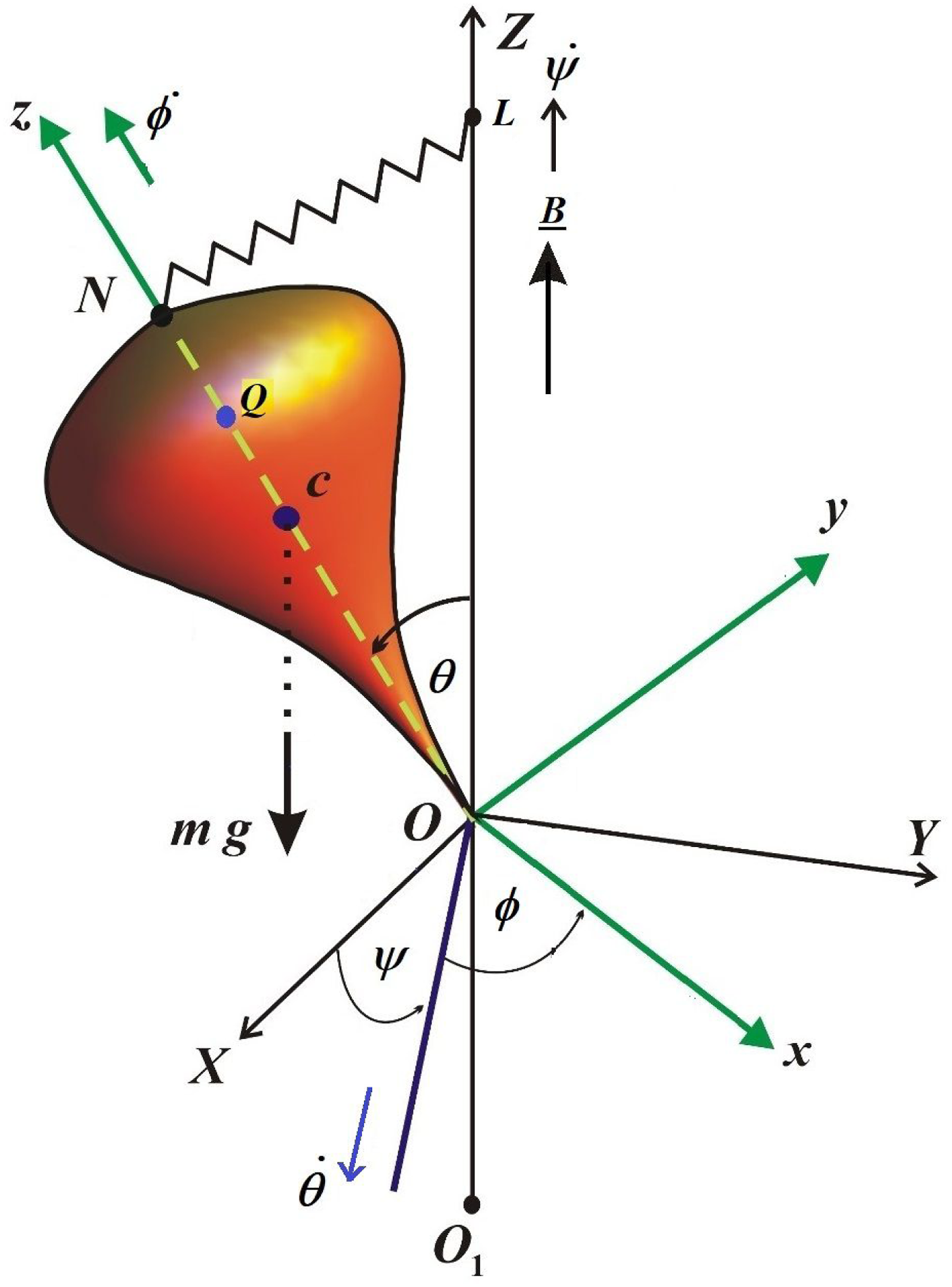
Let us consider the dynamically symmetric gyrostat of mass $m$ rotates about a fixed-point $O$ and is attached to a spring at some point $N$ with a fixed end at the point $L$ , (see Figure 1). Consider the two frames of coordinate systems: The fixed coordinate in space $OXYZ$ , and another moving one $Oxyz$ attached to the body. If the direction of the vector of the point $O_1$ to the point $O$ is $R$ . Take the mobile system axes in the direction of the principal inertia ones. Consider $\theta ,\psi ,$ and $\varphi$ represent the angles of Euler.

Figure 1.

Shows restricted dynamical symmetric gyrostat.

The acting forces of this body are the uniform gravitational force field, the Newtonian force resulting from the center $O_1$ , addition of the restoring torques, and perturbed ones $k_j\hspace{0.17em}\left(j=\mathrm{1,2}\right)$ and ${\tau }_i\hspace{0.17em}\left(i=\mathrm{1,2,3}\right)$ , respectively. If we consider $\nu$ being the spring stiffness, then the body suffers also from elastic force $F$ according to Hook’s low ²⁶

$F=\nu \left(s-s_0\right),$

(1)

where $s=s\left(\theta \right)=\mathit{LN}$ is the length of the spring with deformation $s_0$ . As the spring has hardened, the elastic force yields a restoring torque in the form

$k_1=mgl+\nu hz\left(1-s_0/\sqrt{h^2+z^2-2hz\cos \theta }\right),$

(2)

where $ON=z,Oc=l,OL=h,$ and $g$ is the gravity acceleration.

Let the body rotate around the symmetry $z$ -axis in an electromagnetic force field consisting of a charge $Q$ lying on that axis and a vertical magnetic field of strength $\underset{¯}{B}.$ Let $\underset{¯}{V}$ be the vector of the linear velocity for this rotation. The Lorentz force is obtained in the form $Q\left(\underset{¯}{V}\wedge \underset{¯}{B}\right)$ ²⁷ which gives a restoring torque on the form

$k_2=QB\hspace{0.17em}{l^{\prime }}^2\cos \theta \left|\left({\omega }_2,-{\omega }_1,0\right)\right|+N\left(I_3-I_1\right)\cos \theta ,$

(3)

where $l^{\prime }$ represents the distance between $O$ and $Q$ . We note that $k_2$ is dependent on the components ${\omega }_1$ and ${\omega }_2$ of the angular velocities, the inertia moments $I_1$ and $I_3$ , and on $\theta$ . Thus, from the above description and equations (2) and (3), we deduce that the gyrostat acted upon the gravity force, NFF, with the restoring torque $k=k_1+k_2$ .

Assuming the center of gravity and inertia moments are

$x_c=y_c=0,z_c=l,I_1=I_2\ne I_3.$

(4)

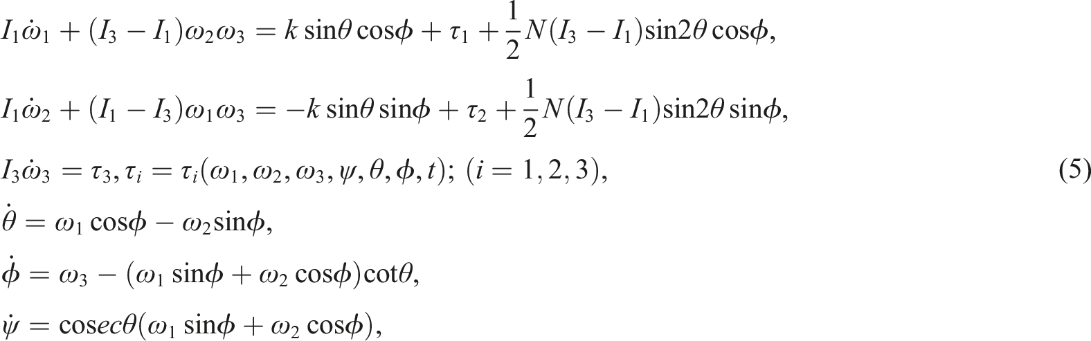
Supposing ${\tau }_i\hspace{0.17em}\left(i=\mathrm{1,2,3}\right)$ are the torques to the principal inertia axes for the body go through $O$ and $\lambda$ is the constant of the gravity. Let us assume the gyro rotates about a fixed-point $O$ , in the existence of a restoring torque vector and perturbation moments depending on a slow time $\tau =t/\epsilon$ . Where $\epsilon$ is a sufficiently large parameter distinguishes the magnitude of the perturbation and the time is $t$ . The differential equations for the moving system take the following forms^28,29

$\begin{array}{l}{I}_1{\dot{\omega }}_1+\left(I_3-I_1\right){\omega }_2{\omega }_3=k\hspace{0.17em}\sin \theta \hspace{0.17em}\cos \varphi +{\tau }_1+\frac{1}{2}N\left(I_3-I_1\right)\sin 2\theta \hspace{0.17em}\cos \varphi ,\\ I_1{\dot{\omega }}_2+\left(I_1-I_3\right){\omega }_1{\omega }_3=-k\hspace{0.17em}\sin \theta \hspace{0.17em}\sin \varphi +{\tau }_2+\frac{1}{2}N\left(I_3-I_1\right)\sin 2\theta \hspace{0.17em}\sin \varphi ,\\ I_3{\dot{\omega }}_3={\tau }_3,{\tau }_i={\tau }_i\left({\omega }_1,{\omega }_2,{\omega }_3,\psi ,\theta ,\varphi ,t\right);\hspace{0.17em}\left(i=\mathrm{1,2,3}\right),\\ \dot{\theta }={\omega }_1\hspace{0.17em}\cos \varphi -{\omega }_2\sin \varphi ,\\ \dot{\varphi }={\omega }_3-\left({\omega }_1\hspace{0.17em}\sin \varphi +{\omega }_2\hspace{0.17em}\cos \varphi \right)\cot \theta ,\\ \dot{\psi }=\cos ec\theta \left({\omega }_1\hspace{0.17em}\sin \varphi +{\omega }_2\hspace{0.17em}\cos \varphi \right),\end{array}$

(5)

where $N=3\lambda /R,\left({\omega }_1,{\omega }_2,{\omega }_3\right)$ are the angular velocity components around the axes $x,y,z$ , respectively; and $x_c,y_c,$ and $z_c$ are the center of mass coordinates of the body.

We assume that the perturbed torques are functions of a period $2\pi$ of $\theta ,\psi ,$ and $\varphi$ . Consider the maximum value of the varied restoring torque is

$k=mgl.$

(6)

We note that at ${\tau }_i=0,$ the equation (5) yield a similar case to Lagrange-Poisson. For ${\tau }_i=N=0,$ equation (5) give the uniform Lagrange-Poisson problem. Besides, equation (5), when $N=0,$ present the motion for the Lagrangian top influenced by perturbations of different natural origins, as well as the motion for a uniform solid body to its mass center when that object is subjected to a restoration torque due to the forces of aerodynamics and some perturbed torques.

Let us consider the initial conditions

${{\omega }_1}^2+{{\omega }_2}^2<<1,{\tau }_3\approx k>>\left|{\tau }_i\right|;\hspace{0.17em}\left(i=\mathrm{1,2}\right),$

(7)

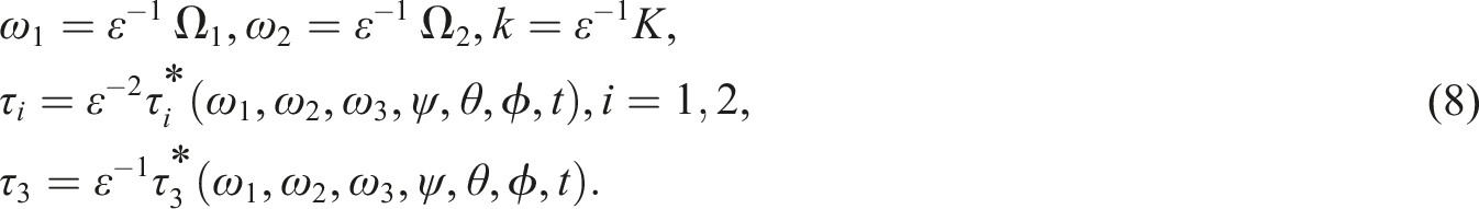
Conditions (7) show that the angular velocity components are taken as a smaller valued in direction of the axes $x$ and $y$ . The two projections ${\tau }_i$ for the perturbed torque vector of concern on the inertia main axes of the gyrostat are small compared with the restored torque $k$ , whereas ${\tau }_3$ is of the same size as that torque.

Assumptions (7) help us to present the large parameter $\epsilon$ and assignment

$\begin{array}{l}{\omega }_1={\epsilon }^{-1}\hspace{0.17em}{\mathrm{\Omega }}_1,{\omega }_2={\epsilon }^{-1}\hspace{0.17em}{\mathrm{\Omega }}_2,k={\epsilon }^{-1}K,\\ {\tau }_i={\epsilon }^{-2}{\tau }_i^{*}\left({\omega }_1,{\omega }_2,{\omega }_3,\psi ,\theta ,\varphi ,t\right),i=\mathrm{1,2},\\ {\tau }_3={\epsilon }^{-1}{\tau }_3^{*}\left({\omega }_1,{\omega }_2,{\omega }_3,\psi ,\theta ,\varphi ,t\right).\end{array}$

(8)

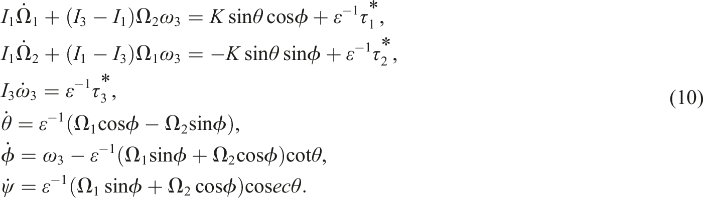
The newly introduced variables and constants ${\mathrm{\Omega }}_1,{\mathrm{\Omega }}_2,{\omega }_i,\psi ,\theta ,\varphi ,{\tau }_i^{*};\hspace{0.17em}\left(i=\mathrm{1,2,3}\right)$ and $K,I_1,I_3$ are supposed to bounded quantities from order unity when $\epsilon$ going to infinity. Under assumptions (7) and (8), the approximated solutions for system (5) when $\epsilon$ is sufficiently large will be considered. The averaging procedure is used through the large parameter to solve this problem on an interval of time with the order $\epsilon$ . We consider the following two cases, which are classified according to the restoring torque.

The variable restored torque

From assumptions (6) and (7), the restoring torque resultant $K$ is written as follows

$\begin{array}{l}K=mgl+\nu hz\left[1-s_0/\sqrt{h^2+z^2-2hz\cos \theta }\right]\\ +QB\hspace{0.17em}{l^{\prime }}^2\cos \theta \left({\omega }_2,-{\omega }_1,0\right)+N\left(I_3-I_1\right)\cos \theta .\end{array}$

(9)

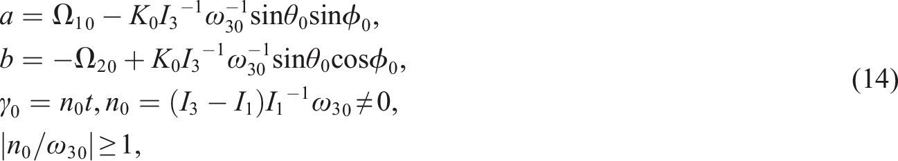
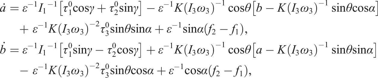
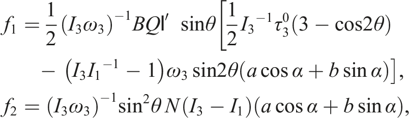
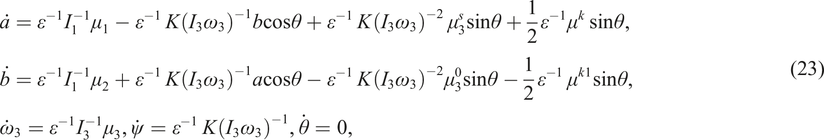
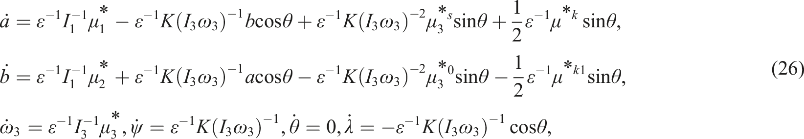
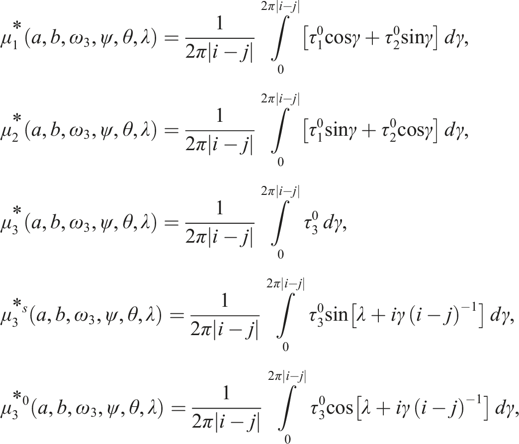
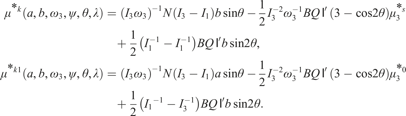
Using (5), (8), and (9) and cancelling $\epsilon$ on both sides of the first two equations, one gets

$\begin{array}{l}{I}_1{\dot{\mathrm{\Omega }}}_1+\left(I_3-I_1\right){\mathrm{\Omega }}_2{\omega }_3=K\hspace{0.17em}\sin \theta \hspace{0.17em}\cos \varphi +{\epsilon }^{-1}{\tau }_1^{*},\\ I_1{\dot{\mathrm{\Omega }}}_2+\left(I_1-I_3\right){\mathrm{\Omega }}_1{\omega }_3=-K\hspace{0.17em}\sin \theta \hspace{0.17em}\sin \varphi +{\epsilon }^{-1}{\tau }_2^{*},\\ I_3{\dot{\omega }}_3={\epsilon }^{-1}{\tau }_3^{*},\\ \dot{\theta }={\epsilon }^{-1}\left({\mathrm{\Omega }}_1\cos \varphi -{\mathrm{\Omega }}_2\sin \varphi \right),\\ \dot{\varphi }={\omega }_3-{\epsilon }^{-1}\left({\mathrm{\Omega }}_1\sin \varphi +{\mathrm{\Omega }}_2\cos \varphi \right)\cot \theta ,\\ \dot{\psi }={\epsilon }^{-1}\left({\mathrm{\Omega }}_1\hspace{0.17em}\sin \varphi +{\mathrm{\Omega }}_2\hspace{0.17em}\cos \varphi \right)\cos ec\theta .\end{array}$

(10)

Putting $\epsilon \to \infty$ in (10), we get

${\omega }_3={{\omega }_3}_0,\psi ={\psi }_0,\theta ={\theta }_0,\varphi ={\omega }_{30}t+{\varphi }_0,$

(11)

where ${{\omega }_3}_0,{\psi }_0,{\theta }_0,$ and ${\varphi }_0$ are initial values for the relevant quantities.

Making use of (11) into (10) for $\epsilon \to \infty ,$ yield

$\begin{array}{l}{\ddot{\mathrm{\Omega }}}_1+n_0^2{\mathrm{\Omega }}_1=K_0\left(n_0-{{\omega }_3}_0\right){I_1}^{-1}\sin {\theta }_0\sin \left({{\omega }_3}_{0}t+{\varphi }_0\right),\\ {\ddot{\mathrm{\Omega }}}_2+n_0^2{\mathrm{\Omega }}_2=K_0\left(n_0-{{\omega }_3}_0\right){I_1}^{-1}\sin {\theta }_0\cos \left({{\omega }_3}_{0}t+{\varphi }_0\right).\end{array}$

(12)

The solution of (12), gives

$\begin{array}{l}{\mathrm{\Omega }}_1=a\hspace{0.17em}\cos {\gamma }_0+b\hspace{0.17em}\sin {\gamma }_0+K_0{I_3}^{-1}{\omega }_{30}^{-1}\sin {\theta }_0\sin \left({{\omega }_3}_{0}t+{\varphi }_0\right),\\ {\mathrm{\Omega }}_2=a\hspace{0.17em}\sin {\gamma }_0-b\hspace{0.17em}\cos {\gamma }_0+K_0{I_3}^{-1}{\omega }_{30}^{-1}\sin {\theta }_0\cos \left({{\omega }_3}_{0}t+{\varphi }_0\right),\end{array}$

(13)

such that

$\begin{array}{l}a={{\mathrm{\Omega }}_1}_0-K_0{I_3}^{-1}{\omega }_{30}^{-1}\sin {\theta }_0\sin {\varphi }_0,\\ b=-{{\mathrm{\Omega }}_2}_0+K_0{I_3}^{-1}{\omega }_{30}^{-1}\sin {\theta }_0\cos {\varphi }_0,\\ {\gamma }_0=n_{0}t,n_0=\left(I_3-I_1\right){I_1}^{-1}{{\omega }_3}_0\ne 0,\\ \left|n_0/{{\omega }_3}_0\right|\ge 1,\end{array}$

(14)

where ${\mathrm{\Omega }}_{10}$ and ${\mathrm{\Omega }}_{20}$ are initial values for the corresponding quantities, and ${\gamma }_0$ is the phase of oscillation for the generated system when $\epsilon \to \infty .$

Equation (14) assumes that the body rotates with an initial slow spin around the $z$ -axis, which is minor, for the inertia ellipsoid $\left(I_1=I_2<I_3\right).$

Introducing the variable $\gamma$ in the form

$d\gamma =ndt,\gamma \left(0\right)=0.$

(15)

For $\epsilon \to \infty ,$ we get $\gamma ={\gamma }_0$ . Making use of (11) and (13) we obtain

$\begin{array}{l}{\mathrm{\Omega }}_1=a\hspace{0.17em}\cos \gamma +b\hspace{0.17em}\sin \gamma +K{I_3}^{-1}{{\omega }_3}^{-1}\sin \theta \sin \varphi ,\\ {\mathrm{\Omega }}_2=a\hspace{0.17em}\sin \gamma -b\hspace{0.17em}\cos \gamma +K{I_3}^{-1}{{\omega }_3}^{-1}\sin \theta \cos \varphi ,\end{array}\}$

(16)

For this case $a$ and $b$ take the form

$\begin{array}{l}a={\mathrm{\Omega }}_1\cos \gamma +{\mathrm{\Omega }}_2\sin \gamma -K{I_3}^{-1}{{\omega }_3}^{-1}\sin \theta \sin \left(\gamma +\varphi \right),\\ b={\mathrm{\Omega }}_1\sin \gamma -{\mathrm{\Omega }}_2\cos \gamma +K{I_3}^{-1}{{\omega }_3}^{-1}\sin \theta \cos \left(\gamma +\varphi \right).\end{array}$

(17)

Converting the variables ${\mathrm{\Omega }}_1,{\mathrm{\Omega }}_2,{\omega }_3,\psi ,\theta ,\varphi ,$ and $\gamma$ to the variables $a,b,{\omega }_3,\psi ,\theta ,\varphi ,\alpha ,$ and $\gamma$ when

$\alpha =\gamma +\varphi .$

(18)

After some processing, we get the following system

$\begin{array}{l}\dot{a}={\epsilon }^{-1}{I_1}^{-1}\left[{\tau }_1^0\cos \gamma +{\tau }_2^0\sin \gamma \right]-{\epsilon }^{-1}K{\left(I_3{\omega }_3\right)}^{-1}\cos \theta \left[b-K{\left(I_3{\omega }_3\right)}^{-1}\sin \theta \cos \alpha \right]\\ +{\epsilon }^{-1}K{\left(I_3{\omega }_3\right)}^{-2}{\tau }_3^0\sin \theta \sin \alpha +{\epsilon }^{-1}\sin \alpha \left(f_2-f_1\right),\\ \dot{b}={\epsilon }^{-1}{I_1}^{-1}\left[{\tau }_1^0\sin \gamma -{\tau }_2^0\cos \gamma \right]+{\epsilon }^{-1}K{\left(I_3{\omega }_3\right)}^{-1}\cos \theta \left[a-K{\left(I_3{\omega }_3\right)}^{-1}\sin \theta \sin \alpha \right]\\ -{\epsilon }^{-1}K{\left(I_3{\omega }_3\right)}^{-2}{\tau }_3^0\sin \theta \cos \alpha +{\epsilon }^{-1}\cos \alpha \left(f_2-f_1\right),\end{array}$

$\begin{array}{l}{\dot{\omega }}_3={\epsilon }^{-1}{I_3}^{-1}{\tau }_3^0,\\ \dot{\psi }={\epsilon }^{-1}\cos ec\theta \hspace{0.17em}\left(a\hspace{0.17em}\sin \alpha -b\hspace{0.17em}\cos \alpha \right)+{\epsilon }^{-1}K{\left(I_3{\omega }_3\right)}^{-1},\\ \dot{\theta }={\epsilon }^{-1}\left(a\hspace{0.17em}\cos \alpha +b\hspace{0.17em}\sin \alpha \right),\\ \dot{\alpha }=I_3{I_1}^{-1}{\omega }_3-{\epsilon }^{-1}\hspace{0.17em}\cot \theta \hspace{0.17em}\left(a\hspace{0.17em}\sin \alpha -b\hspace{0.17em}\cos \alpha \right)-\epsilon K{\left(I_3{\omega }_3\right)}^{-1}\cos \theta ,\\ d\gamma =\left(I_3{I_1}^{-1}-1\right){\omega }_{3}dt,\end{array}$

(19)

where

$\begin{array}{l}{f}_1=\frac{1}{2}{\left(I_3{\omega }_3\right)}^{-1}BQ{l}^{\prime }\sin \theta [\frac{1}{2}{I_3}^{-1}{\tau }_3^0\left(3-\cos 2\theta \right)\\ -\left(I_3{I_1}^{-1}-1\right){\omega }_3\hspace{0.17em}\sin 2\theta \left(a\hspace{0.17em}\cos \alpha +b\hspace{0.17em}\sin \alpha \right)],\\ f_2={\left(I_3{\omega }_3\right)}^{-1}{\sin }^2\theta \hspace{0.17em}N\left(I_3-I_1\right)\left(a\hspace{0.17em}\cos \alpha +b\hspace{0.17em}\sin \alpha \right),\end{array}$

and ${\tau }_i^0$ are obtained in terms of ${\tau }_i^{*}$ as follows

${\tau }_i^0\left(a,b,{\omega }_3,\psi ,\theta ,\alpha ,\gamma ,t\right)={\tau }_i^{*}\left({\mathrm{\Omega }}_1,{\mathrm{\Omega }}_2,{\omega }_3,\psi ,\theta ,\varphi ,t\right);\left(i=\mathrm{1,2,3}\right).$

(20)

Introducing the vector $X$ with slow variables components and rewriting system (19) as follows

$\begin{array}{l}\dot{X}={\epsilon }^{-1}X\left(x,\alpha ,\gamma ,t\right),\dot{\alpha }=I_3{I_1}^{-1}{\omega }_3+{\epsilon }^{-1}Y\left(x,\alpha \right),\\ d\gamma =\left(I_3{I_1}^{-1}-1\right){\omega }_3\hspace{0.17em}dt,x\left(0\right)=x_0,\alpha \left(0\right)={\alpha }_0,\gamma \left(0\right)=0,\end{array}$

(21)

where $X$ is a vector-valued function and $Y$ is a scalar one defined from the correspondence with the right-hand sides for (19).

The averaging for system (21) or (19) gives two cases named: the resonant and the non-resonant cases:

1. The case of resonance from the system (21) is given when

$I_3/I_1=i/j\le 2,$

(22)

where $i$ and $j$ are prime numbers.

2. The case of a non-resonance occurs when $I_3/I_1\ne i/j$ .

Considering the case of a non-resonant, the averaging of the system (19) to $\alpha$ and $\gamma$ (which are fast variables) gives

$\begin{array}{l}\dot{a}={\epsilon }^{-1}{I}_1^{-1}{\mu }_1-{\epsilon }^{-1}\hspace{0.17em}K{\left(I_3{\omega }_3\right)}^{-1}b\cos \theta +{\epsilon }^{-1}\hspace{0.17em}K{\left(I_3{\omega }_3\right)}^{-2}\hspace{0.17em}{\mu }_3^s\sin \theta +\frac{1}{2}{\epsilon }^{-1}{\mu }^k\hspace{0.17em}\sin \theta ,\\ \dot{b}={\epsilon }^{-1}{I}_1^{-1}{\mu }_2+{\epsilon }^{-1}\hspace{0.17em}K{\left(I_3{\omega }_3\right)}^{-1}a\cos \theta -{\epsilon }^{-1}\hspace{0.17em}K{\left(I_3{\omega }_3\right)}^{-2}{\mu }_3^0\sin \theta -\frac{1}{2}{\epsilon }^{-1}\hspace{0.17em}{\mu }^{k1}\sin \theta ,\\ {\dot{\omega }}_3={\epsilon }^{-1}{I}_3^{-1}{\mu }_3,\dot{\psi }={\epsilon }^{-1}\hspace{0.17em}K{\left(I_3{\omega }_3\right)}^{-1},\dot{\theta }=0,\end{array}$

(23)

such that

$\begin{array}{l}{\mu }_1=\frac{1}{4{\pi }^2}\underset{0}{\overset{2\pi }{{\displaystyle \int }}}\underset{0}{\overset{2\pi }{{\displaystyle \int }}}\left[{\tau }_1^0\cos \gamma +{\tau }_2^0\sin \gamma \right]\hspace{0.17em}d\alpha \hspace{0.17em}d\gamma ,\\ {\mu }_2=\frac{1}{4{\pi }^2}\underset{0}{\overset{2\pi }{{\displaystyle \int }}}\underset{0}{\overset{2\pi }{{\displaystyle \int }}}\left[{\tau }_1^0\sin \gamma -{\tau }_2^0\cos \gamma \right]\hspace{0.17em}d\alpha \hspace{0.17em}d\gamma ,\\ {\mu }_3=\frac{1}{4{\pi }^2}\underset{0}{\overset{2\pi }{{\displaystyle \int }}}\underset{0}{\overset{2\pi }{{\displaystyle \int }}}{\tau }_3^0\hspace{0.17em}d\alpha \hspace{0.17em}d\gamma ,\\ {\mu }_3^s=\frac{1}{4{\pi }^2}\underset{0}{\overset{2\pi }{{\displaystyle \int }}}\underset{0}{\overset{2\pi }{{\displaystyle \int }}}{\tau }_3^0\hspace{0.17em}\sin \alpha \hspace{0.17em}d\alpha \hspace{0.17em}d\gamma ,\\ {\mu }_3^0=\frac{1}{4{\pi }^2}\underset{0}{\overset{2\pi }{{\displaystyle \int }}}\underset{0}{\overset{2\pi }{{\displaystyle \int }}}{\tau }_3^0\hspace{0.17em}\cos \alpha \hspace{0.17em}d\alpha \hspace{0.17em}d\gamma ,\end{array}$

$\begin{array}{l}{\mu }^k={\left(I_3{\omega }_3\right)}^{-1}N\left(I_3-I_1\right)b\hspace{0.17em}\sin \theta -\frac{1}{2}{I}_3^{-2}{\omega }_3^{-1}BQ\hspace{0.17em}{l}^{\prime }\hspace{0.17em}\left(3-\cos 2\theta \right)\hspace{0.17em}{\mu }_3^s\\ +\frac{1}{2}\left(I_1^{-1}-I_3^{-1}\right)BQ\hspace{0.17em}{l}^{\prime }\hspace{0.17em}b\hspace{0.17em}\sin 2\theta ,\\ {\mu }^{k1}={\left(I_3{\omega }_3\right)}^{-1}N\left(I_3-I_1\right)a\hspace{0.17em}\sin \theta -\frac{1}{2}{I}_3^{-2}{\omega }_3^{-1}BQ\hspace{0.17em}{l}^{\prime }\hspace{0.17em}\left(3-\cos 2\theta \right)\hspace{0.17em}{\mu }_3^0\\ +\frac{1}{2}\left(I_1^{-1}-I_3^{-1}\right)BQ\hspace{0.17em}{l}^{\prime }\hspace{0.17em}a\hspace{0.17em}\sin 2\theta ,\end{array}$

The averaging of the system (23) is carried out in a suitable manner. ¹⁸ For the resonant case of the frequency motion, we introduce a slow variable

$\lambda =\alpha -i\gamma \hspace{0.17em}{\left(i-j\right)}^{-1},\left(i/j\right)\ne 1,\left(i/j\right)\le 2\hspace{0.17em};i,j>0.$

(24)

The following standard rotating phase system of the system (21) is obtained

$\begin{array}{l}\dot{X}={\epsilon }^{-1}X\hspace{0.17em}{(x,i\gamma \hspace{0.17em}(i-j)}^{-1}+\lambda ,\gamma ),\\ \dot{\lambda }={\epsilon }^{-1}\hspace{0.17em}Y{(x,i\gamma \hspace{0.17em}(i-j)}^{-1}+\lambda ),\\ \dot{\gamma }=\left(I_3-I_1\right)\hspace{0.17em}{I_1}^{-1}{\omega }_3.\end{array}$

(25)

Averaging the system (25) to the period $2\left|i-j\right|\pi$ in $\gamma$ , we get

$\begin{array}{l}\dot{a}={\epsilon }^{-1}{I}_1^{-1}{\mu }_1^{*}-{\epsilon }^{-1}K{\left(I_3{\omega }_3\right)}^{-1}b\cos \theta +{\epsilon }^{-1}K{\left(I_3{\omega }_3\right)}^{-2}{\mu }_3^{*s}\sin \theta +\frac{1}{2}{\epsilon }^{-1}{\mu }^{*k}\hspace{0.17em}\sin \theta ,\\ \dot{b}={\epsilon }^{-1}{I}_1^{-1}{\mu }_2^{*}+{\epsilon }^{-1}K{\left(I_3{\omega }_3\right)}^{-1}a\cos \theta -{\epsilon }^{-1}K{\left(I_3{\omega }_3\right)}^{-2}{\mu }_3^{*0}\sin \theta -\frac{1}{2}{\epsilon }^{-1}{\mu }^{*k1}\sin \theta ,\\ {\dot{\omega }}_3={\epsilon }^{-1}{I}_3^{-1}{\mu }_3^{*},\dot{\psi }={\epsilon }^{-1}K{\left(I_3{\omega }_3\right)}^{-1},\dot{\theta }=0,\dot{\lambda }=-{\epsilon }^{-1}K{\left(I_3{\omega }_3\right)}^{-1}\cos \theta ,\end{array}$

(26)

here

$\begin{array}{l}{\mu }_1^{*}\left(a,b,{\omega }_3,\psi ,\theta ,\lambda \right)=\frac{1}{2\pi \left|i-j\right|}\underset{0}{\overset{2\pi \left|i-j\right|}{{\displaystyle \int }}}\left[{\tau }_1^0\cos \gamma +{\tau }_2^0\sin \gamma \right]\hspace{0.17em}d\gamma ,\\ {\mu }_2^{*}\left(a,b,{\omega }_3,\psi ,\theta ,\lambda \right)=\frac{1}{2\pi \left|i-j\right|}\underset{0}{\overset{2\pi \left|i-j\right|}{{\displaystyle \int }}}\left[{\tau }_1^0\sin \gamma +{\tau }_2^0\cos \gamma \right]\hspace{0.17em}d\gamma ,\\ {\mu }_3^{*}\left(a,b,{\omega }_3,\psi ,\theta ,\lambda \right)=\frac{1}{2\pi \left|i-j\right|}\underset{0}{\overset{2\pi \left|i-j\right|}{{\displaystyle \int }}}{\tau }_3^0\hspace{0.17em}d\gamma ,\\ {\mu }_3^{*s}\left(a,b,{\omega }_3,\psi ,\theta ,\lambda \right)=\frac{1}{2\pi \left|i-j\right|}\underset{0}{\overset{2\pi \left|i-j\right|}{{\displaystyle \int }}}{\tau }_3^0\sin \left[\lambda +i\gamma \hspace{0.17em}{\left(i-j\right)}^{-1}\right]\hspace{0.17em}d\gamma ,\\ {\mu }_3^{*0}\left(a,b,{\omega }_3,\psi ,\theta ,\lambda \right)=\frac{1}{2\pi \left|i-j\right|}\underset{0}{\overset{2\pi \left|i-j\right|}{{\displaystyle \int }}}{\tau }_3^0\cos \left[\lambda +i\gamma \hspace{0.17em}{\left(i-j\right)}^{-1}\right]\hspace{0.17em}d\gamma ,\end{array}$

$\begin{array}{l}{\mu }^{*k}\left(a,b,{\omega }_3,\psi ,\theta ,\lambda \right)={\left(I_3{\omega }_3\right)}^{-1}N\left(I_3-I_1\right)b\hspace{0.17em}\sin \theta -\frac{1}{2}{I}_3^{-2}{\omega }_3^{-1}BQ\hspace{0.17em}{l}^{\prime }\hspace{0.17em}\left(3-\cos 2\theta \right){\mu }_3^{*s}\\ +\frac{1}{2}\left(I_1^{-1}-I_1^{-1}\right)BQ\hspace{0.17em}{l}^{\prime }b\hspace{0.17em}\sin 2\theta ,\\ {\mu }^{*k1}\left(a,b,{\omega }_3,\psi ,\theta ,\lambda \right)={\left(I_3{\omega }_3\right)}^{-1}N\left(I_3-I_1\right)a\hspace{0.17em}\sin \theta -\frac{1}{2}{I}_3^{-2}{\omega }_3^{-1}BQ\hspace{0.17em}{l}^{\prime }\hspace{0.17em}\left(3-\cos 2\theta \right){\mu }_3^{*0}\\ +\frac{1}{2}\left({I_1}^{-1}-I_3^{-1}\right)BQ\hspace{0.17em}{l}^{\prime }b\hspace{0.17em}\sin 2\theta .\end{array}$

Thus, the motion of the gyrostat in this case is determined.

The perturbed torques as a sum of linear dissipative

Consider the linear dissipative perturbed torques like the Lagrange case as follows

$\begin{array}{l}{\tau }_1=-{\epsilon }^{-1}{J}_1{\omega }_1,{\tau }_2=-{\epsilon }^{-1}{J}_1{\omega }_2,\\ {\tau }_3=-{\epsilon }^{-1}{J}_3{\omega }_3+{\epsilon }^{-1}{\tau }_3^{*};J_1,J_3>0,\end{array}$

(27)

where $J_3$ and $J_1$ are constants that depend on the gyro characteristics. Making use of (8) and (27) we get

$\begin{array}{l}{\tau }_1=-{\epsilon }^{-2}{J}_1{\mathrm{\Omega }}_1,{\tau }_2=-{\epsilon }^{-2}{J}_1{\mathrm{\Omega }}_2,\\ {\tau }_3=-{\epsilon }^{-1}{J}_3{\omega }_3+{\epsilon }^{-1}{\tau }_3^{*};J_1,J_3>0.\end{array}$

(28)

For the non-resonance case of fundamental oscillations, we average system (23) to be

$\begin{array}{l}\dot{a}={\epsilon }^{-1}a{J}_1{I}_1^{-1}-{\epsilon }^{-1}\hspace{0.17em}b{\left(I_3{\omega }_3\right)}^{-1}K\cos \theta \\ -\frac{1}{2}{\epsilon }^{-1}b\hspace{0.17em}\sin \theta \hspace{0.17em}\left[{\left(I_3{\omega }_3\right)}^{-1}N\hspace{0.17em}\sin \theta \left(I_1-I_3\right)+\frac{1}{2}BQ\hspace{0.17em}{l}^{\prime }\sin 2\theta \left(I_3^{-1}-I_1^{-1}\right)\right],\\ \dot{b}=-{\epsilon }^{-1}b\hspace{0.17em}{J}_1{I}_1^{-1}+{\epsilon }^{-1}a{\left(I_3{\omega }_3\right)}^{-1}K\cos \theta \\ +\frac{1}{2}{\epsilon }^{-1}a\hspace{0.17em}\sin \theta \hspace{0.17em}\left[{\left(I_3{\omega }_3\right)}^{-1}N\hspace{0.17em}\sin \theta \left(I_1-I_3\right)+\frac{1}{2}BQ\hspace{0.17em}{l}^{\prime }\sin 2\theta \left(I_3^{-1}-I_1^{-1}\right)\right],\\ {\dot{\omega }}_3=-{\epsilon }^{-1}{I}_3^{-1}\left(J_3{\omega }_3-{\tau }_3^{*}\right),\dot{\psi }={\epsilon }^{-1}K{\left(I_3{\omega }_3\right)}^{-1},\dot{\theta }=0.\end{array}$

(29)

From (29), we get

${\omega }_3=\left({{\omega }_3}_0-{\tau }_3^{*}{J}_3^{-1}\right)\exp \left(-{\epsilon }^{-1}{I}_3^{-1}{J}_{3}t\right)+{\tau }_3^{*}{J}_3^{-1}.$

(30)

Substituting (30) into (29), we get

$\psi ={\psi }_0+K{{\tau }_3^{*}}^{-1}\ln \left|\frac{1+\left({{\omega }_3}_o{J}_3{\tau }_3^{*-1}-1\right)\exp \left(-{\epsilon }^{-1}{I}_3^{-1}{J}_{3}t\right)}{{{\omega }_3}_0{J}_3{\tau }_3^{*-1}}\right|+{\epsilon }^{-1}K{J}_3{\left(I_3{\tau }_3^{*}\right)}^{-1}t.$

(31)

From (29), we note that the nutation angle $\theta$ is still constant, that is,

$\theta ={\theta }_0.$

(32)

Considering (29), (30), and (32), we get

$\begin{array}{l}a=-b{I}_1{J}_3{K}_1{\left(I_3{J}_1{\tau }_3^{*}\right)}^{-1}-\frac{1}{4}BQ\hspace{0.17em}{l}^{\prime }\hspace{0.17em}b{J}_1^{-1}\left(I_1{I}_3^{-1}-1\right)\sin {\theta }_o\hspace{0.17em}\sin 2{\theta }_o\\ -{\epsilon }^{-2}b{J}_3{I}_3^{-1}{\tau }_3^{*-1}{K}_1\left(J_1{I}_1^{-1}+I_3^{-1}{\tau }_3^{*}{{\omega }_3}_0^{-1}\right)+{\chi }_1\hspace{0.17em}\exp \left(-{\epsilon }^{-1}{J}_1{I}_1^{-1}t\right),\\ b=-\frac{1}{4}{J}_1^{-1}BQ\hspace{0.17em}{l}^{\prime }\left(1-I_1{I}_3^{-1}\right)\sin 2{\theta }_o\hspace{0.17em}\sin {\theta }_o+I_1{{\omega }_3}_0^{-1}a{I}_3^{-1}{K}_1\\ -{\epsilon }^{-2}a{{\omega }_3}_0^2{I}_3^{-2}\left({{\omega }_3}_0{J}_3-{\tau }_3^{*}\right)K_1+{\chi }_2\hspace{0.17em}\exp \left(-{\epsilon }^{-1}{J}_1{I}_1^{-1}t\right),\end{array}$

(33)

where

$\begin{array}{l}{K}_1=\left[K+N\left(I_1-I_3\right)\sin {\theta }_0\right]\hspace{0.17em}\cos {\theta }_0,\\ {\chi }_1={\mathrm{\Omega }}_{10}-K_0{I}_3^{-1}{\omega }_{30}^{-1}\sin {\theta }_0\hspace{0.17em}\sin {\varphi }_0-{\left(J_1{I}_3\right)}^{-1}\left({{\mathrm{\Omega }}_2}_0-K_0{I}_3^{-1}{\omega }_{30}^{-1}\sin {\theta }_0\hspace{0.17em}\cos {\varphi }_0\right)\\ \times \left[A{J}_3{K}_1{\tau }_3^{*-1}+\frac{1}{4}BQ\hspace{0.17em}{l}^{\prime }\left(I_1-I_3\right)\sin 2{\theta }_0\hspace{0.17em}\sin {\theta }_0\right],\\ {\chi }_2=-{{\mathrm{\Omega }}_2}_0+K_0{\left(I_3{{\omega }_3}_0\right)}^{-1}\sin {\theta }_0\hspace{0.17em}\cos {\varphi }_o-{\left(J_1{I}_3\right)}^{-1}\left({{\mathrm{\Omega }}_1}_0-K_0{I}_3^{-1}{\omega }_{30}^{-1}\sin {\theta }_0\hspace{0.17em}\sin {\varphi }_0\right)\\ \times \left[\frac{1}{4}BQ\hspace{0.17em}{l}^{\prime }\left(I_1-I_3\right)\sin 2{\theta }_0\hspace{0.17em}\sin {\theta }_0+I_1{\omega }_{30}^{-1}{K}_1\right].\end{array}$

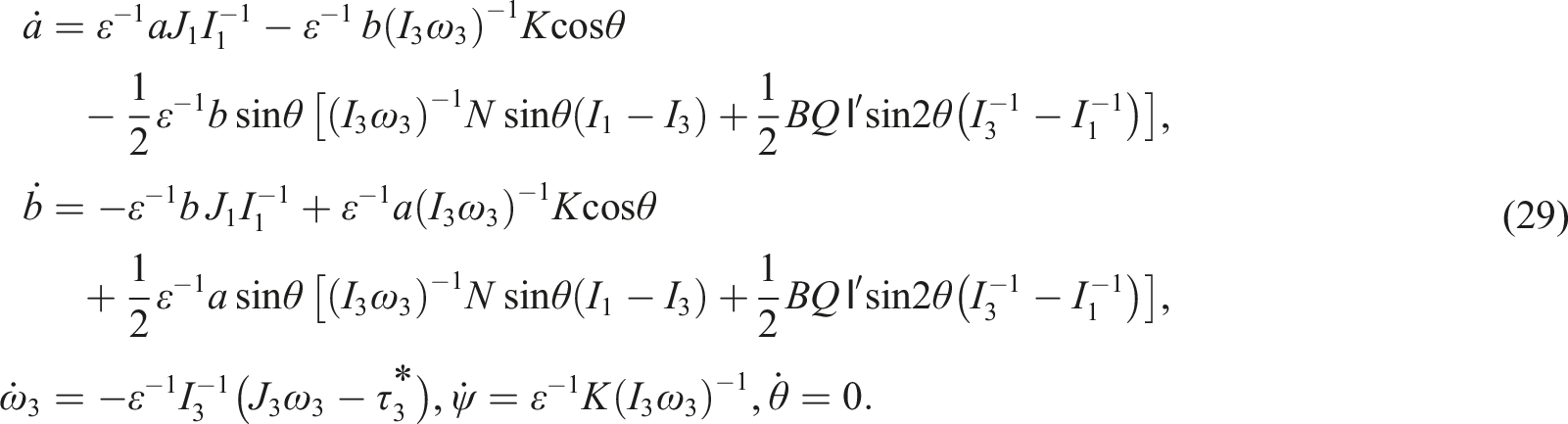
Therefore, we have obtained the first approximate solution for the considered system with the slow variables and dissipative torque case (27). If the resonance condition (22) is investigated, then the averaging must be obtained in analogously to the scheme (26). For this case, the integral relations ${{\mu }_i}^{*}$ in (26) coincide with the corresponding formulas ${\mu }_i$ for (23). Thus, the resonance does not accumulate until the resulting solution is suitable to describe the motion of any ratio $I_3\ne I_1.$

Numerical considerations

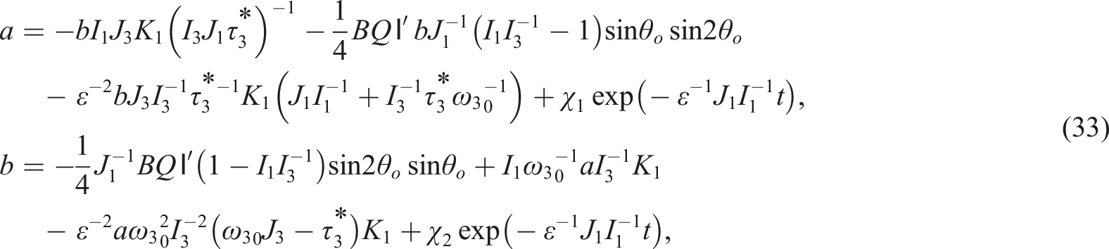
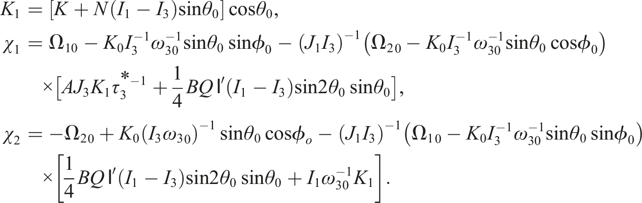
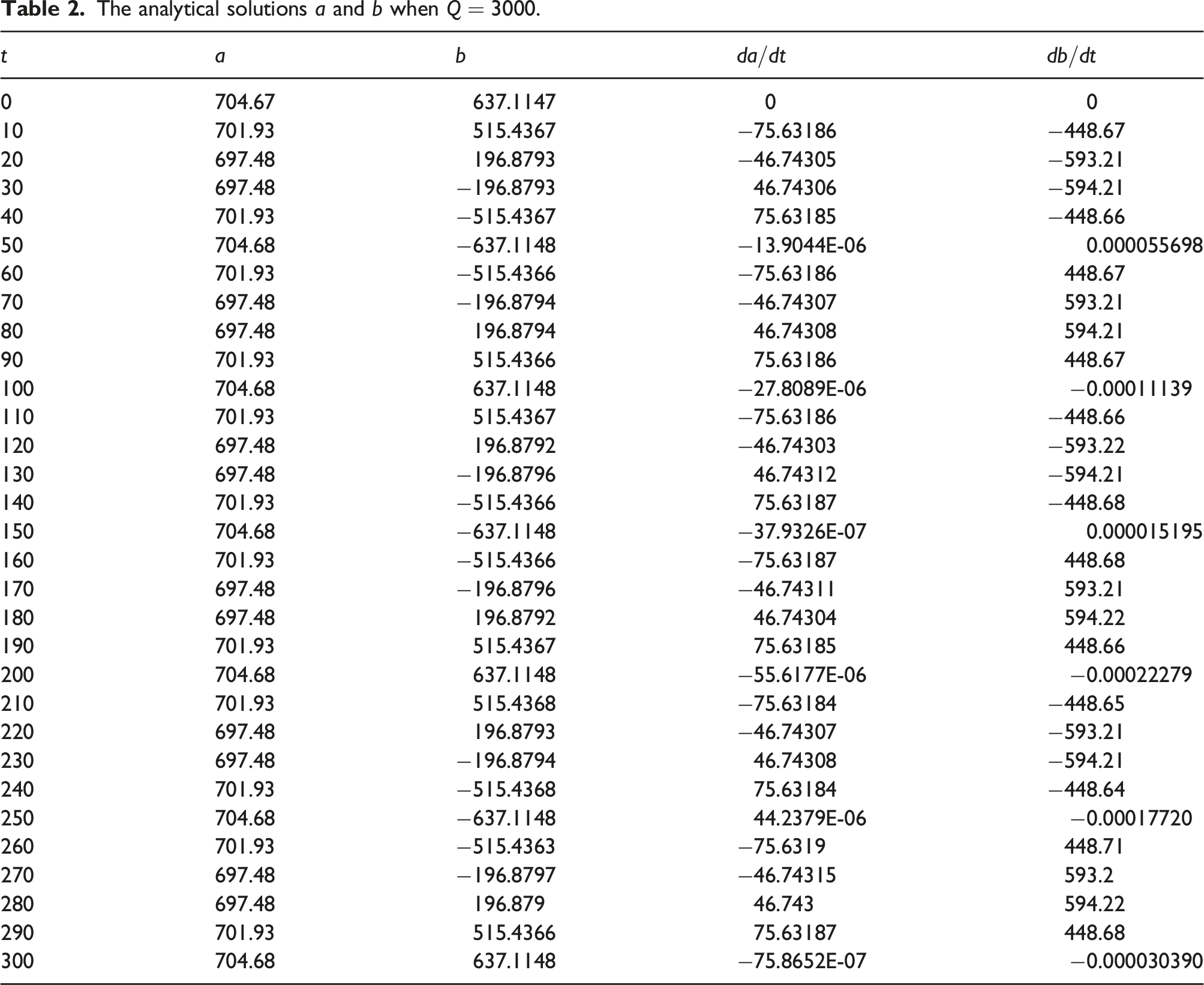
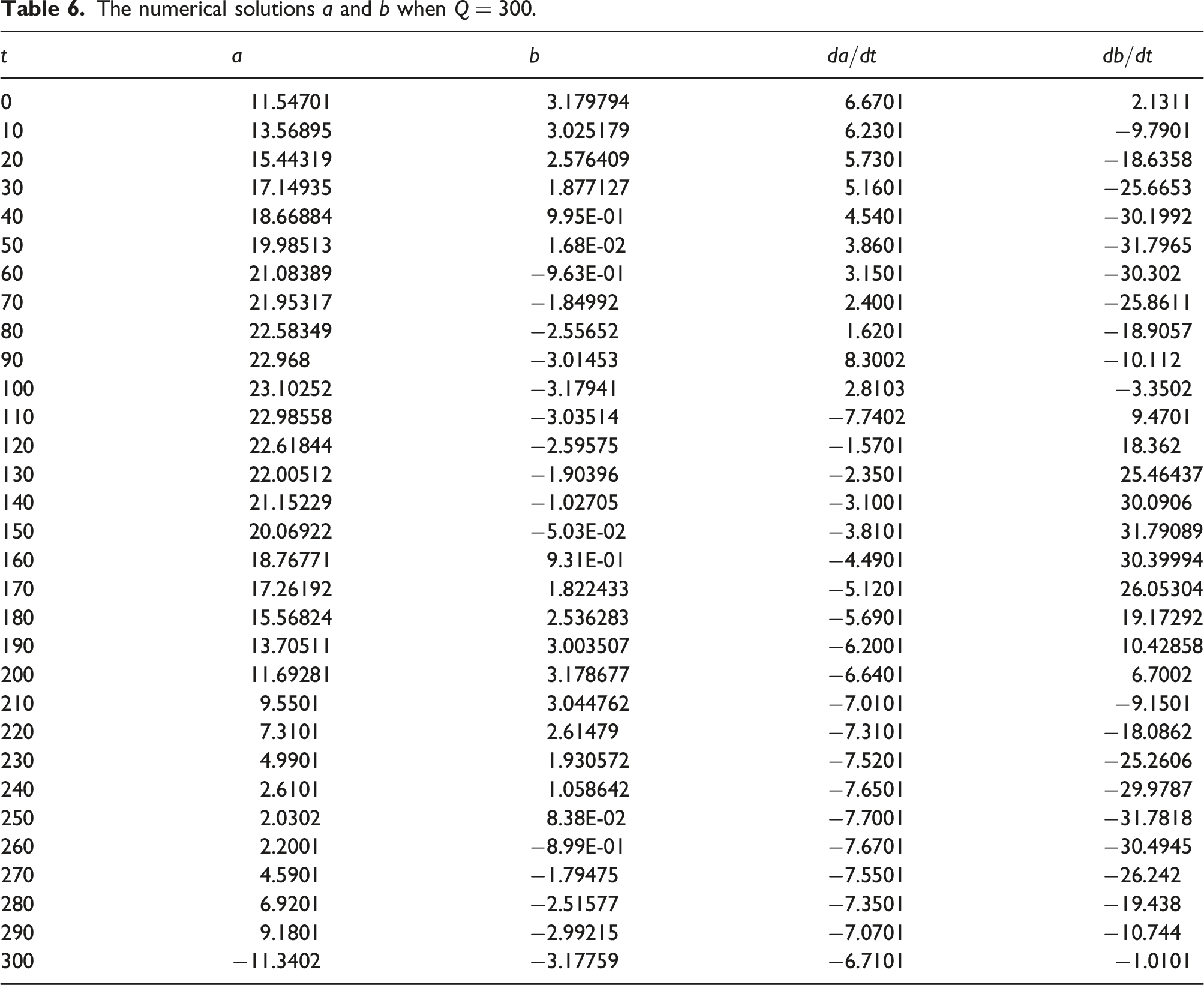
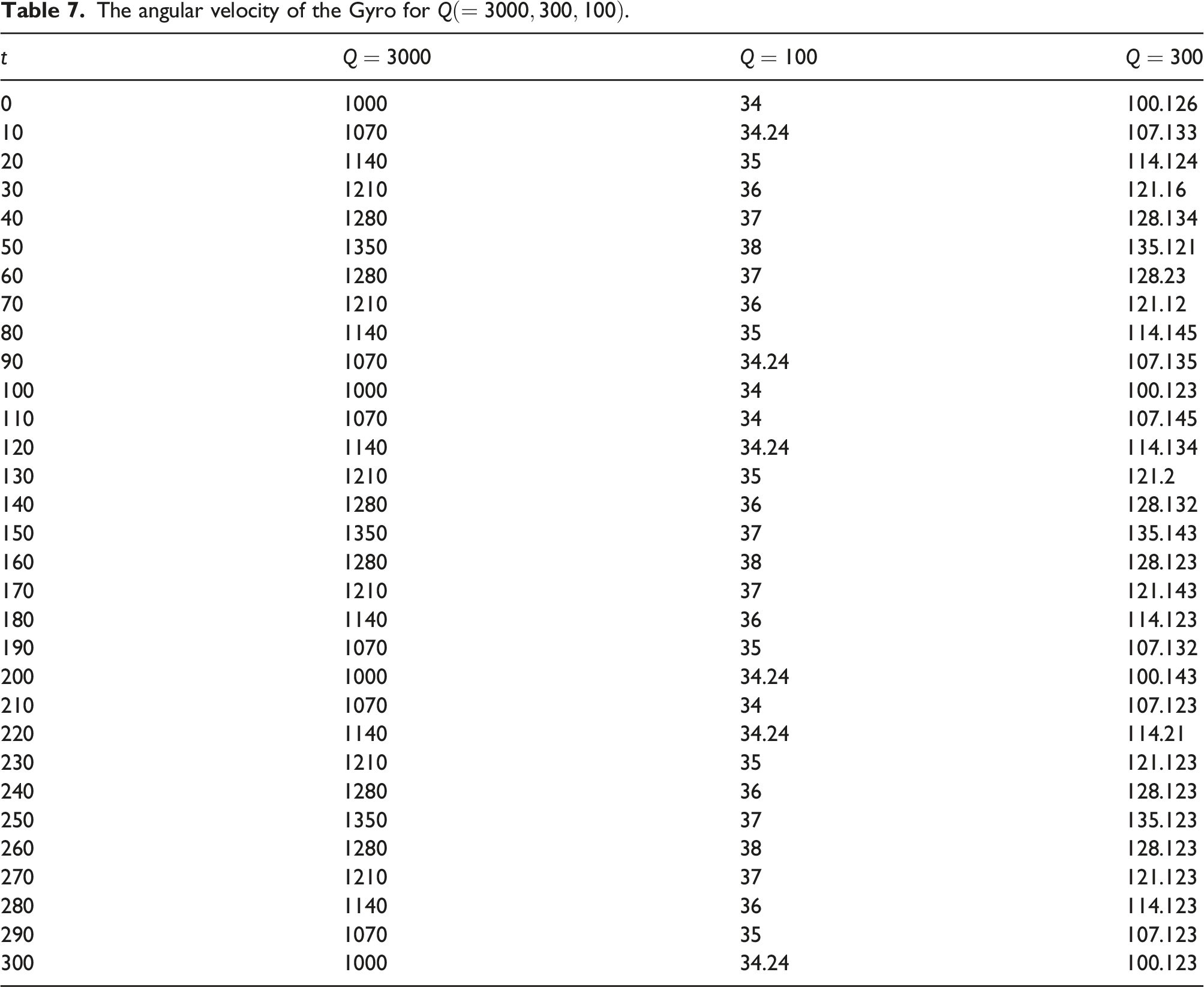
This section illustrates a qualitative analysis of the obtained results, explanations, and many diagrams. The analytical solutions of system (33) are drawn by computer programs for obtaining the geometric behavior of our solutions, which are represented when the point charge $Q\left(=\mathrm{100,3000,300}\right)$ Gausses and given by Tables 1–3. From the other side, system (23) can be solved numerically using the fourth-order Runge-Kutta of the method through other programs to obtain the numerical solutions for this system, taking into consideration the same values of initial conditions and point charge. The results are given in Tables 4–6. From these tables, we note that, when the point charge increases from $300$ to $3000$ Gausses, the amplitude of the solutions increase and vice versa. In the other direction, when the point charge decreases from $300$ to $100$ Gausses, the amplitude of the solution $a$ decreases while the amplitude of the solution $b$ increases and vice versa. The angular velocity $\omega ={\left({{\omega }_1}^2+{{\omega }_2}^2+{{\omega }_3}^2\right)}^{1/2}$ of the gyrostat increases when the point charge $Q$ increases and vice versa, see Table 7.

Table 1.

The analytical solutions $a$ and $b$ when $Q=100$ .

$t$	$a$	$b$	$da/dt$	$db/dt$
0	1.88116E-10	10	0	0
10	1.52189E-10	8.09017	−1.10572E-10	−5.87785
20	5.81312E-11	3.09017	−1.78909E-10	−9.51057
30	−5.81312E-11	−3.09017	−1.78909E-10	−9.51056
40	−1.5219E-10	−8.09017	−1.10572E-10	−5.87785
50	−1.88117E-10	−10	−2.84048E-17	−1.50996E-06
60	−1.52189E-10	−8.09017	1.10572E-10	5.87785
70	−5.81312E-11	−3.09017	1.78909E-10	9.51056
80	5.81312E-11	3.09017	1.78909E-10	9.51056
90	1.5219E-10	8.09017	1.10572E-10	5.87785
100	1.88117E-10	10	5.68096E-17	3.01992E-06
110	1.52189E-10	8.09017	−1.10572E-10	−5.87785
120	5.81312E-11	3.09017	−1.78909E-10	−9.51057
130	−5.81313E-11	−3.09017	−1.78909E-10	−9.51056
140	−1.52189E-10	−8.09017	−1.10572E-10	−5.87785
150	−1.88117E-10	−10	4.48654E-18	2.38498E-07
160	−1.52189E-10	−8.09017	1.10572E-10	5.87785
170	−5.81311E-11	−3.09016	1.78909E-10	9.51057
180	5.81314E-11	3.09018	1.78909E-10	9.51056
190	1.5219E-10	8.09017	1.10572E-10	5.87785
200	1.88117E-10	10	1.13619E-16	6.03983E-06
210	1.5219E-10	8.09017	−1.10572E-10	−5.87785
220	5.81312E-11	3.09017	−1.78909E-10	−9.51056
230	−5.81312E-11	−3.09017	−1.78909E-10	−9.51056
240	−1.5219E-10	−8.09017	−1.10572E-10	−5.87785
250	−1.88117E-10	−10	1.27079E-16	6.75532E-06
260	−1.52189E-10	−8.09016	1.10572E-10	5.87786
270	−5.81313E-11	−3.09018	1.78909E-10	9.51056
280	5.81311E-11	3.09017	1.78909E-10	9.51057
290	1.52189E-10	8.09017	1.10572E-10	5.87785
300	1.88117E-10	10	−8.97307E-18	−4.76995E-07

Table 2.

The analytical solutions $a$ and $b$ when $Q=3000$ .

$t$	$a$	$b$	$da/dt$	$db/dt$
0	704.67	637.1147	0	0
10	701.93	515.4367	−75.63186	−448.67
20	697.48	196.8793	−46.74305	−593.21
30	697.48	−196.8793	46.74306	−594.21
40	701.93	−515.4367	75.63185	−448.66
50	704.68	−637.1148	−13.9044E-06	0.000055698
60	701.93	−515.4366	−75.63186	448.67
70	697.48	−196.8794	−46.74307	593.21
80	697.48	196.8794	46.74308	594.21
90	701.93	515.4366	75.63186	448.67
100	704.68	637.1148	−27.8089E-06	−0.00011139
110	701.93	515.4367	−75.63186	−448.66
120	697.48	196.8792	−46.74303	−593.22
130	697.48	−196.8796	46.74312	−594.21
140	701.93	−515.4366	75.63187	−448.68
150	704.68	−637.1148	−37.9326E-07	0.000015195
160	701.93	−515.4366	−75.63187	448.68
170	697.48	−196.8796	−46.74311	593.21
180	697.48	196.8792	46.74304	594.22
190	701.93	515.4367	75.63185	448.66
200	704.68	637.1148	−55.6177E-06	−0.00022279
210	701.93	515.4368	−75.63184	−448.65
220	697.48	196.8793	−46.74307	−593.21
230	697.48	−196.8794	46.74308	−594.21
240	701.93	−515.4368	75.63184	−448.64
250	704.68	−637.1148	44.2379E-06	−0.00017720
260	701.93	−515.4363	−75.6319	448.71
270	697.48	−196.8797	−46.74315	593.2
280	697.48	196.879	46.743	594.22
290	701.93	515.4366	75.63187	448.68
300	704.68	637.1148	−75.8652E-07	−0.000030390

Table 3.

The analytical solutions $a$ and $b$ when $Q=300$ .

$t$	$a$	$b$	$da/dt$	$db/dt$
0	11.54701	3.179794	6.6701	2.1311
10	13.56894	3.025179	6.2302	−9.7902
20	15.44319	2.576409	5.7301	−18.6358
30	17.14934	1.877127	5.1601	−25.6653
40	18.66884	9.95E-01	4.5402	−30.1992
50	19.98513	1.68E-02	3.8601	−31.7964
60	21.08389	−9.63E-01	3.1501	−30.302
70	21.95317	−1.84992	2.4002	−25.8611
80	22.58349	−2.55652	1.6201	−18.9057
90	22.968	−3.01453	8.3002	−10.112
100	23.10252	−3.17941	2.8103	−3.3502
110	22.98558	−3.03514	−7.7402	9.4701
120	22.61844	−2.59574	−1.5701	18.362
130	22.00512	−1.90396	−2.3501	25.46437
140	21.15229	−1.02704	−3.1002	30.0906
150	20.06922	−5.03E-02	−3.8101	31.79089
160	18.76771	9.31E-01	−4.4901	30.39994
170	17.26192	1.822433	−5.1202	26.05304
180	15.56824	2.536283	−5.6901	19.17292
190	13.70511	3.003507	−6.2001	10.42858
200	11.69281	3.178677	−6.6402	6.7002
210	9.5501	3.044762	−7.0101	−9.1501
220	7.3101	2.61479	−7.3101	−18.0862
230	4.9901	1.930572	−7.5202	−25.2606
240	2.6101	1.058642	−7.6501	−29.9787
250	2.0302	8.38E-02	−7.7001	−31.7818
260	2.2001	−8.99E-01	−7.6702	−30.4944
270	4.5901	−1.79474	−7.5501	−26.242
280	6.9201	−2.51577	−7.3501	−19.438
290	9.1801	−2.99214	−7.0702	−10.744
300	−11.3402	−3.17759	−6.7101	−1.0101

Table 4.

The numerical solutions $a$ and $b$ when $Q=100$ .

$t$	$a$	$b$	$da/dt$	$db/dt$
0	1.88116E-10	10	0	0
10	1.52188E-10	8.09017	−1.10571E-10	−5.87784
20	5.81311E-11	3.09016	−1.78909E-10	−9.51057
30	−5.81311E-11	−3.09017	−1.78908E-10	−9.51056
40	−1.5218E-10	−8.09017	−1.10571E-10	−5.87784
50	−1.88116E-10	−10	−2.84048E-17	−1.50996E-06
60	−1.52188E-10	−8.09016	1.10571E-10	5.87784
70	−5.81311E-11	−3.09016	1.78909E-10	9.51056
80	5.81311E-11	3.090176	1.78909E-10	9.51056
90	1.5218E-10	8.09016	1.10571E-10	5.87784
100	1.88116E-10	10	5.68096E-17	3.01992E-06
110	1.52188E-10	8.09017	−1.10571E-10	−5.87784
120	5.81311E-11	3.09016	−1.78909E-10	−9.51057
130	−5.81312E-11	−3.09017	−1.78909E-10	−9.51056
140	−1.52188E-10	−8.09016	−1.10571E-10	−5.87784
150	−1.88116E-10	−10	4.48654E-18	2.38498E-07
160	−1.52188E-10	−8.09017	1.10571E-10	5.87784
170	−5.81310E-11	−3.09016	1.78908E-10	9.51057
180	5.81313E-11	3.09018	1.78908E-10	9.51056
190	1.5218E-10	8.09017	1.10572E-10	5.87784
200	1.88116E-10	10	1.13618E-16	6.03983E-06
210	1.5218E-10	8.09016	−1.10571E-10	−5.87784
220	5.81311E-11	3.09016	−1.78909E-10	−9.51056
230	−5.81311E-11	−3.09016	−1.78909E-10	−9.51056
240	−1.5218E-10	−8.09016	−1.10571E-10	−5.87784
250	−1.88116E-10	−10	1.27079E-16	6.75532E-06
260	−1.52188E-10	−8.09015	1.10572E-10	5.87786
270	−5.81312E-11	−3.09017	1.78908E-10	9.51056
280	5.81310E-11	3.09016	1.78909E-10	9.51057
290	1.52188E-10	8.09016	1.10571E-10	5.87784
300	1.88116E-10	10	−8.97307E-18	−4.76995E-07

Table 5.

The numerical solutions $a$ and $b$ when $Q=3000$ .

$t$	$a$	$b$	$da/dt$	$db/dt$
0	704.67	637.1147	0	0
10	701.93	515.4367	−75.63185	−448.66
20	697.48	196.8793	−46.74305	−593.21
30	697.48	−196.8793	46.74306	−594.21
40	701.93	−515.4367	75.63184	−448.66
50	704.67	−637.1147	−13.9044E-06	0.000055698
60	701.93	−515.4366	−75.63185	448.66
70	697.48	−196.8794	−46.74307	593.21
80	697.48	196.8794	46.74308	594.21
90	701.93	515.4366	75.63185	448.66
100	704.67	637.1147	−27.8089E-06	−0.00011139
110	701.93	515.4367	−75.63186	−448.67
120	697.48	196.8792	−46.74305	−593.22
130	697.48	−196.8796	46.74312	−594.21
140	701.93	−515.4366	75.63187	−448.67
150	704.67	−637.1147	−37.9326E-07	0.000015195
160	701.93	−515.4366	−75.63186	448.68
170	697.48	−196.8796	−46.74311	593.21
180	697.48	196.8792	46.74304	594.22
190	701.93	515.4367	75.63185	448.67
200	704.67	637.1147	−55.6177E-06	−0.00022279
210	701.93	515.4368	−75.63184	−448.65
220	697.48	196.8793	−46.74307	−593.21
230	697.48	−196.8794	46.74308	−594.21
240	701.93	−515.4368	75.63184	−448.63
250	704.67	−637.1147	44.2379E-06	−0.00017720
260	701.93	−515.4363	−75.6319	448.71
270	697.48	−196.8797	−46.74315	593.2
280	697.48	196.879	46.743	594.21
290	701.93	515.4366	75.63186	448.68
300	704.67	637.1147	−75.8652E-07	−0.000030380

Table 6.

The numerical solutions $a$ and $b$ when $Q=300$ .

t	a	b	$da/dt$	$db/dt$
0	11.54701	3.179794	6.6701	2.1311
10	13.56895	3.025179	6.2301	−9.7901
20	15.44319	2.576409	5.7301	−18.6358
30	17.14935	1.877127	5.1601	−25.6653
40	18.66884	9.95E-01	4.5401	−30.1992
50	19.98513	1.68E-02	3.8601	−31.7965
60	21.08389	−9.63E-01	3.1501	−30.302
70	21.95317	−1.84992	2.4001	−25.8611
80	22.58349	−2.55652	1.6201	−18.9057
90	22.968	−3.01453	8.3002	−10.112
100	23.10252	−3.17941	2.8103	−3.3502
110	22.98558	−3.03514	−7.7402	9.4701
120	22.61844	−2.59575	−1.5701	18.362
130	22.00512	−1.90396	−2.3501	25.46437
140	21.15229	−1.02705	−3.1001	30.0906
150	20.06922	−5.03E-02	−3.8101	31.79089
160	18.76771	9.31E-01	−4.4901	30.39994
170	17.26192	1.822433	−5.1201	26.05304
180	15.56824	2.536283	−5.6901	19.17292
190	13.70511	3.003507	−6.2001	10.42858
200	11.69281	3.178677	−6.6401	6.7002
210	9.5501	3.044762	−7.0101	−9.1501
220	7.3101	2.61479	−7.3101	−18.0862
230	4.9901	1.930572	−7.5201	−25.2606
240	2.6101	1.058642	−7.6501	−29.9787
250	2.0302	8.38E-02	−7.7001	−31.7818
260	2.2001	−8.99E-01	−7.6701	−30.4945
270	4.5901	−1.79475	−7.5501	−26.242
280	6.9201	−2.51577	−7.3501	−19.438
290	9.1801	−2.99215	−7.0701	−10.744
300	−11.3402	−3.17759	−6.7101	−1.0101

Table 7.

The angular velocity of the Gyro for $Q\left(=\mathrm{3000,300,100}\right)$ .

$t$	$Q=3000$	$Q=100$	$Q=300$
0	1000	34	100.126
10	1070	34.24	107.133
20	1140	35	114.124
30	1210	36	121.16
40	1280	37	128.134
50	1350	38	135.121
60	1280	37	128.23
70	1210	36	121.12
80	1140	35	114.145
90	1070	34.24	107.135
100	1000	34	100.123
110	1070	34	107.145
120	1140	34.24	114.134
130	1210	35	121.2
140	1280	36	128.132
150	1350	37	135.143
160	1280	38	128.123
170	1210	37	121.143
180	1140	36	114.123
190	1070	35	107.132
200	1000	34.24	100.143
210	1070	34	107.123
220	1140	34.24	114.21
230	1210	35	121.123
240	1280	36	128.123
250	1350	37	135.123
260	1280	38	128.123
270	1210	37	121.123
280	1140	36	114.123
290	1070	35	107.123
300	1000	34.24	100.123

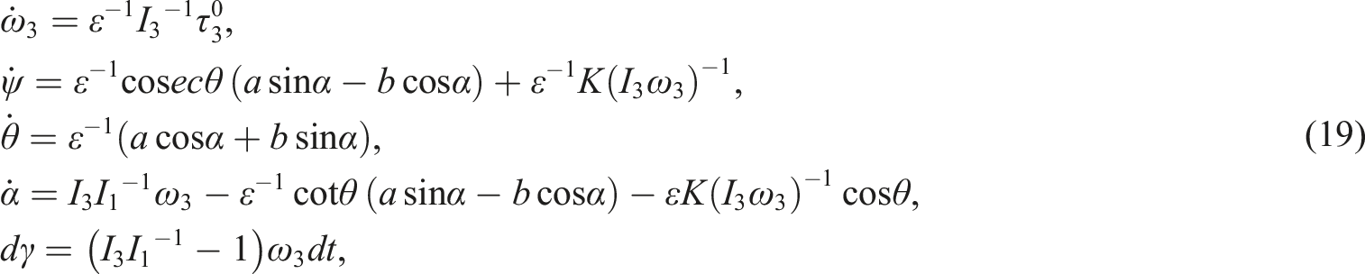
The considered motion in this case is described by Euler’s angles named: the nutation angle $\theta$ , the precession angle $\psi$ , and the pure rotation one $\varphi$ . We deduce from (32) and (31) that the angle $\theta$ of nutation is still constant for all $t$ over the motion, whenever the angle $\psi$ of precession contains the time $t$ .

For the approximation of order zero in ${\epsilon }^{-1}$ , we can deduce that

$\dot{\theta }=0,\dot{\psi }=0,\mathrm{a}\mathrm{n}\mathrm{d}\hspace{0.17em}\dot{\varphi }={{\omega }_3}_0.$

(34)

Therefore, the permanent rotation case in the equatorial plane is slow for the gyro motion about the symmetry axis $z$ is attained.

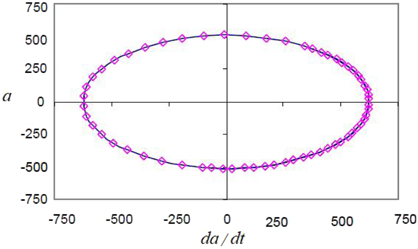
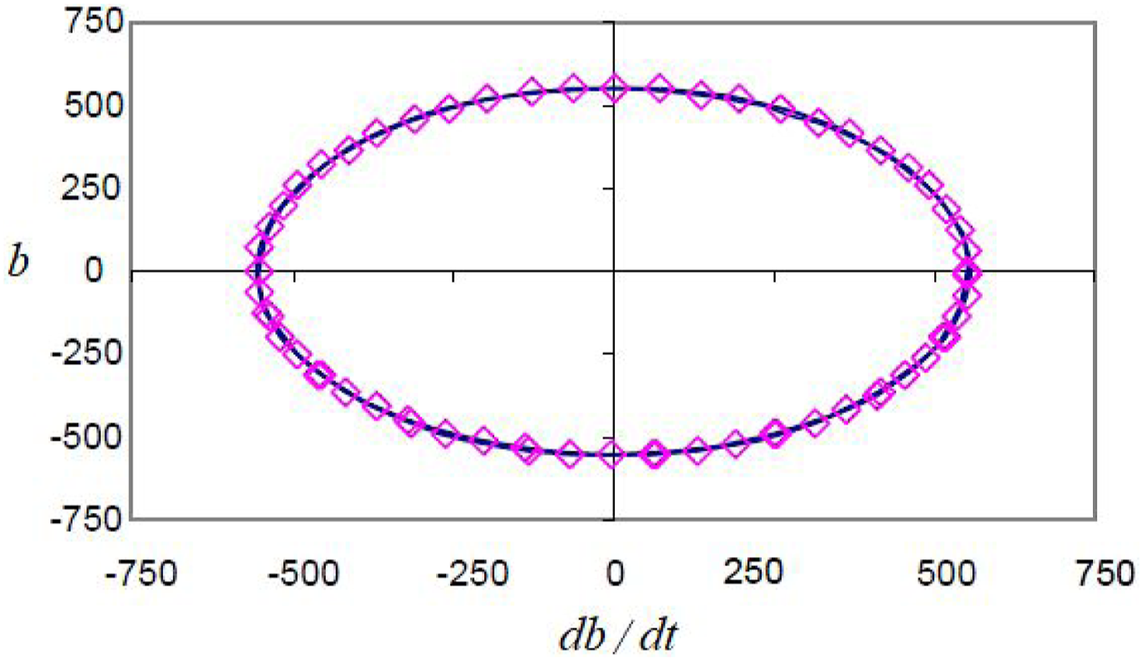
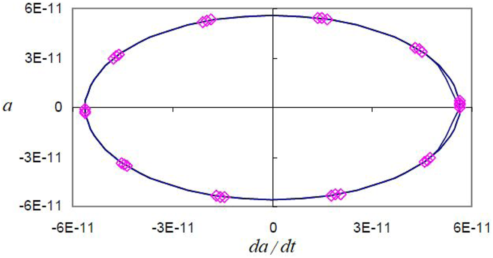
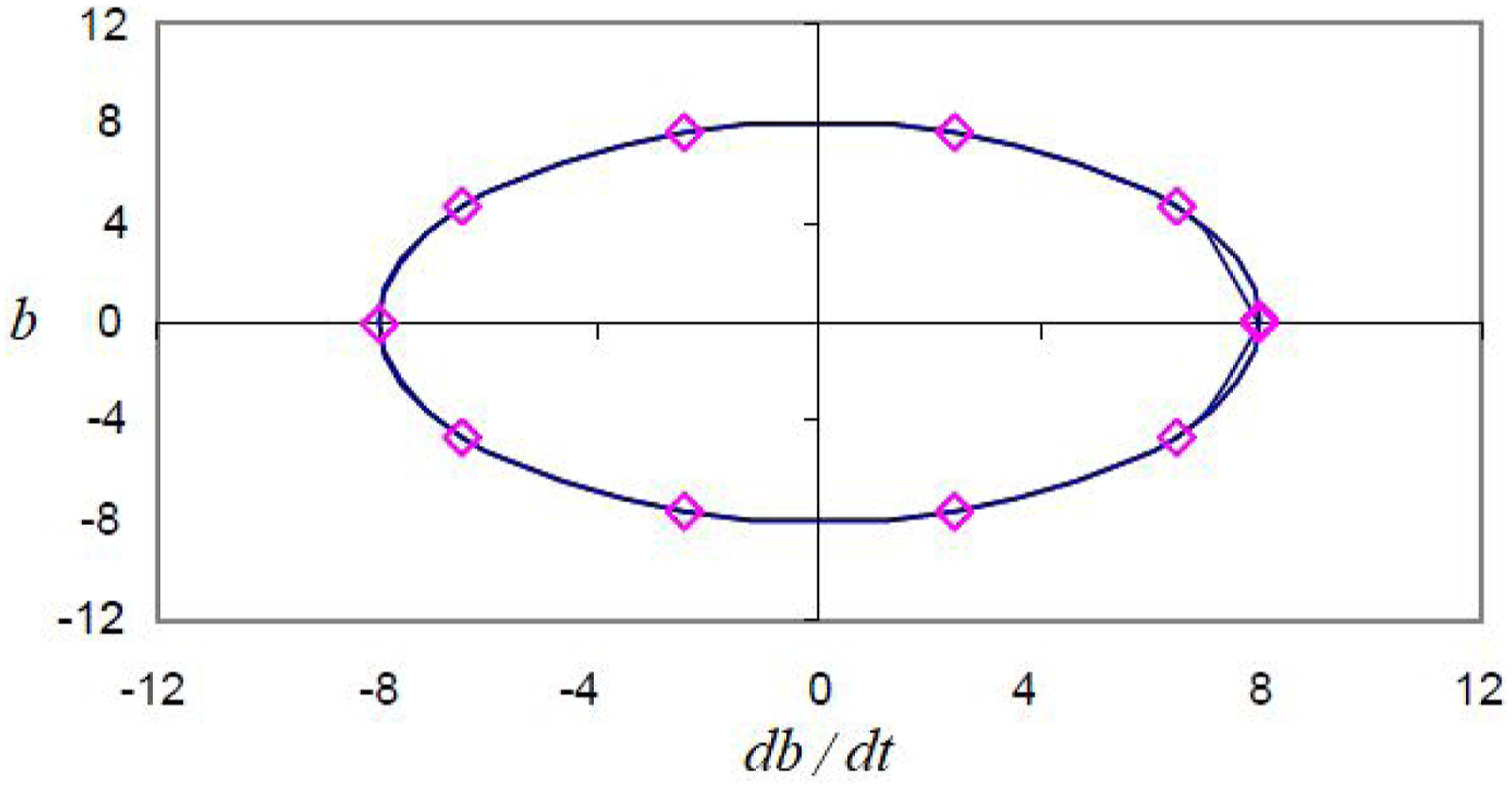
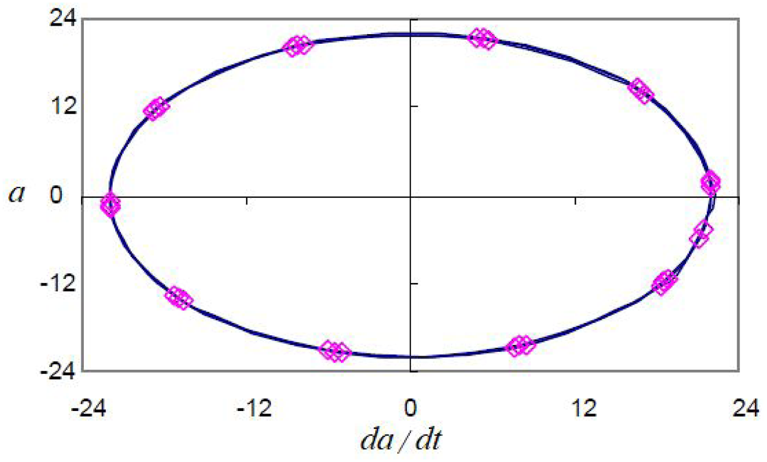
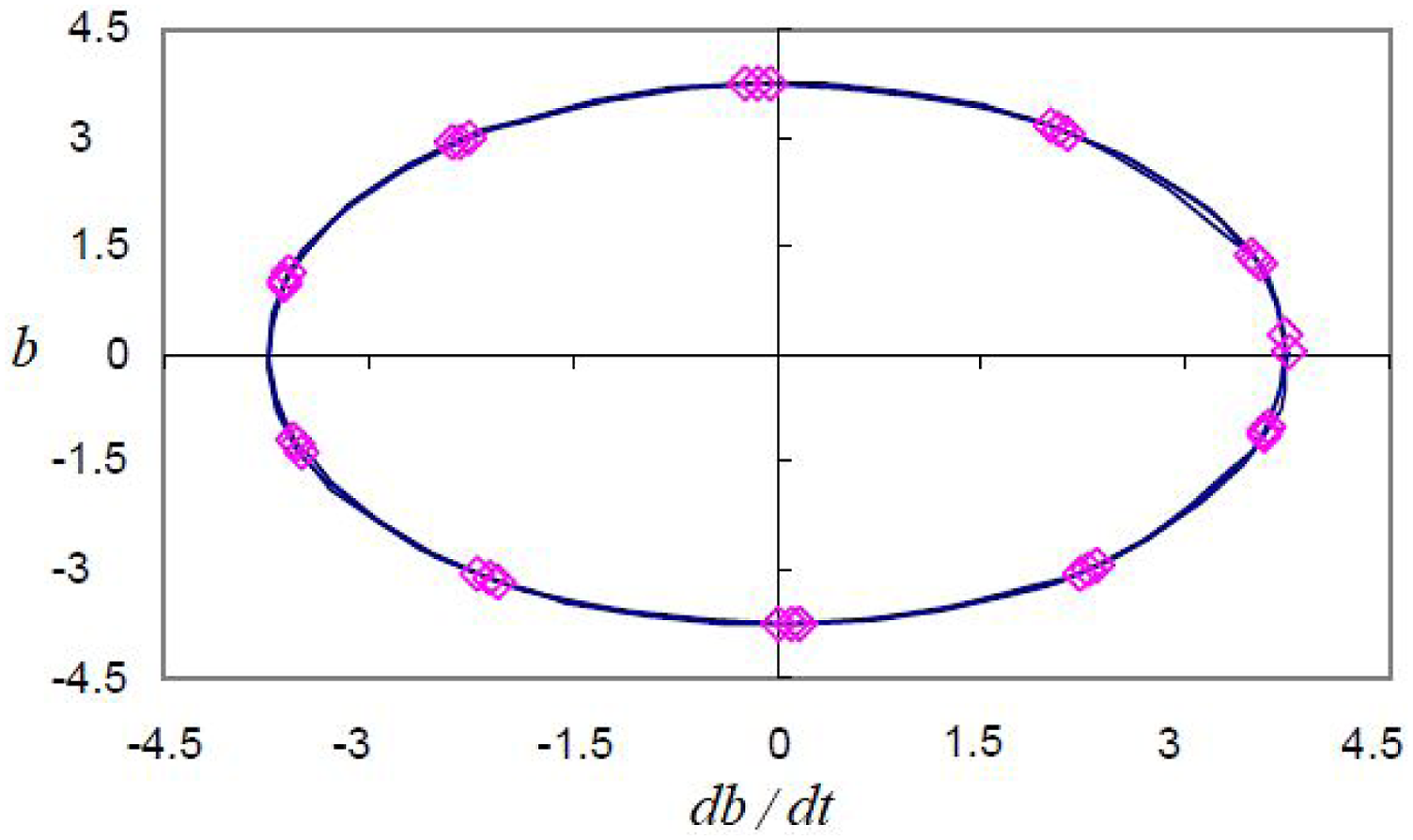
The study of the stability of the analytical and numerical solutions (a) and (b) for the point charge $Q\left(=\mathrm{100,3000,300}\right)$ Gausses is considered for both the analytical and numerical solutions and given through the phase diagrams in Figures 2–7, in which the blue and red curves represent the analytical and numerical results, respectively. From these diagrams, we show that the analytical and numerical solutions are stable for different point charge values and are in full agreement together. That is, the numerical solutions are analogous to the analytical ones for the different values of the point charge $Q$ . The motion permutation is slow because the existence of the stiffening force for a long-time $t$ . We also get a smaller value of the period’s argument.

Figure 2.

The stability diagram for the solution $a$ and $da/dt$ when $Q=3000$ .

Figure 3.

The stability diagram for the solution $b$ and $db/dt$ when $Q=3000$ .

Figure 4.

The stability diagram for the solution $a$ and $da/dt$ when $Q=100$ .

Figure 5.

The stability diagram for the solution $b$ and $db/dt$ when $Q=100$ .

Figure 6.

The stability diagram for the solution $a$ and $da/dt$ when $Q=300$ .

Figure 7.

The stability diagram for the solution $b$ and $db/dt$ when $Q=300$ .

Conclusion

A constrained vibrating motion of a coupled gyrostat with a spring has been examined. Along with the action of Newtonian and electromagnetic fields, the gyrostat has also been affected by the gyrostatic coupling vector. The gyrostat has been thought to rotate slowly around either the minor or major primary axis of the inertia ellipsoid. The large parameter technique has been utilized to derive periodic solutions of the gyrostatic EOM. A geometric depiction using Euler’s angles has been provided to assess and analyze the gyrostatic motion at any given time. Throughout computer programs, analysis of the acquired solutions is considered in terms of selected numerical data. To produce numerical solutions that demonstrate the reliability of the analytically computed periodic solutions, characterized parametric data are assumed by one of the numerical methods. Phase diagrams have also been produced for the obtained solutions aiming to describe their periodicity and stability processes in a manner like.^30,31 The considered large parameter technique gives us the chance to study the problem under new conditions which saves the used energy to move the body initially. It also enables us to investigate various problems in new areas of the gyrostatic motion and solve several complicated cases that never solved by the previous techniques.