This article studies the motion of a three degrees-of-freedom (DOF) dynamical system, which consists of two parts, a dynamic part, and an electromagnetic harvesting device. The composition of the system depends on the magnet oscillating in the coil of this device. An electric potential is exerted because of the electromotive force to obtain energy harvesting (EH). Lagrange's equations (LE) are used to derive the system’s equations of motion (EOM), which are solved analytically up to a third-order of approximation using the multiple-scales method (MSM). These solutions are considered novel, in which the mentioned method is applied to a novel dynamical system. The gained are confirmed through comparison with the numerical solutions of the EOM to reveal a high degree of consistency. To establish the system’s solvable conditions and modulation equations (ME), three scenarios of primary external resonance are investigated simultaneously. Certain diagrams of time histories for the amplitudes and phases of the examined dynamical system are plotted to show their behaviors at any given instance of time. The Routh–Hurwitz criteria (RHC) are used to establish the stability and instability regions in light of the graphs of resonance response curves. The presence of an energy harvester in dynamic devices helps us to convert vibrational motion into electrical energy that can be exploited in several applications in a variety of daily tasks, including structural and environmental monitoring, military applications, space exploration, and remote medical sensing.
It is known that non-renewable energy is running out rapidly and will be depleted over the coming decades. Therefore, it is very necessary to change the type of energy production and create renewable, clean energy sources. We can also use so-called EH, in which it is difficult to use large batteries to replace them regularly in portable and wireless systems, so we resort to compact and efficient power sources that enable us to increase the use of wireless devices. Therefore, the best possible idea for using energy in small systems as the main source is EH. Thus, using available energy resources, temporary power tanks can constantly be replaced with charged energy storage elements, including sunlight, heat, and vibration.1–3 Vibration is particularly charming because of its many uses. Vibration sources are available in environments such as vehicles and human movements.
Energy is harvested from electromagnetic, piezoelectric, or electrostatic transmission. Also, these vibrations often occur at low frequencies, which means that the energy levels are low at the output. The amount of energy produced by such systems is in the micro to milliwatts order.4–10 Electromagnetic energy originates from Faraday's law of induction11 since any change in the magnetic environment of a wire coil induces an electromotive force in the coil. This occurs according to the motion of the magnet relative to the coil.12 Capacitors are used in electrostatic transformation to convert mechanical energy into an electric field, which may be employed to provide current to an electric circuit.13 When a piezoelectric material is deformed under stress, an electric field is generated, and a voltage is produced.14 In Reference 15, the authors demonstrated the study of vibration reduction and EH in a dynamic system of a spring pendulum. In Reference 16, the spring pendulum system was connected to two different EH devices, each in a separate case, in which the controlling EOM were obtained. Moreover, the ME were determined in light of the classification of the examined resonance cases. It is generally acknowledged that mechanical systems, especially vibrational dynamics problems such as References 17–20 are regarded as the most significant problems in mechanics due to their broad spectrum of applications, particularly in engineering. In Reference 17, a general model composed of a nonlinear, damped, excited spring pendulum is studied. Its suspension point was restricted to moving in an elliptic trajectory with a stationary angular velocity, while its other end was connected to a rigid body. For both the numerical and approximate solutions, the time-varying histories of the resulting solutions are displayed. Whereas in Reference 18, a 3DOF nonlinear system was investigated, in which LE were used to derive the governing EOM and solved analytically by applying the MSM method.19 Curves of frequency response were graphed to show the influence of the system’s parameters on the stability and instability areas. The chaotic motion of a spring pendulum under the action of a harmonically excited force was investigated in Reference 20. The authors considered that the planar motion of its pivot point was in a circular path. The positive effect of a viscous fluid on a pendulum spring was studied in Reference 21 when the suspension point was stationary, where buoyancy, drag, lift, and external forces were considered.
Systems for EH in dampening vibrations have been examined in References 22,23. It is an electromagnetic harvester attached to the automatic parametric pendulum that acts as the absorber. The overall performance of a combined damping vibration was studied, and it was shown that this combination did not reduce the vibration-damping efficiency. It was observed in Reference 22 that energy could be harvested for the rotation and chaotic motion of the pendulum. In Reference 23, a pendulum system with two independent electromagnetic harvesters is presented. A direct-current motor is added to the swing shaft to serve as a second harvester. The results showed that the proposed system significantly improves the capacity of EH, and the efficiency of vibration suppression for rotary harvesters is low. In Reference 24, vibration absorbers were developed as energy-harvesting devices and vibration-damping systems to suppress undesired vibrations and generate induced voltages that can be used in low-voltage applications such as wireless sensors. In Reference 25, a numerical analysis of a semi-active suspended vibration absorber, or harvesting system, was performed. The primary objective was used to dampen the vibrations of the primary structure, and the secondary objective was considered an absorber that simultaneously harvested energy from the vibrations. The pendulum-tuned mass absorber was regulated by a magnetic levitation collector. The influence of EH, and the control of vibrations by specially designed pendulum dampers, and the use of nonlinear dampers as energy harvesters were studied in Reference 26. The use of energy recovery devices has been shown to provide better vibration reduction in the low-frequency range. In Reference 27, the authors present a new pendulum absorber harvester structure that improves vibration suppression and EH characteristics. The damper configuration of the system refers to the use of magnets, whose performance was studied empirically and theoretically. The results showed that the new damper harvester has greater performance than the traditional device with both oscillation suppression and EH. The movement of a 3DOF dynamic system, which creates an auto-parametric model, is examined in Reference 28. In addition to evaluating stable and unstable zones, the authors used the nonlinear stability approach to investigate the system’s frequency response curves. In Reference 29 the authors analyzed a piezoelectric energy harvester under synchronous resonances. The obtained results showed that the generated voltage and power level are amplified under the simultaneous effects of two strong excitations such as super-harmonic and harmonic resonances. Energy harvesting and Wideband vibration isolation based on a coupled piezoelectric-electromagnetic structure were investigated in Reference 30. Using energy harvesting to power marine environment monitoring was studied in Reference 31. In Reference 32, the vibrational motion of a 3DOF dynamical system connected to an electromagnetic EH device is studied, which converts the vibrational motion to electric energy. The motion of a nonlinear damped dynamical system with a piezoelectric transducer is investigated in Reference 33. The bifurcation diagram, Poincaré diagram, and Lyapunov exponent spectrum are presented. Moreover, three different motion modes of the system, which are quasi-periodic motion, hyperchaotic motion, and chaotic motion, are examined. It is worth noting that high output voltage and power are obtained by controlling the values of natural frequency, excitation amplitude, capacitance, coupling coefficient, load resistance, and damping coefficient.
In this paper, we demonstrate a simple device based on spring vibrations to harvest energy from a vibrating environment, which converts the vibrating mechanical energy into an electrical one. The studied system is composed of two connected masses with two damped springs. One of these masses moves horizontally, and the second one has a planar motion in view of the existing EH device. This system is acted upon by two external forces and one moment. The MSM is utilized to obtain novel approximate solutions that fit the generalized coordinates of the regulating system of the EOM. The emerging resonance cases are grouped, in which three of them are examined at once, and then the ME are established based on the examined resonance situations. When the stability of the system is examined by using RHC, several areas close to resonance ranges are plotted to assess the dynamic frequency response curves for various values of the acting parameters. The realized solutions are plotted for the same values of these parameters to observe how the system’s motion behaves. The various values of the excitation amplitudes, damping coefficients, and load resistance are displayed as functions of the output current time series and power. The results of this work can be used in a variety of applications, including automotive,34 health monitoring devices,35 wireless sensor networks,36 and civil engineering.37
Description of the dynamic system
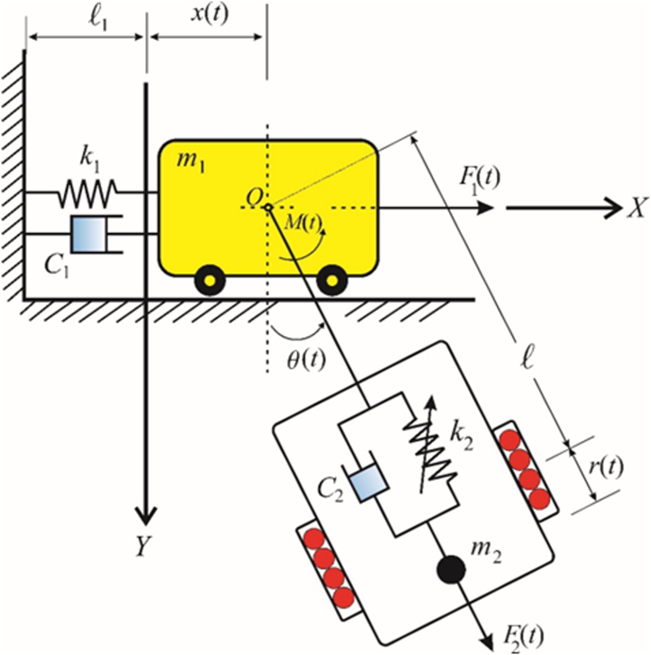
This section describes the investigated system, which consists of two parts: a dynamic part and a harvester device. The dynamical part consists of masses connected with two damped springs of normal lengths and linear stiffness coefficient , and damping coefficients besides , see Figure 1. One of these masses is directed horizontally, and the other has an angle of rotation . An EH device is located at the damped spring of mass . The construction of this system can be estimated according to the magnet's oscillation within the coil of this device. As a result, an electric potential is generated through electromotive force, which is harnessed to harvest energy. It is hypothesized that the dynamical motion of this system is impacted by the external harmonic forces (in the horizontal direction), , (along the pendulum’s arm) and the moment (at the point ), in which and represent the amplitudes and frequencies of the acted forces and moment, respectively. The harvester is coupled with the spring of mass , which consists of two magnets that are fastened to the end of a cylindrical tube.
The dynamical system.
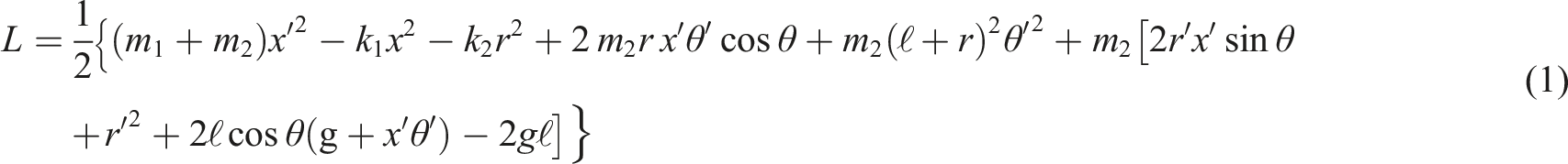
Due to the fact that any dynamical system has a Lagrangian , where and represent the system's kinetic and potential energies, respectively. In accordance with the examined system, it is possible to write
Here, dash represents the derivatives regarding time while and are the system’s generalized velocities.
Based on equation (1), the following Lagrange’s equations can be identified to determine the governing system EOM
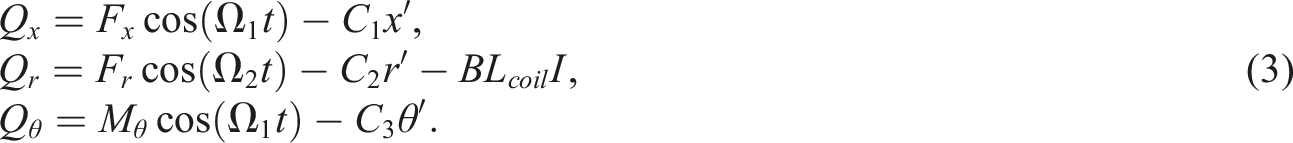
where are the forces that have been applied generally to the dynamical system under investigation, and they take the following forms
Here, is the generating current, refers the coil length and is the magnetic flux.
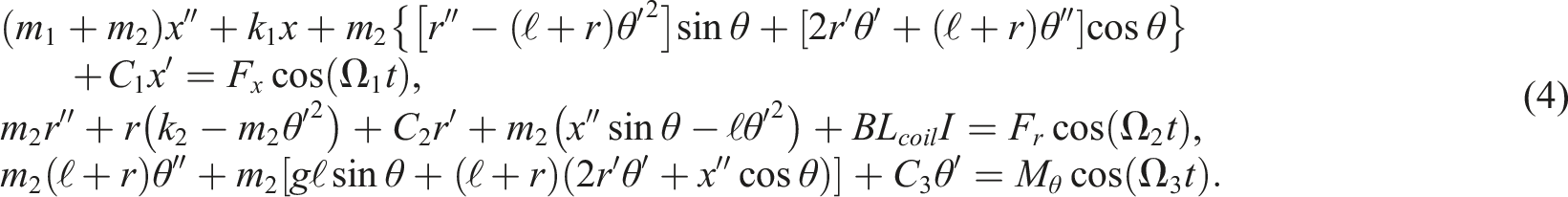
Substituting equations (1) and (3) into equation (2), we can write the EOM as follows
For the electrical circuit, we can write the Kirchhoff Voltage law and Faraday's one of electromagnetic induction.11
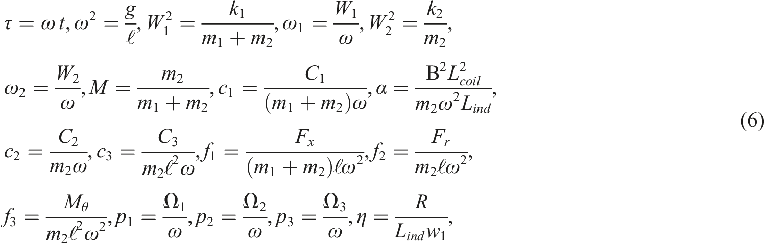
where denotes the total of the resistances of the coil and the load . Let us insert the below dimensionless parameters
besides the dimensionless coordinates and .
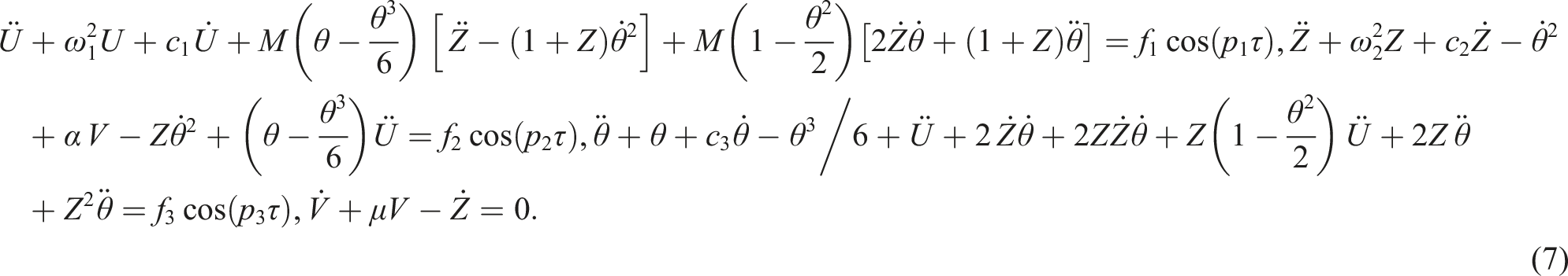
Making use of the aforementioned parameters (6) and equation (5), one can rewrite the system (4) in their non-dimensional forms as follows
Here, dots are the derivatives regarding . The aforementioned system is categorized as a nonlinear second-order differential system.
The proposed perturbation method
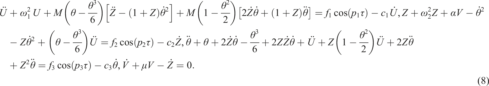
The major purpose of this section is to use the MSM to achieve the essential approximate solutions for the EOM of the previous systems (7) up to higher-order approximations. To achieve this aim, the functions and in system (7) can be approximated using Taylor series until the third-order of their expansions, which are valid in an extremely small region surrounding the position of static equilibrium.38,39 Therefore, system (7) can thus be rewritten as
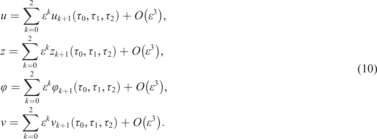
We suppose that the generalized coordinates can be represented in terms of tiny parameter . As a result, we look at three additional variables, and , as shown below
In accordance with the MSM, one may construct the functions and in powers of as19
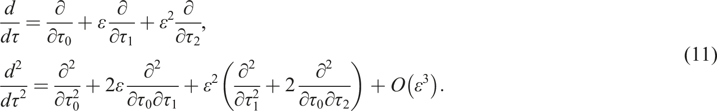
Here symbolize various time scales, with and are, respectively, defined as fast and slow scales. Consequently, the chain rule shown below may be employed to transform the -varying derivatives of as
It is important to recognize that terms beginning with and higher are careless due to their smallness.
To achieve the required solutions, the amplitudes , damping coefficients , and the parameter might be specified as
Substituting (9) - (12) into (8) and equaling coefficients of different powers of in both sides to get the below three groups of partial differential equations (PDE)
Order of
Order of
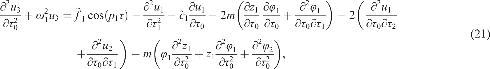
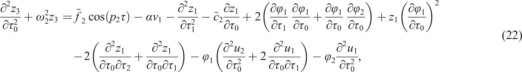
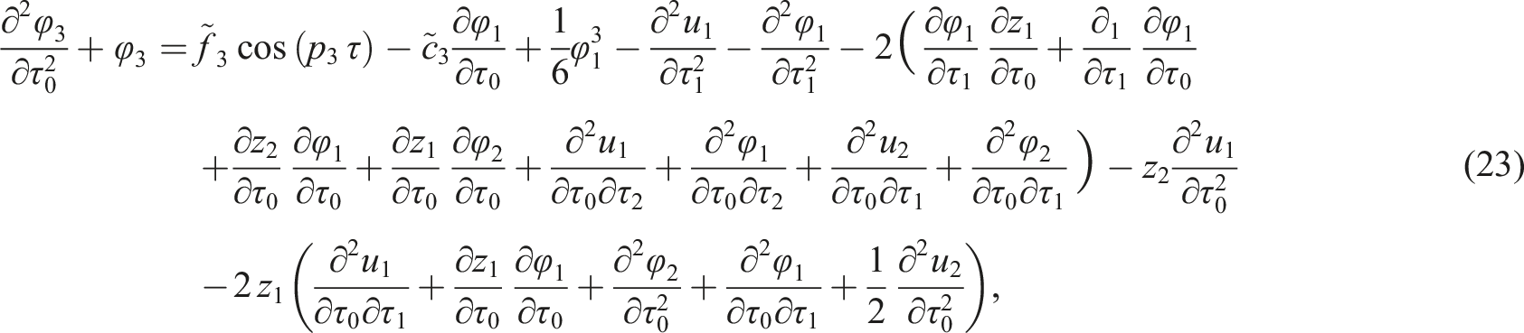
Order of
It is interesting to note that the forgoing equations (13) to (24) are of orders comprise 12 PDEs that can be solved consecutively. To accomplish this goal, let us start with the following general solutions of the homogenous equations (13) to (16)
The substitution of (26) into equation (16), yields a PDE that can be solved to have the form
Here and are undetermined complex functions, while are the related complex conjugates.
Substituting the first-order solutions (25) to (28) into the PDE of the second group (17) and (20) and then cancelling the emerging secular terms to get the second-order solutions as follows
where means the complex conjugates of the preceding terms.
Using the four equations provided above, we can determine the prerequisites for deleting secular terms from the second approximation as follows
where the functions and depend on only.
The third-order solutions can be obtained by substituting (25) and (28) and (29) and (36) into (21) and (24) besides the removal of secular terms. The following conditions must be met to cancel these terms
where
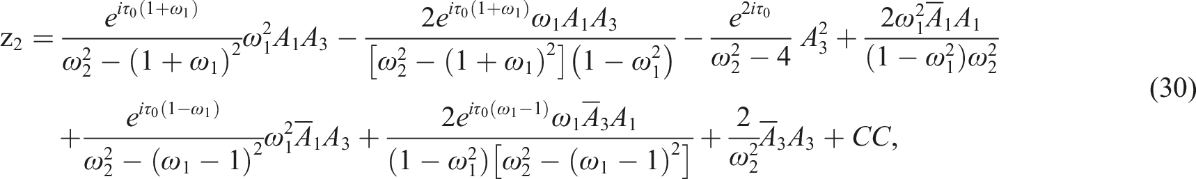
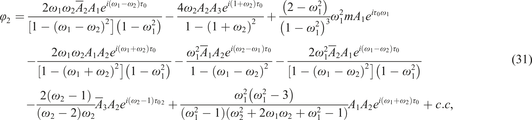
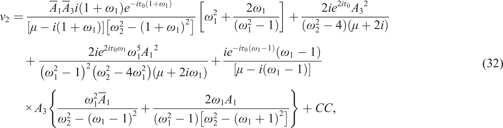
Moreover, the third-order approximations have the forms
The main topic of the current section is to classify the evolving resonance cases. These cases could arise when the denominators of higher approximations equal null.36 Therefore, according to second and third approximations (29) and (32) and (43) and (46), one may obtain the following resonance cases
(a). Internal resonance occurs when one of the next conditions is satisfied
(b). When there is a chance for external (primary) resonance.
It should be noted that the behavior of the studied system will be quite challenging if any one of these conditions is met. Additionally, the approximate solutions achieved above will still hold if the oscillations have values that are not very similar to the resonance situations. To examine the stability of the system, the requirements of solvability and ME for this system must be obtained. Consequently, we will simultaneously examine the three cases of primary external resonance. Specifically, we take into account and that expresses how close and are to and , respectively. Following that, we add the detuning parameters as follows
We are now in the process of obtaining the solvability conditions. For this purpose, substitute (47) into the PDE equations (27) and (19) and (21) and (23), then eliminating the secular terms, the conditions of solvability can be gotten easily as follows
- For the PDE of the second-order of approximation
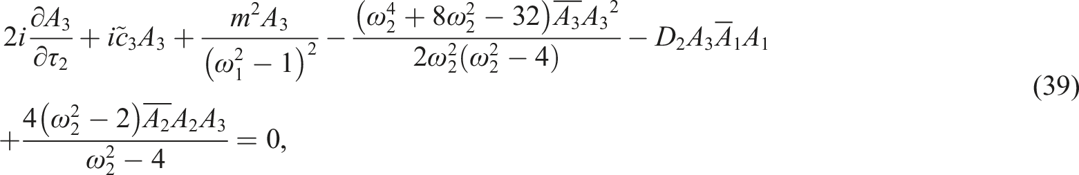
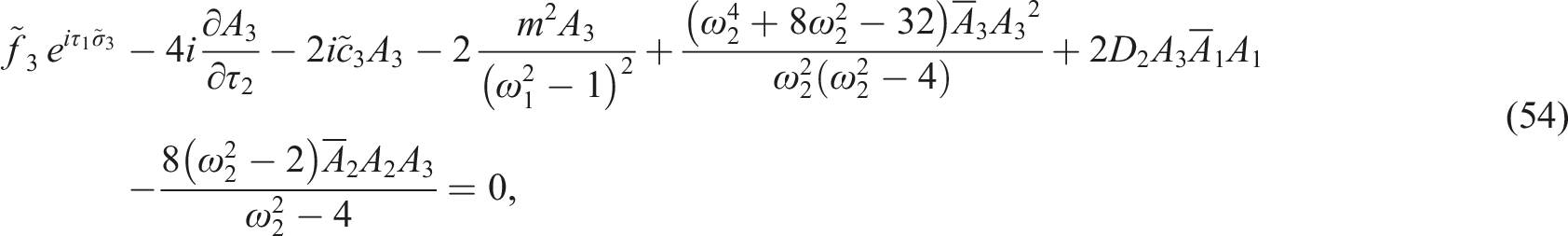
- For the PDE of the third-order of approximation
From the equations (55) and (51), we can express in the form
where is an unknown complex function of the higher slow time scales than .
We may identify the functions , which depend exclusively on , by using the previously solvability requirements (52) to (54). As a result, we take into account the polar forms as follows
Here and express the amplitude and phase of the solutions and . Consider the below adjusted phases
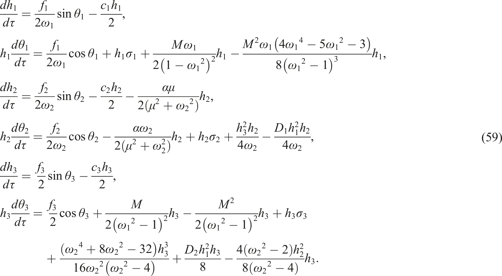
Making use of (57) and (58) into (52) to (54), and then separating the real portions and the imaginary ones to get the following ME
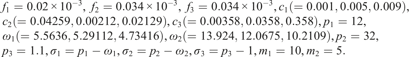
The previous autonomous system ME (59) consists of six ordinary differential equations (ODE) of adjusted phases and amplitudes . These equations can be solved numerically through the planes with the initial conditions and . These solutions are graphed in Figures 2, 3, 4, 5, 6, 7, 8, 9, 10, 11, 12, and 13 for a few different values of the system's dimensional parameters as and dimensionless parameters, that in accordance with the following data
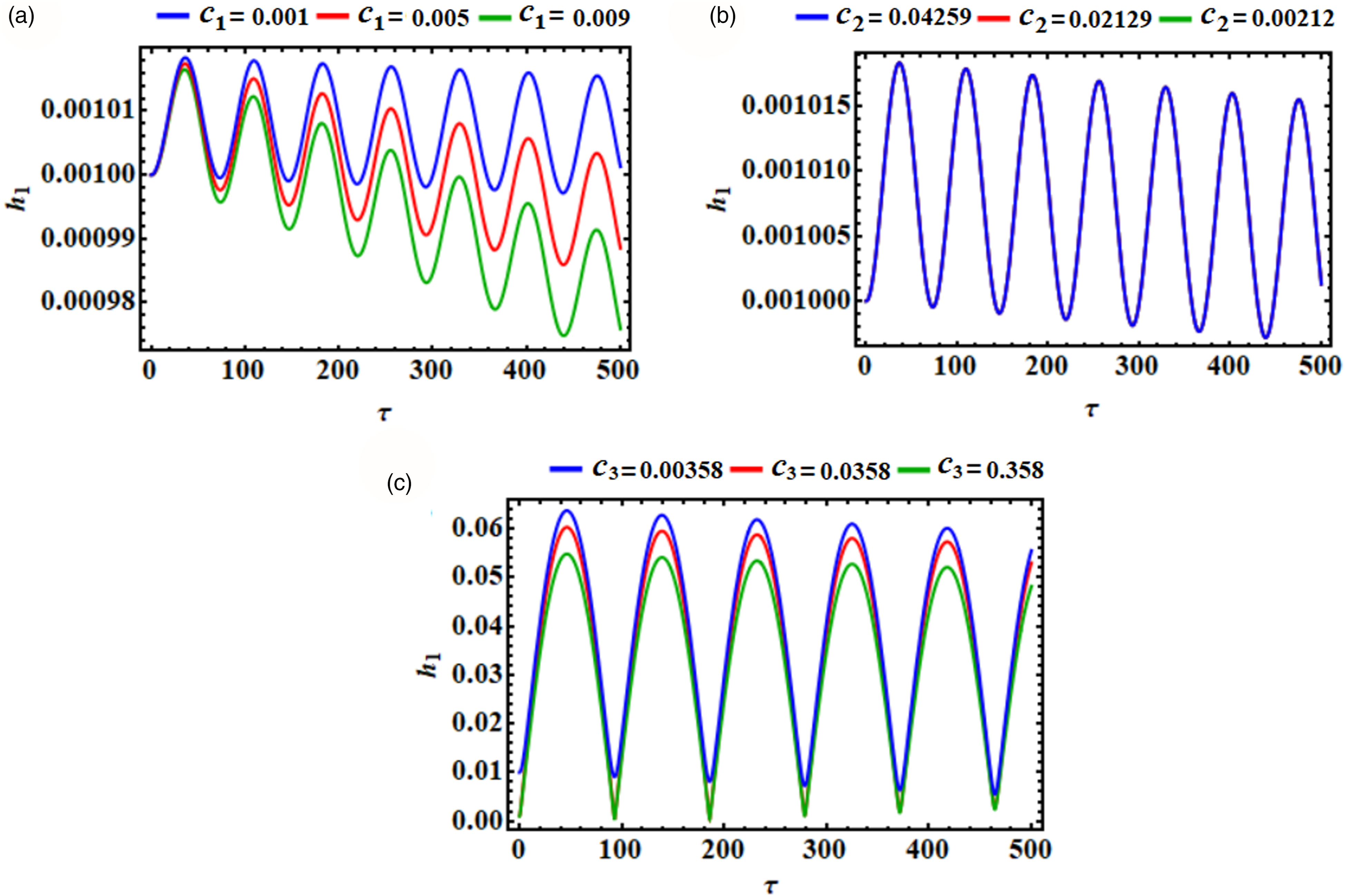
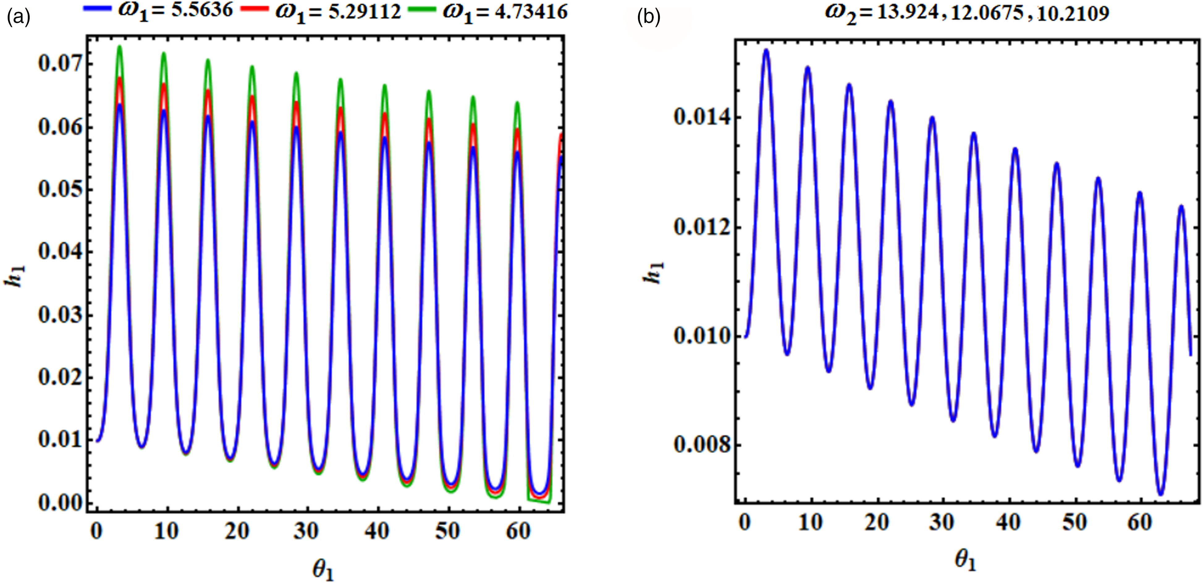
Presents the waves of at and for various values of: (a) , (b) , and (c) .
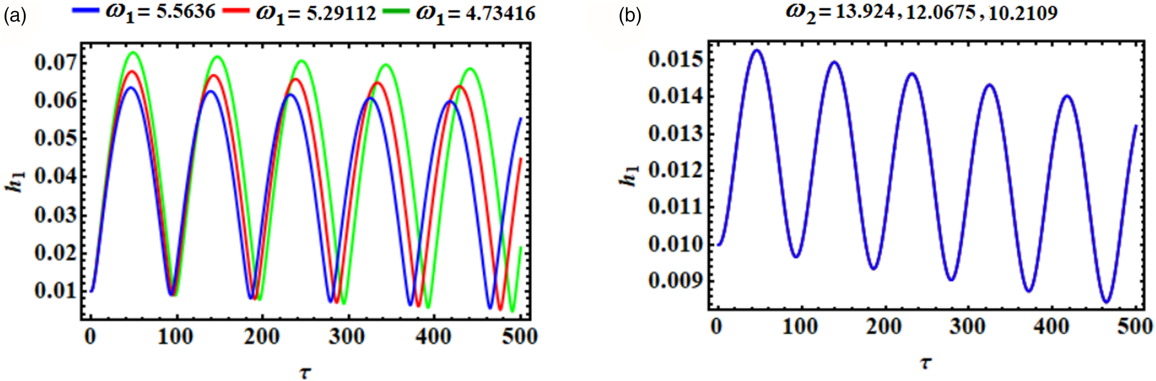
Shows the waves of at and for various values of: (a) , and (b) .
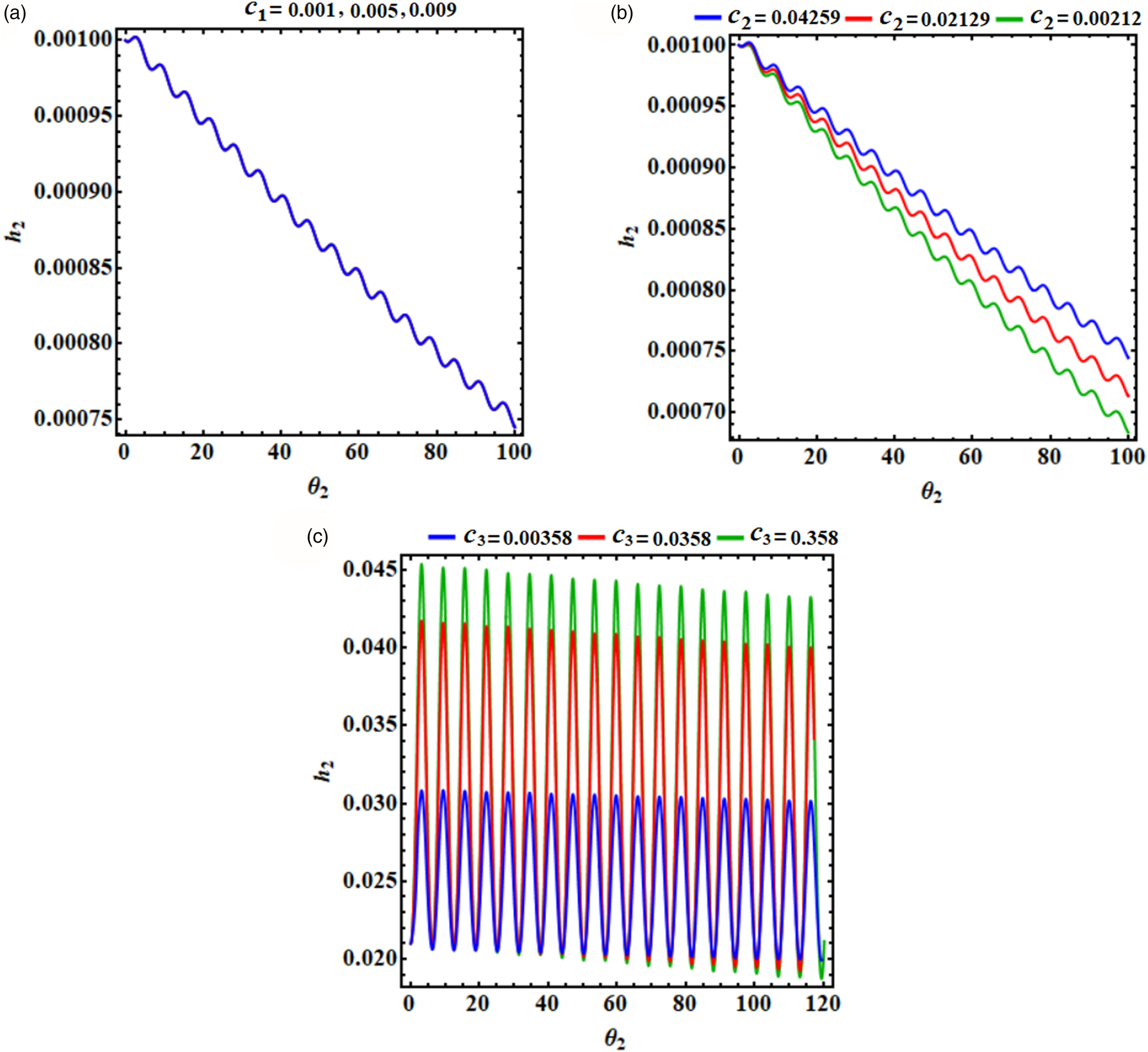
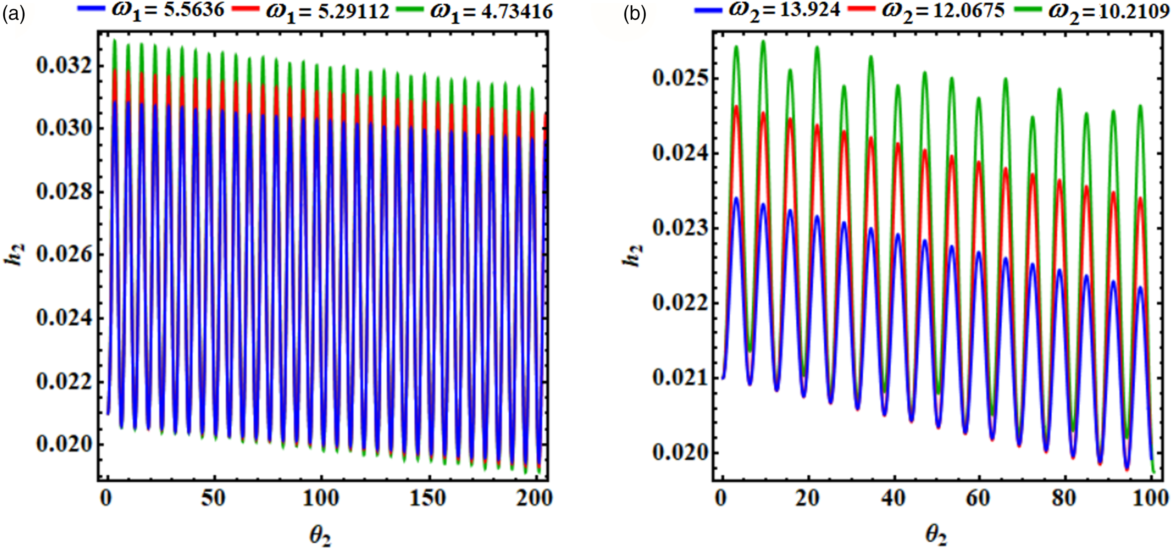
Presents the waves of at and for various values of: (a) , (b) , and (c) .
Shows the waves of at and for various values of: (a) , and (b) .
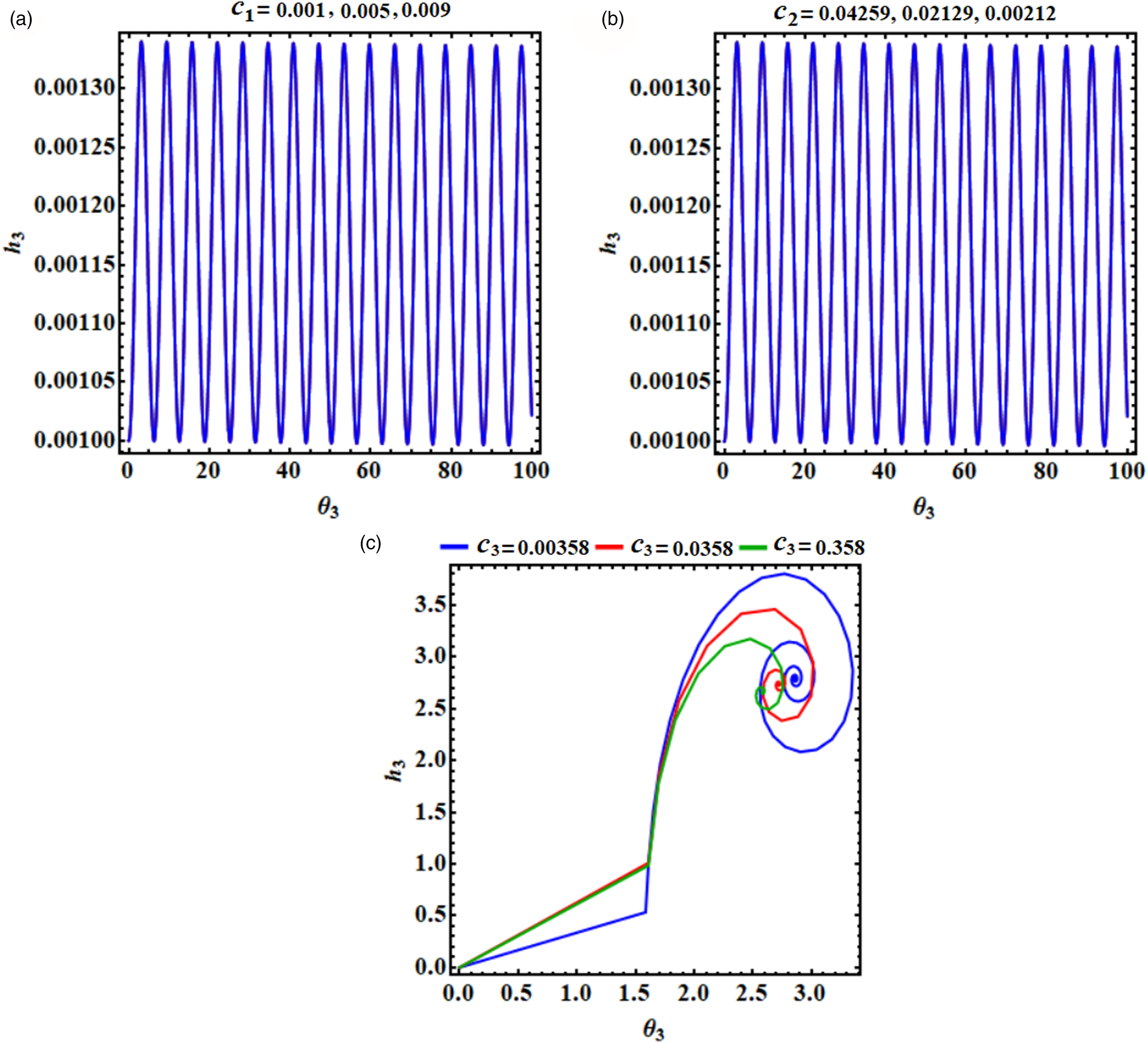
Illustrates the waves of at and for various values of: (a) , (b) , and (c) .
Presents the waves of at and for various values of: (a) , and (b) .
Describes the waves of at and for various values of at and for various values of: (a) , (b) , and (c) .
Presents the waves of at and for various values of: (a) , and (b) .
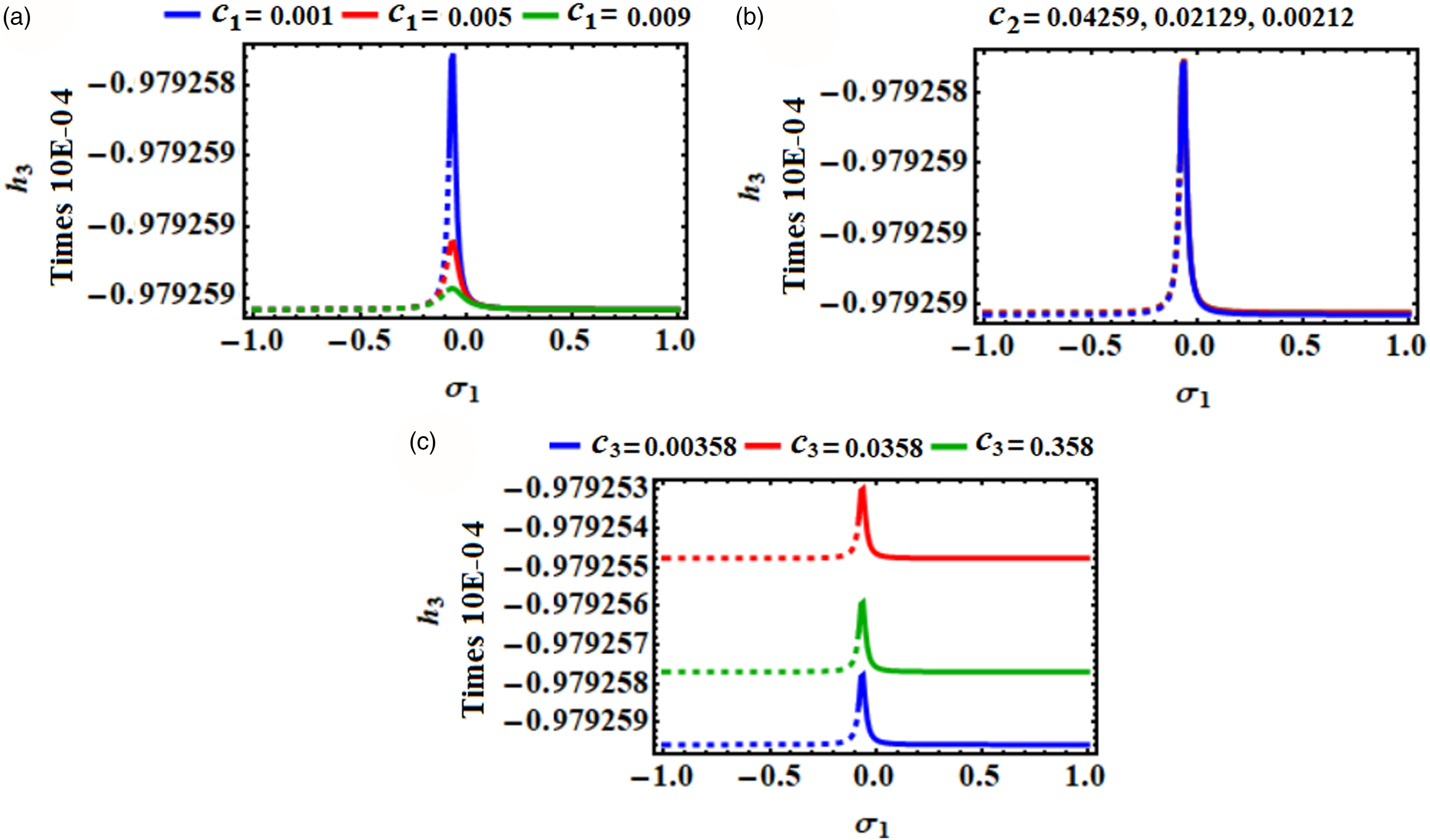
Reveals the behavior of at and for various values of: (a) , (b) , and (c) .
Presents the behavior of at and for various values of: (a) , and (b) .
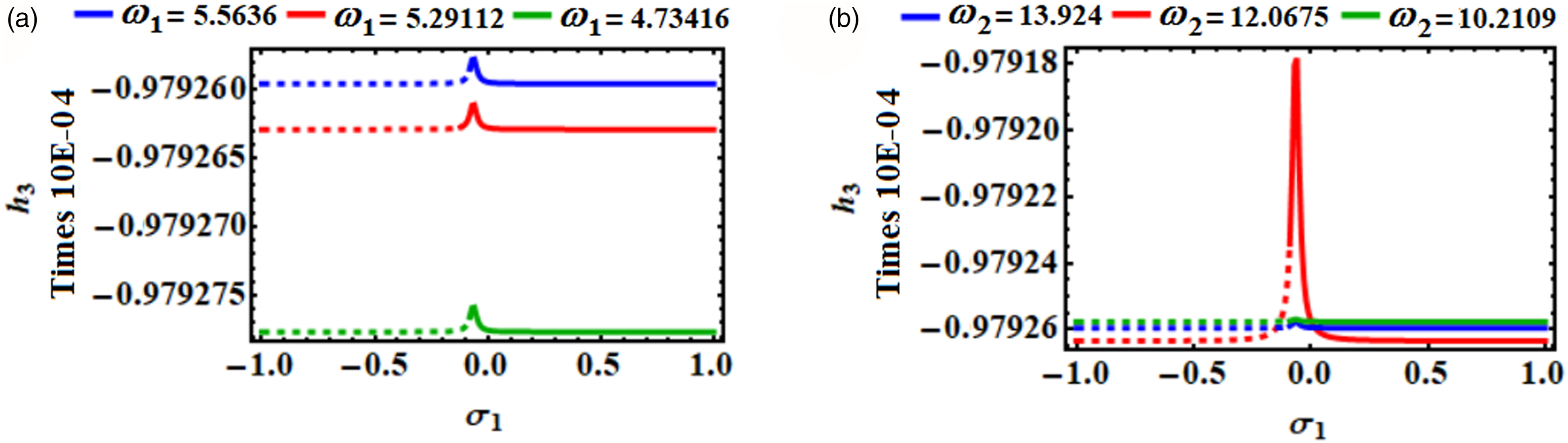
Presents the waves of at and for various values of: (a) , (b) , and (c) .
Presents the waves of at and for various values of: (a) , and (b) .
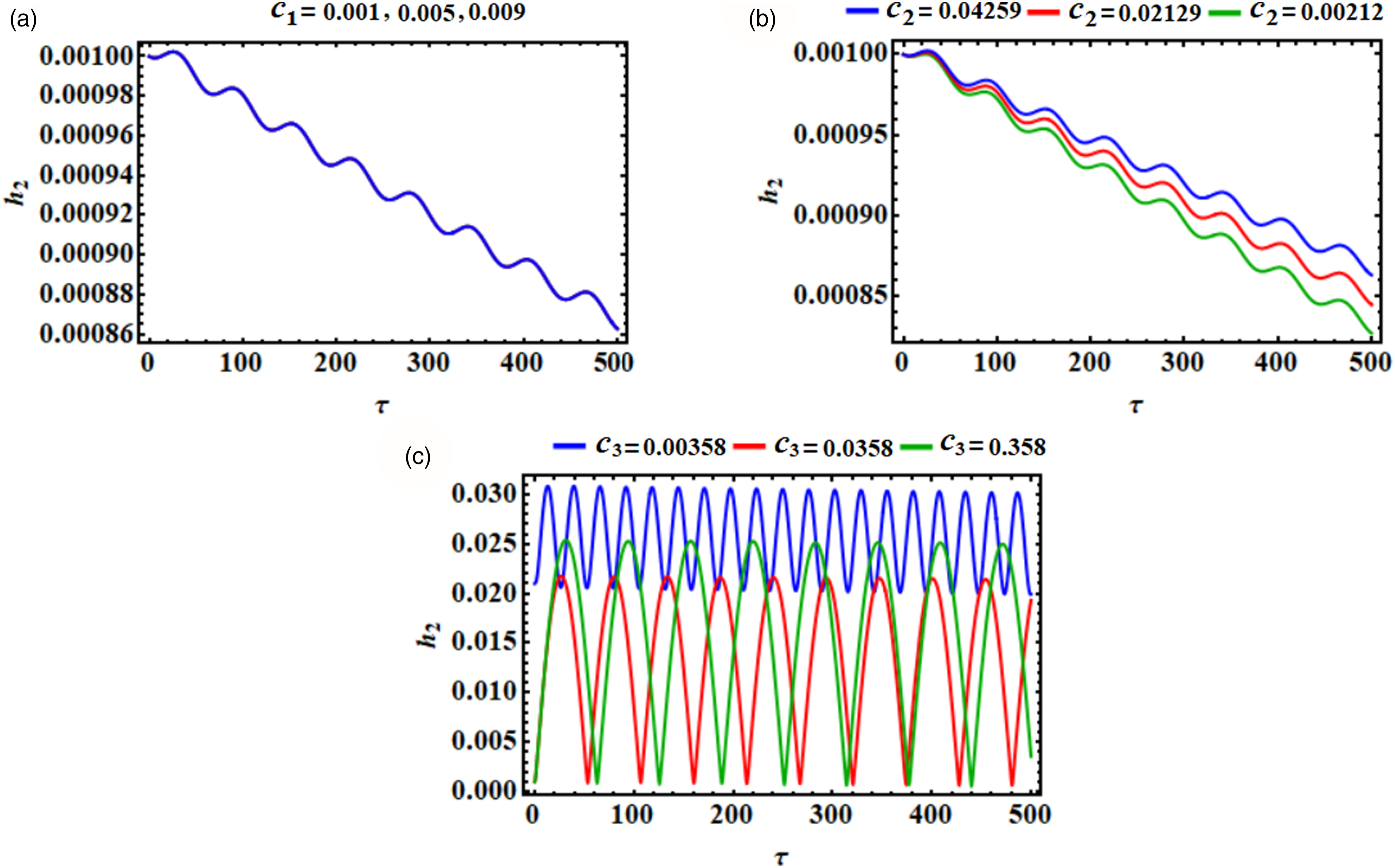
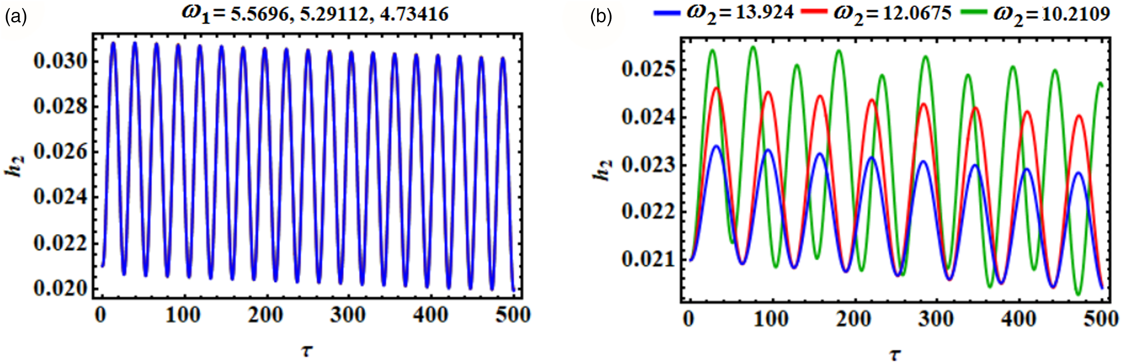
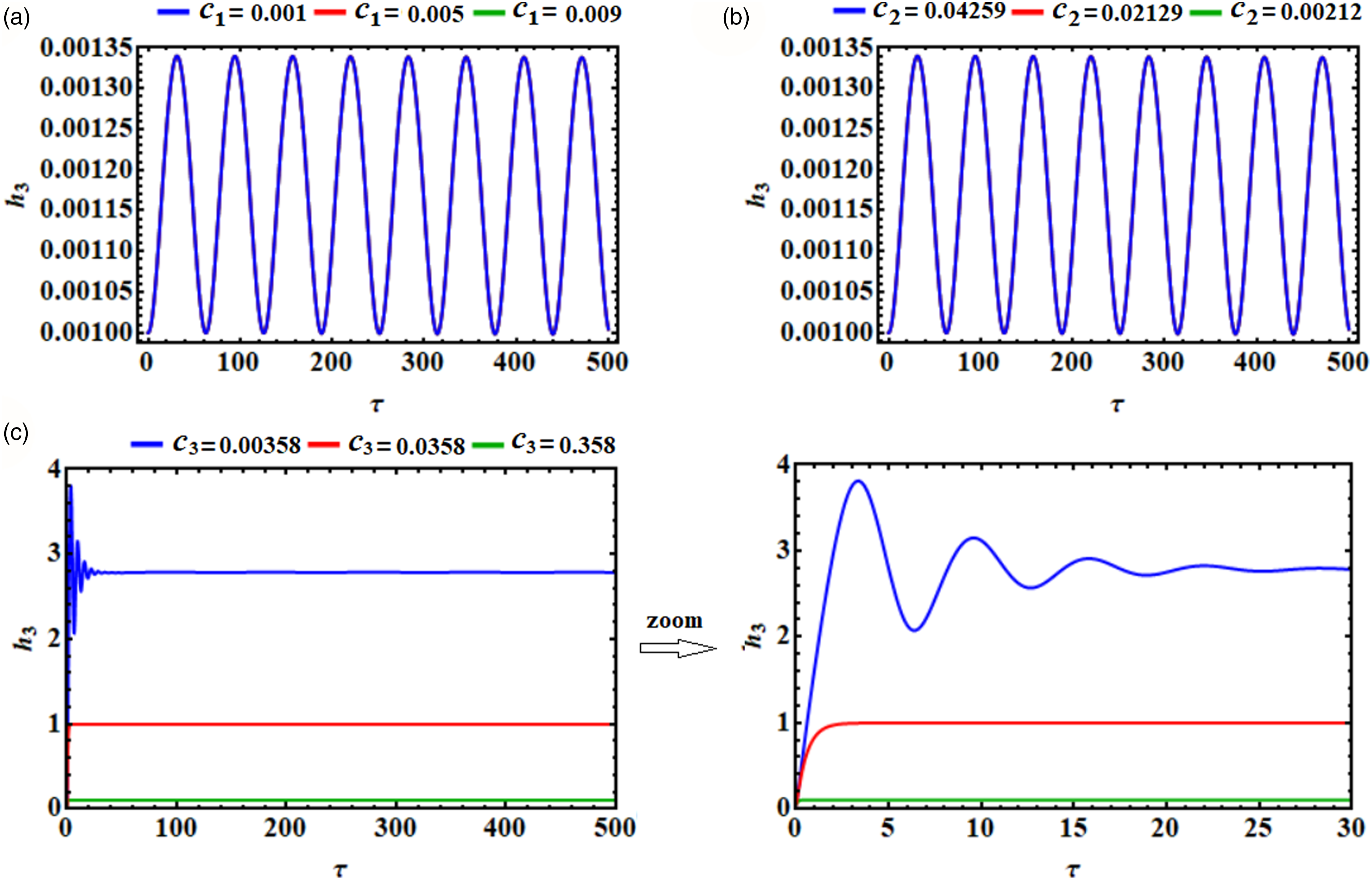
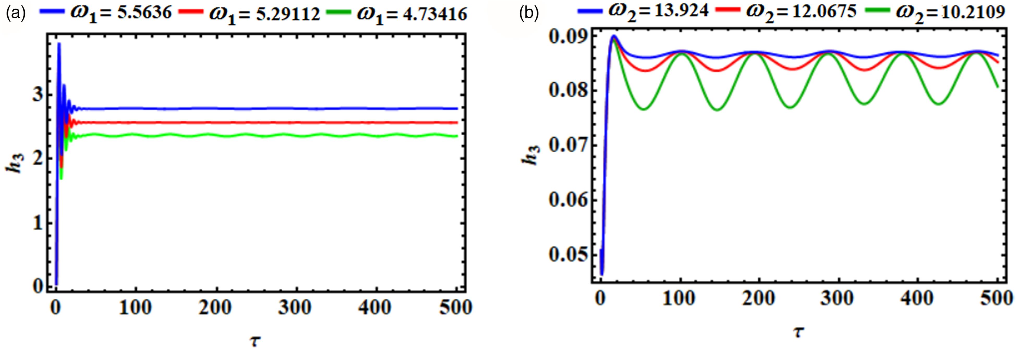
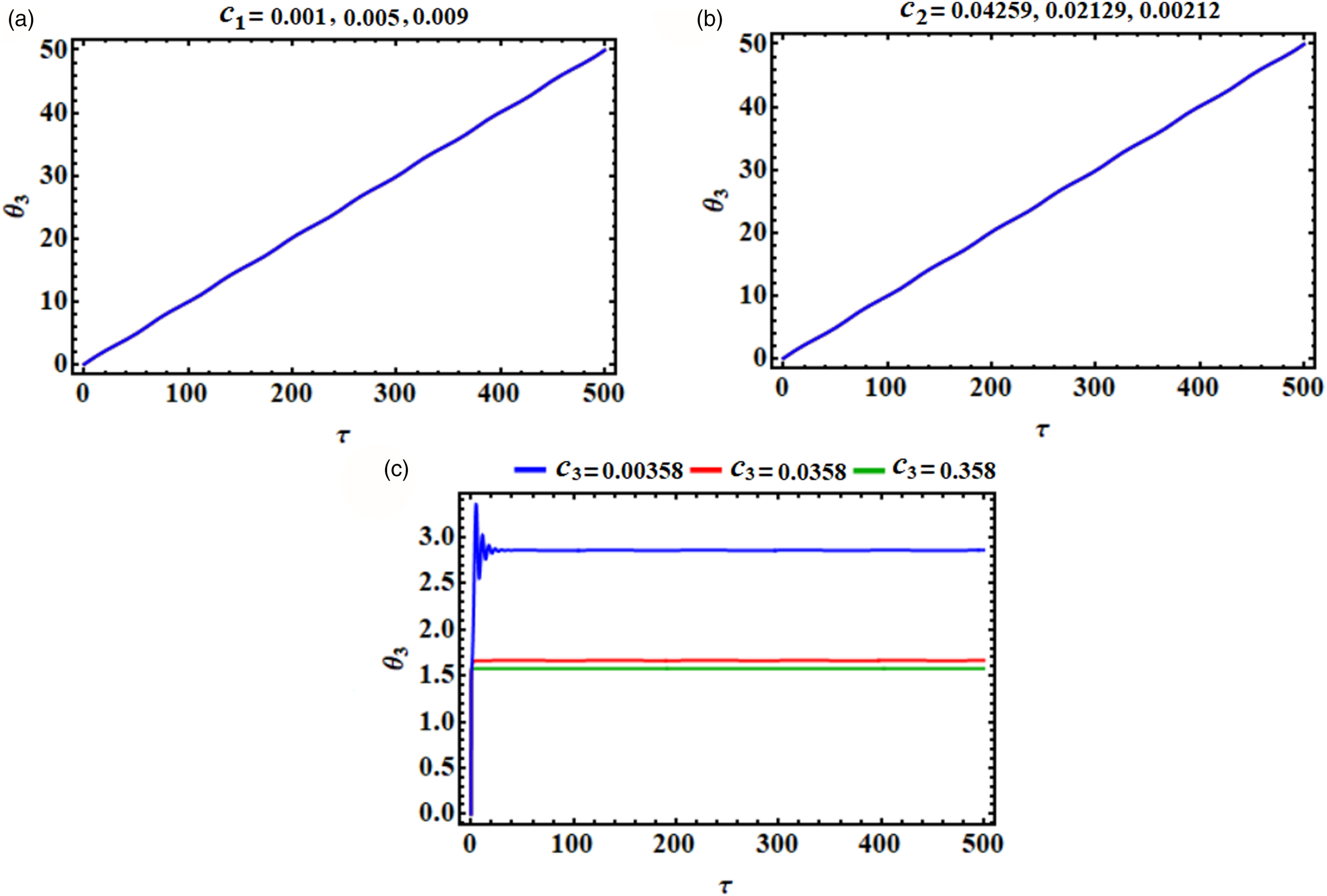
To examine the significance of acting parameters such as and on the behavior of the system, Figures 2, 3, 4, 5, 6, 7, 8, 9, 10, 11, 12, and 13 are plotted. These figures reveal the transient responses of the amplitudes and modified phases for system (59) of the above-mentioned specific values. Generally, one can note that the drawn curves in Figures 2, 3, 4, 5, 6, and 7 have decay manner over the examined time interval which reveals that the behaviors have stable procedures, while curves have various behaviors, as explored in Figures 8, 9, 10, 11, 12, and 13.
The curves in Figure 2 are drawn when the damping coefficients have different values and reveal the time variation of the amplitude over the time interval . The decay behavior of these curves during this interval is expected from the structure of the dynamical system (59) of ME. It is observed that the plotted waves have low impulses with the variation of and , as seen in Figures 2(a) and (b)) in which the waves’ amplitudes decrease with the increase of and . On the other hand, there is no variation of the wave when has various values, as seen in Figure 2(b), which is due to the fact that the related equation does not depend on directly. A closer examination of the graphed curves in Figure 3 shows that they are calculated when of and take various values. It is noted that the values of have positive impact on the curves of modified amplitude , as seen in Figure 3(a), while the values of have no influence on the wave manner, as explored in Figure 3(b). The waves of the indicated figures have decay behavior during the whole-time interval; in addition to the amplitude of the waves decreases with the increase of values.
The curves of Figures 4 and 5 depict fascinating changes in the modified amplitude for variations of the damping coefficients and frequencies, respectively. In fact, as drawn in Figure 4, the time history of has a fast descent through a very small range of the amplitude during the investigated time interval, as illustrated in Figures 4(a) and (b). The amplitudes of the waves illustrating vary between increasing and decreasing, as indicated in Figure 4(a). The curves depicted in the portions of Figure 4 show that and have an excellent impact on the behavior of , while it has no influence on the variation of . The drawn waves in Figures 5(a) and (b) present the decay behavior of , in which it has no variation with , whereas a positive variation with is observed.
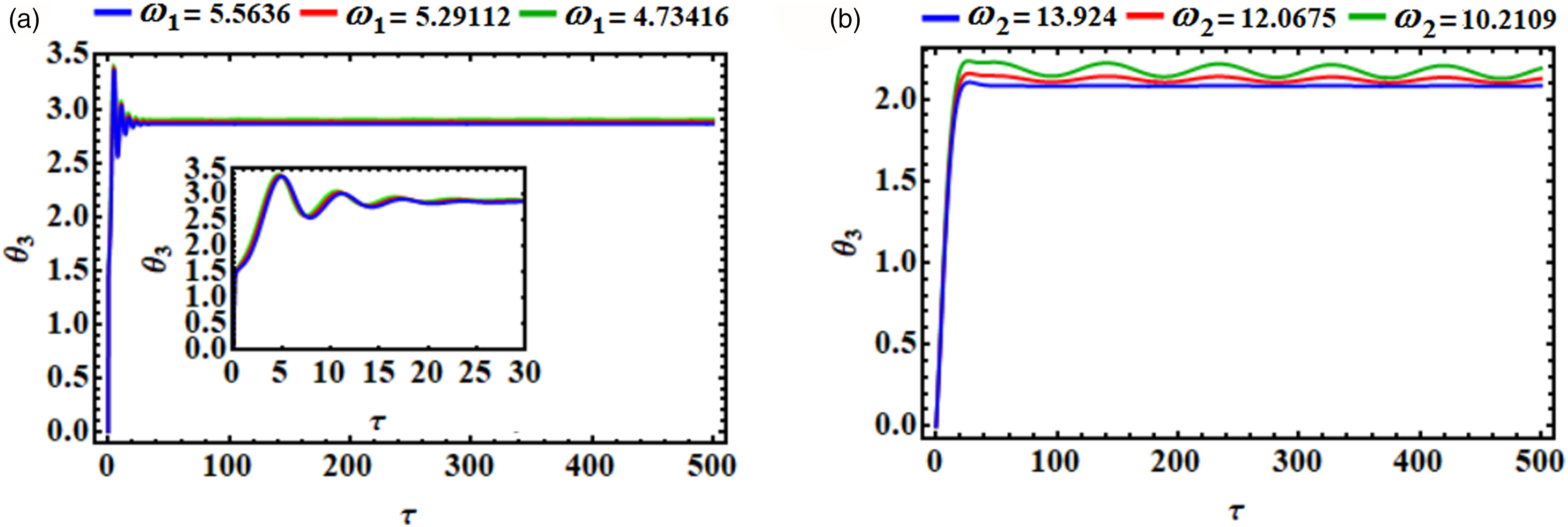
The main purpose of the graphed curves in Figures 6 and 7 is to examine the variation of the third amplitude when and have distinct values. These curves confirmed that the values of the parameters and have no influence on the wave of , as seen in Figures 6(a) and (b). On the contrary, the modified amplitude is impacted with the variation of the values of , as plotted in Figure 6(c). High oscillations are observed at the beginning of time interval when , and then steady behavior is noticed till the end of the time interval. The steady manner begins earlier when the value of increases. Figure 7 investigates the effect of various values of the frequencies and on the temporal course of . Decay waves have been observed with the change of , as indicated in Figure 7(a). In Figure 7(b), the waves rise to a small range and then oscillate periodically till the end of the interval , in which the amplitude of these waves decreases with the increase of values.
Figures 8, 9, 10, 11, 12, and 13 illustrate the time histories of the modified phases and when the influence of the aforementioned parameters is taken into account. It is seen that is impacted by the variation of and , as seen in Figures 8(a) and 9(a), respectively. On the contrary, its behavior has no variation with the change of other parameters, as indicated in Figures 8(a) and (c) and 9(b). In general, the behavior of the explored waves increases with small oscillations during the whole time interval, which was expected from the equations of the system (59).
From the curves of Figures 10 and 11, one can notice that the process of changing the values of and has a positive impact on the plotted waves of . They increase gradually till a specified value and then have a stationary behavior over the entire examined interval, as seen in Figure 10(b), while the waves in Figure 10(c) and 11(a) and (b) increase to a certain value with the increase of time. Moreover, it is seen in Figure 10(a) that has not been impacted by the change in value, which goes back to the structure of the system of equation (59).
The curves of Figures 12 and 13 clearly demonstrate the variation of the function for the above mentioned chosen values of the used parameters and . The oscillated waves in Figure 12(a) and (b) increase during the whole interval and have no variation with the various values of and . On the other hand, positive oscillations are noted, when and have various values, at the beginning of a time interval and then they have steady behavior till the end of this interval, as seen in Figures 12(c) and 13(a), respectively. The influence of values on the plotted waves in Figure 13(b) shows that they are raised until a certain range and then oscillate over the examined interval. According to the aforementioned figures, we can note that the behavior of the plotted waves that describe the modified amplitudes and phases has a stationary form and is free of chaos.
Referring to the plotted curves of the amplitudes and the modified phases one can present the projection of these curves in the planes for the same considered values of the damping and frequency parameters, as seen in Figures 14, 15, 16, 17, 18, and 19. Decay waves are noted for the graphed curves in Figures 14, 15, 16, 17, periodic waves are observed in Figure 18(a) and (b), while spiral curves heading towards one point are drawn in Figures 18(a) and 19. We can say that the difference in the drawn types of curves is due to the complete consistency between the time trajectories of the amplitudes and their corresponding phases. Therefore, the dynamical motion of the system is stable over the studied time interval.
Illustrates the phase plane at and for various values of: (a) , (b) , and (c) .
Shows the phase plane at and for various values of: (a) , and (b) .
Shows the phase plane at and for various values of: (a) , (b) , and (c) .
Presents the phase plane at and for various values of: (a) , and (b) .
Presents the phase plane at and for various values of: (a) , (b) , and (c) .
Illustrates the phase plane at and for various values of: (a) , and (b) .
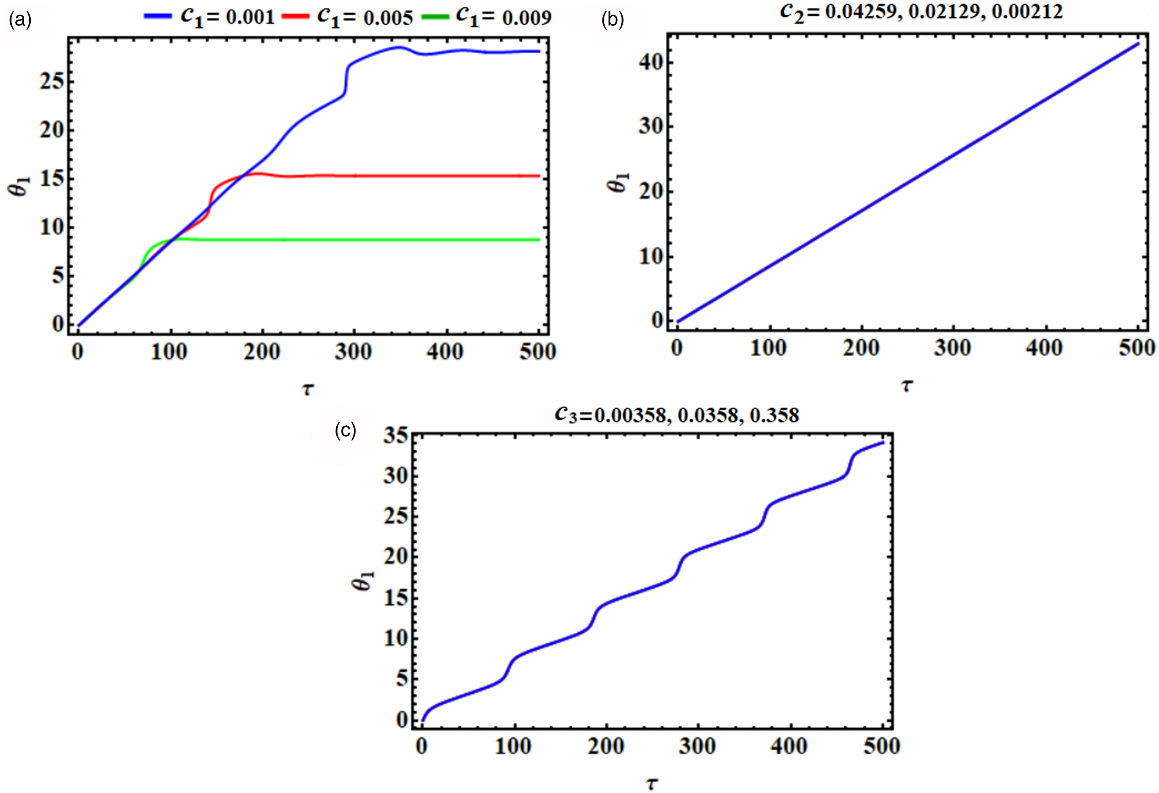
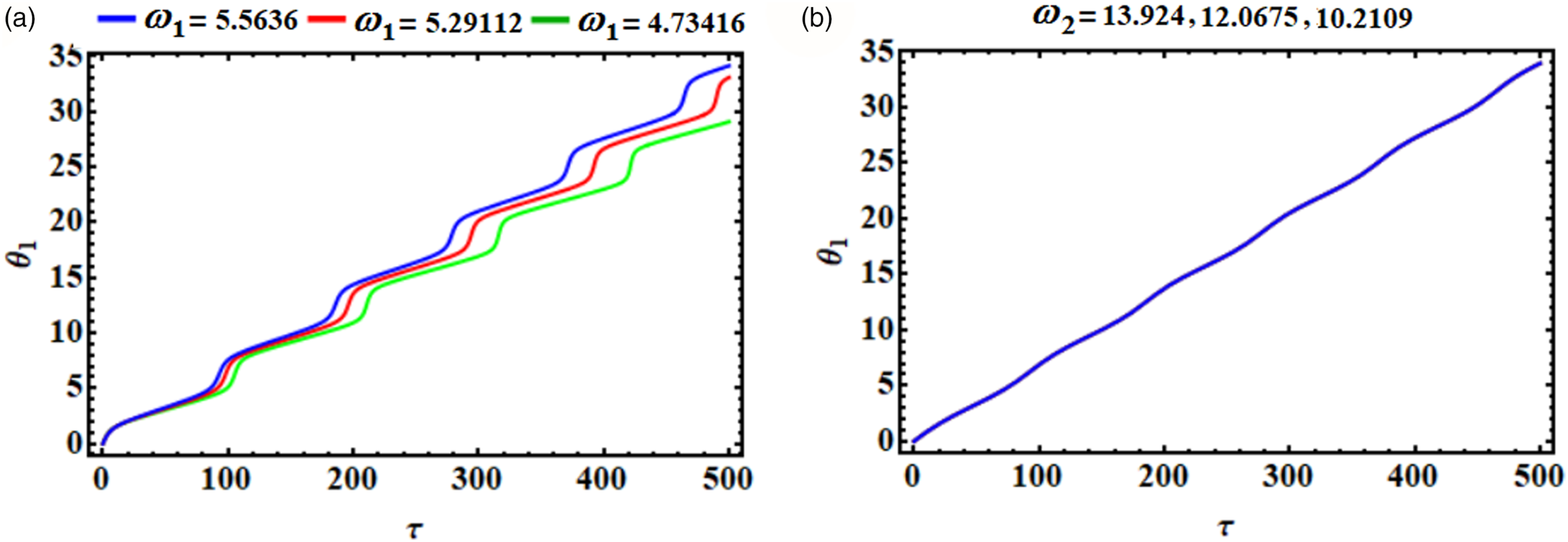
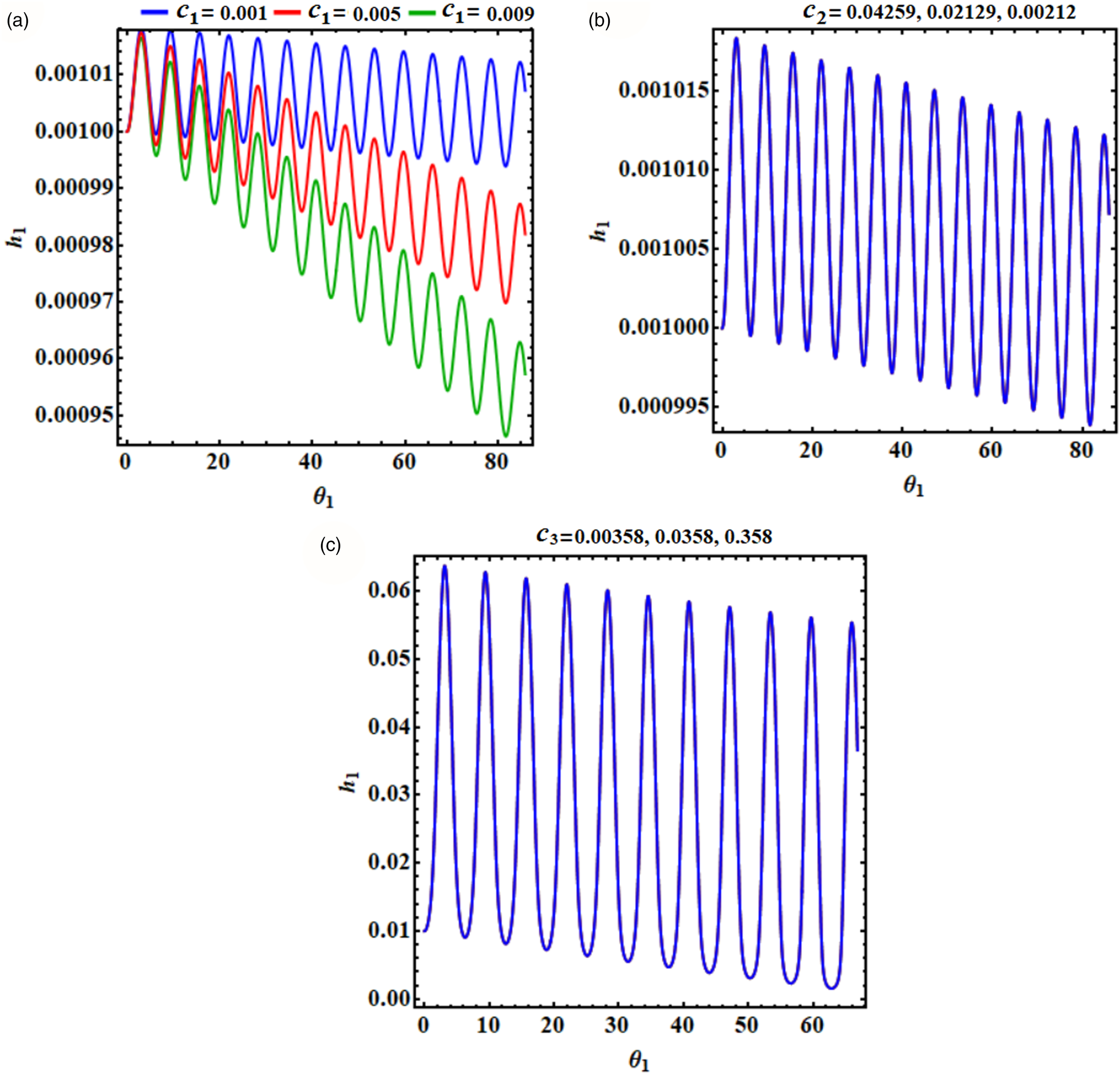
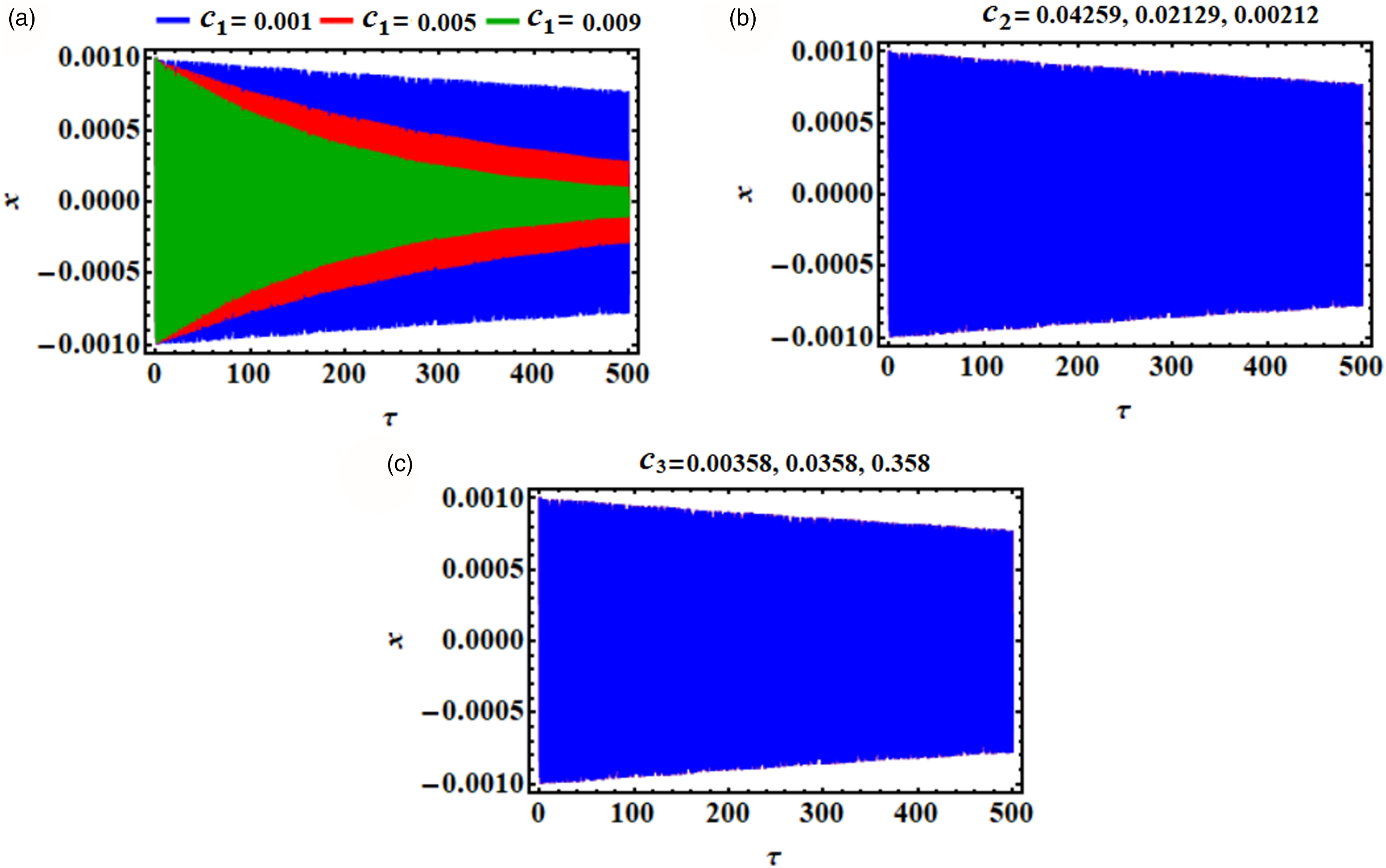
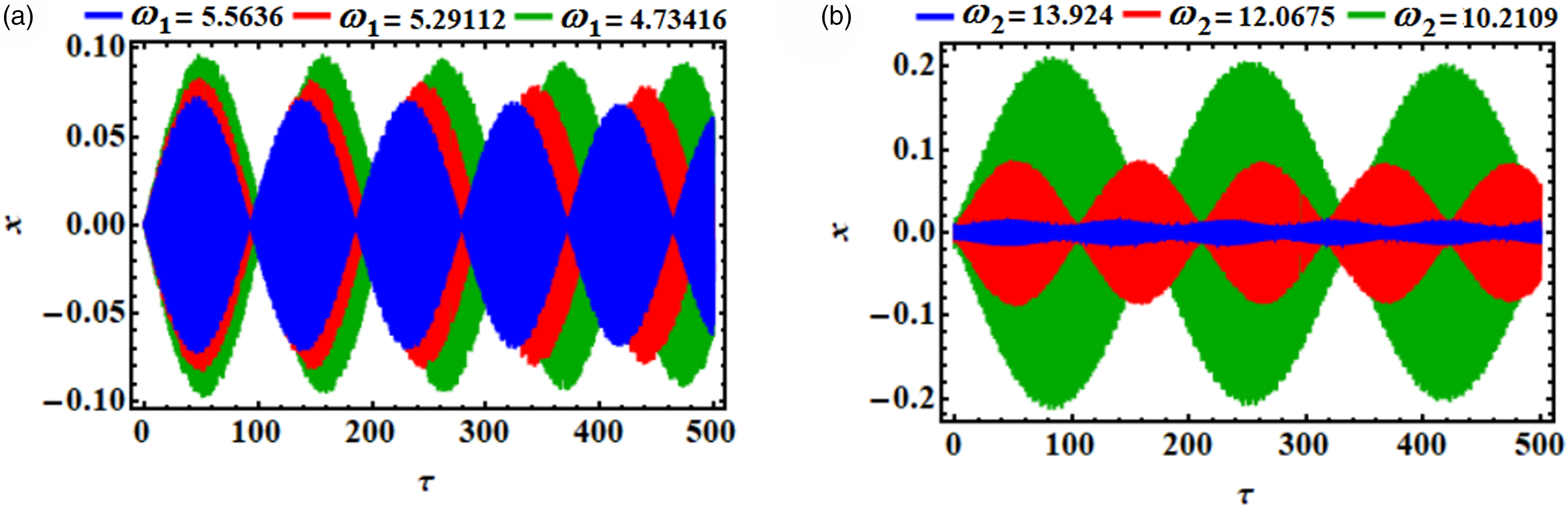
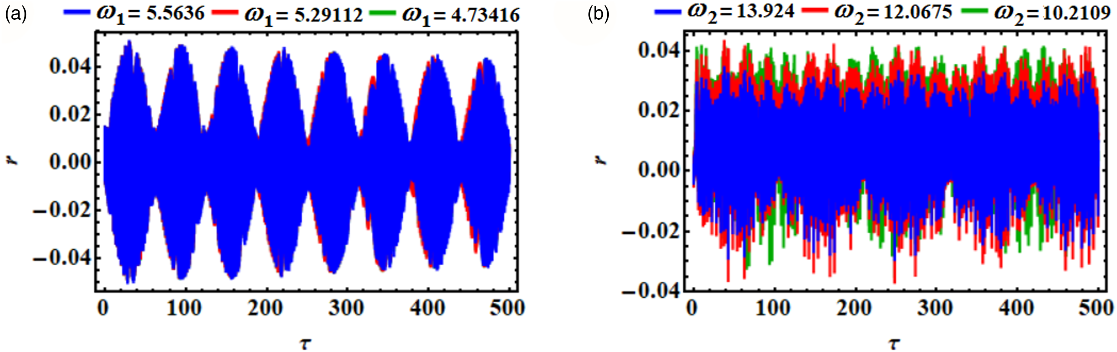
The main purpose of the explored curves in Figures 20, 21, 22, 23, 24, 25 is to investigate the time histories of the achieved asymptotic solutions and , taking into account the above-selected values of the parameters and . Decay waves are plotted in parts of Figure 20, in which the solution is impacted by the values of and the amplitude of the graphed waves decreases with the increase of values, as demonstrated in part (a). On the other side, this solution isn’t influenced by the selected values of and , as indicated in the other parts (b) and (c). Periodic waves describing the temporal behavior of this solution are graphed in Figures 21(a) and (b) when and have the same considered values above, in which their amplitudes increase with the decrease of and values. According to this simulation, one concludes that the plotted wave of the solution is stable during the whole-time interval.
Reveals the solution at and for various values of: (a) , (b) , and (c) .
Shows the solution at and for various values of: (a) , and (b) .
The behavior of at and for various values of: (a) , (b) , and (c) .
The behavior of at and for various values of: (a) , and (b) .
The behavior of at and for various values of: (a) , (b) ,and (c) .
The behavior of at and for various values of: (a) , and (b) .
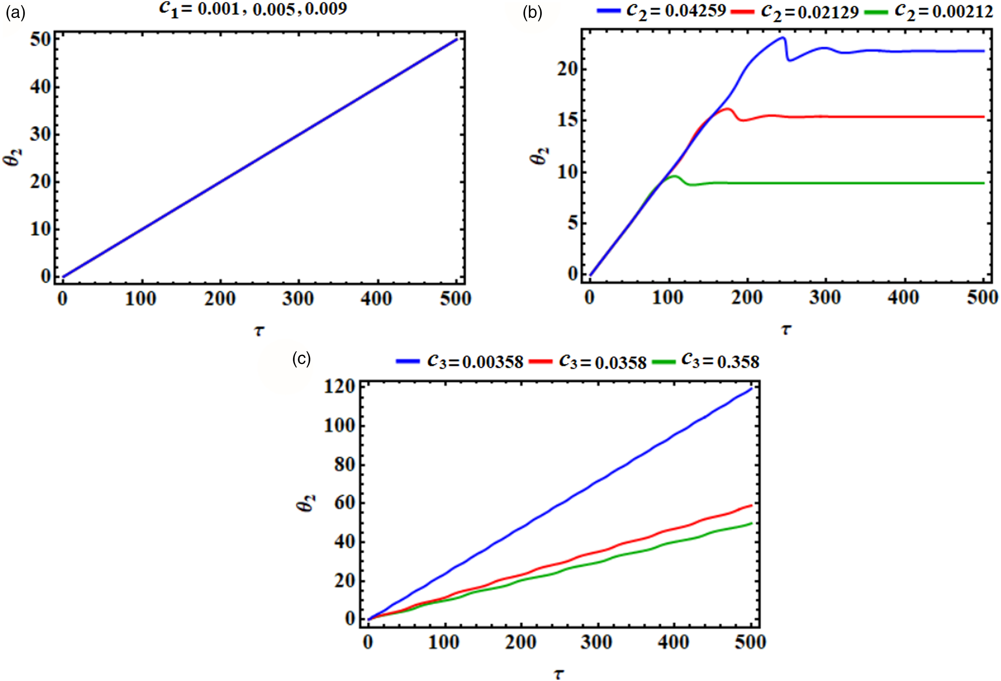
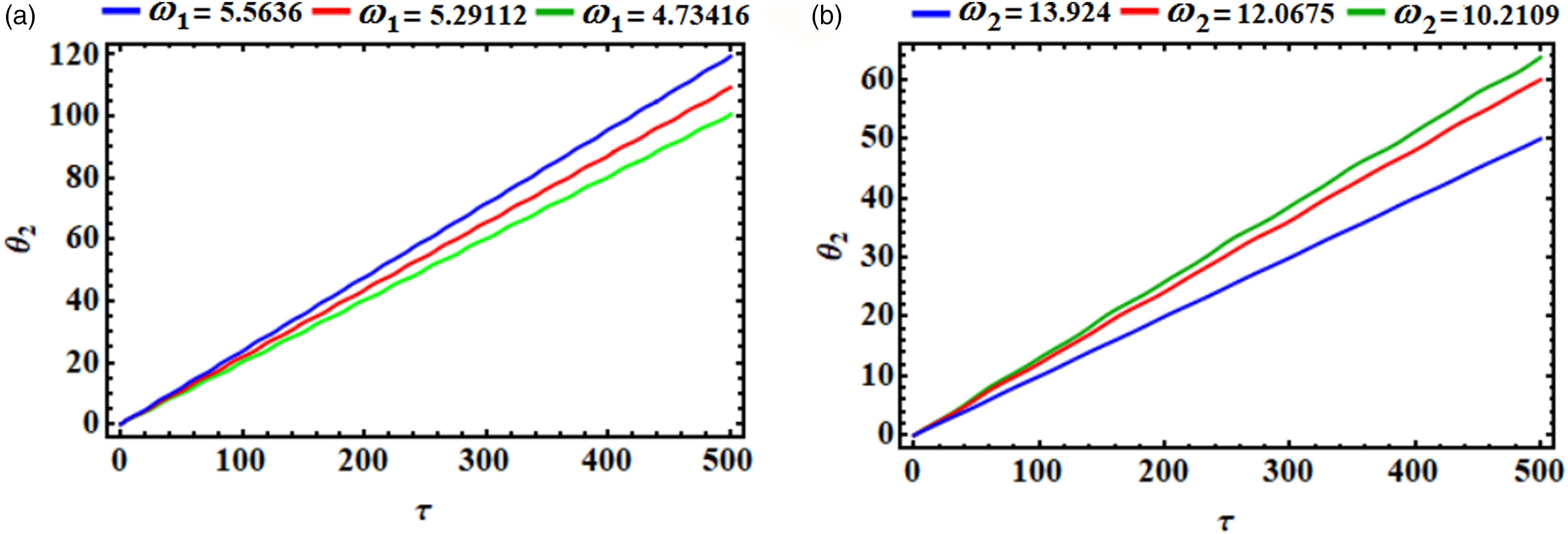
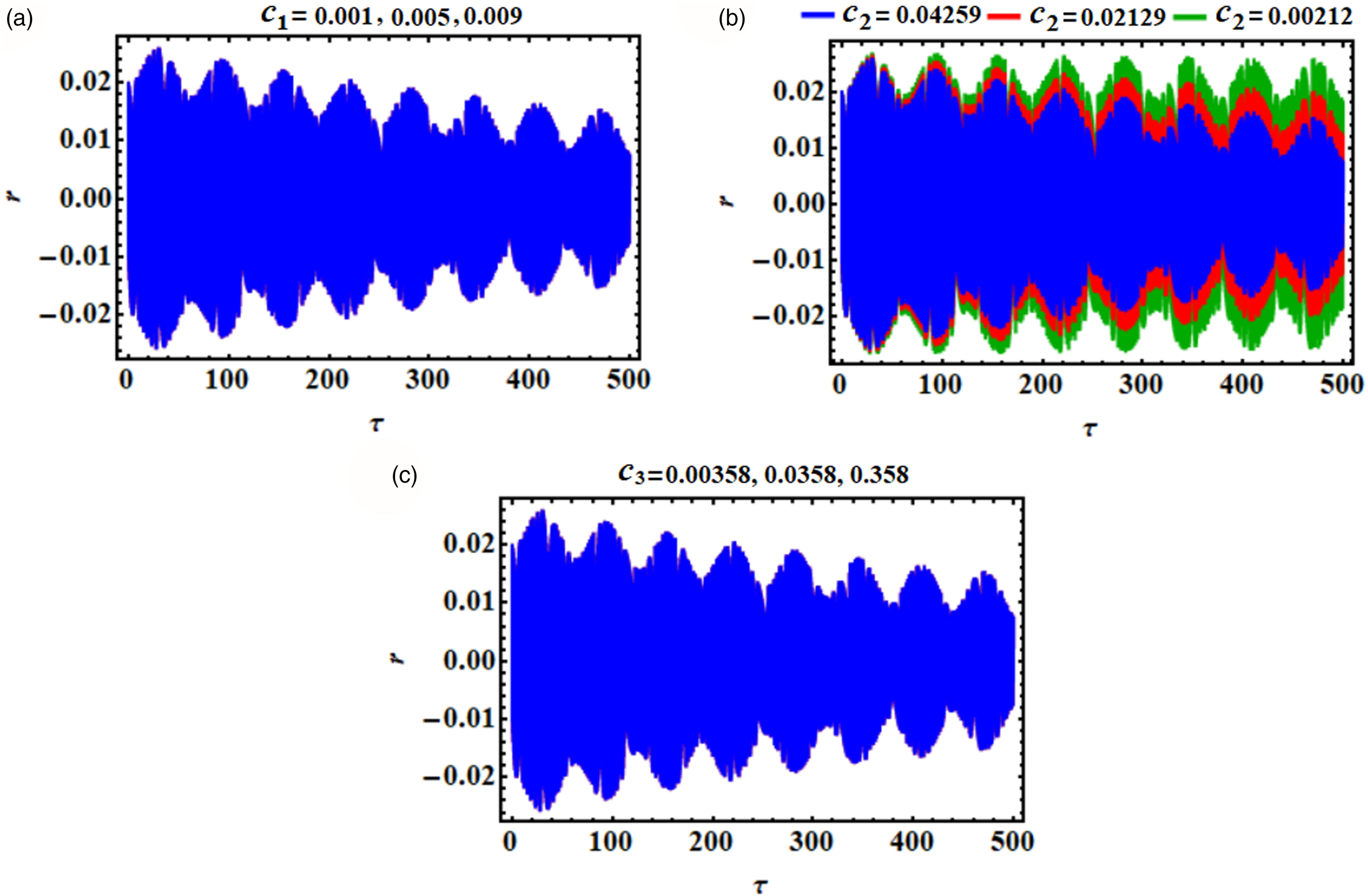
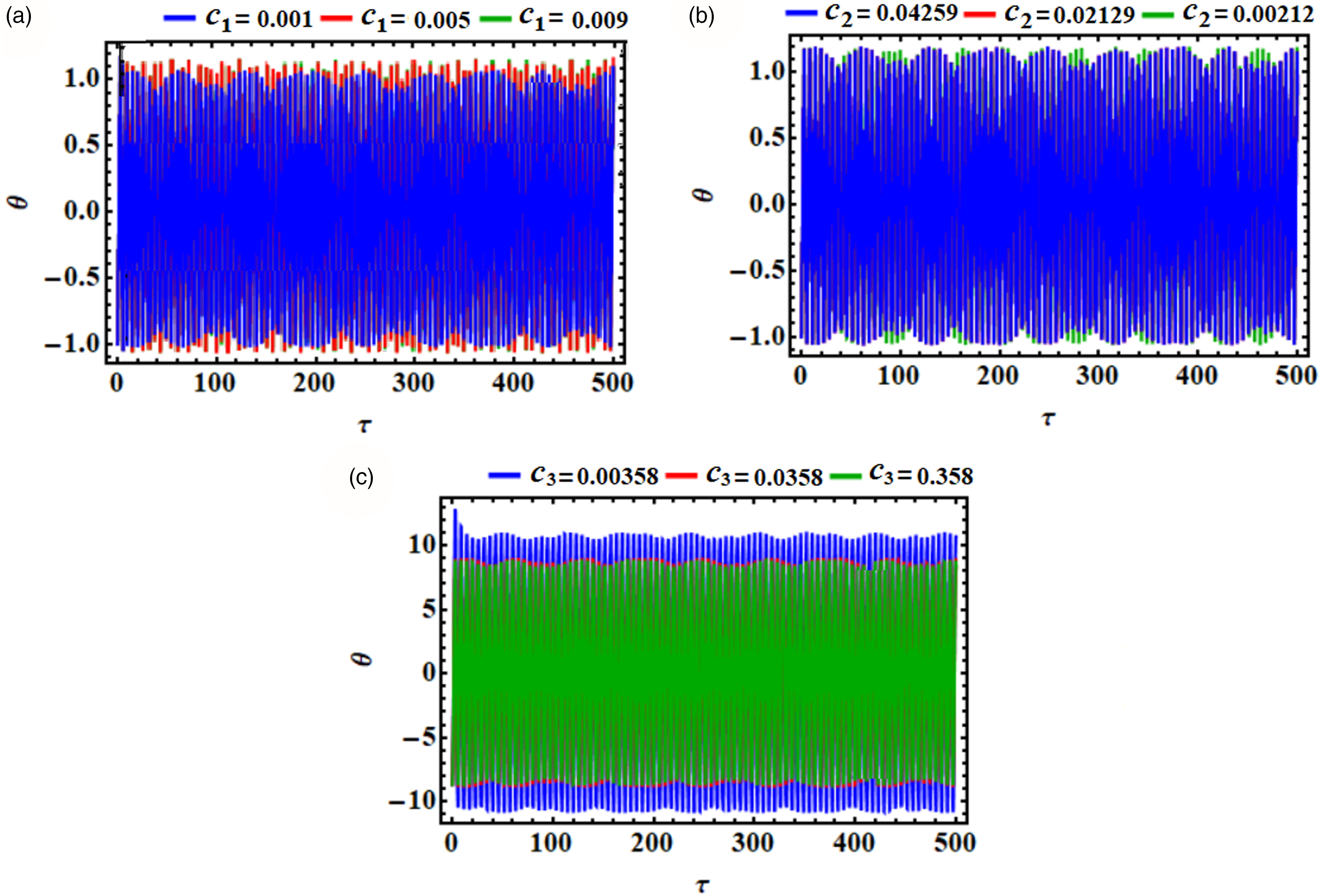
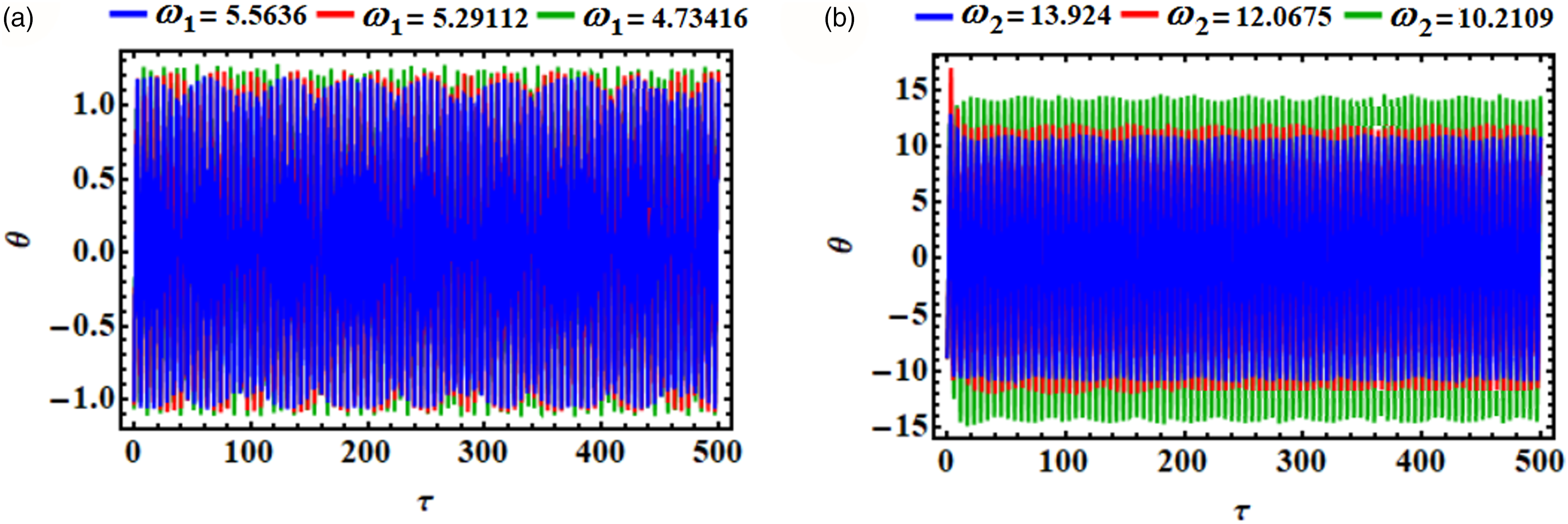
The variation of the solution via the dimensionless time is graphed, respectively, in Figures 22 and 23 for various values of the damping and frequency parameters. The plotted waves behave in the form of decay wave packets, in which this solution is acted only by the values of . The decay reaches its maximum behavior when the damping value is high, as seen in parts of Figure 22. Periodic and quasi-periodic waves with a slight decay for the function are graphed, respectively, in parts (a) and (b) of Figure 23. The wave’s amplitude decreases with the increase in values.
The time history of the asymptotic solution is drawn in Figures 24 and 25, when the damping parameters and frequency ones have various values. The drawn curves have stationary behavior over the examined interval of time, as seen in parts of these figures.
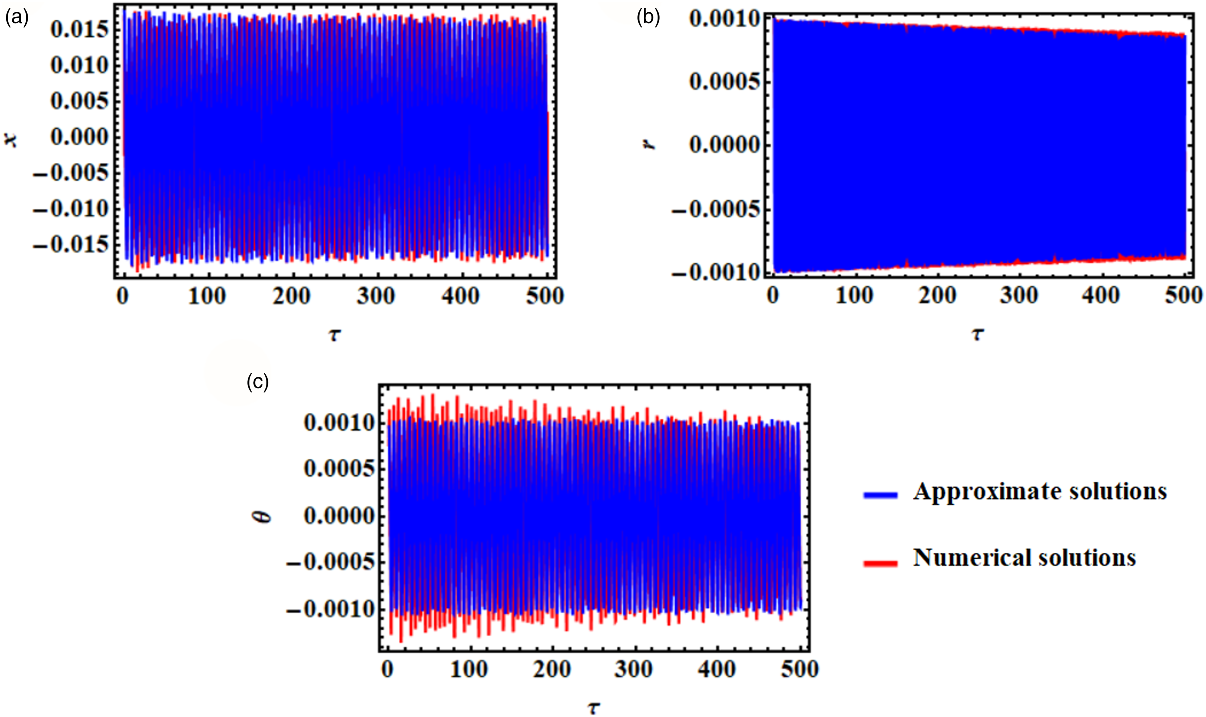
Figure 26 shows the time histories of both the achieved approximate and the numerical solutions over the interval . The represented waves of both solutions have periodic or quasi-periodic forms with little decay, which gives an induction about the stability of these waves. A closer look at this figure shows that there is a great deal of consistency between these solutions, which supports the importance of the used perturbation approach that produces accurate approximate solutions that are compatible with the numerical solutions of the original governing system.
Describes the time history for both the numerical and approximate solutions.
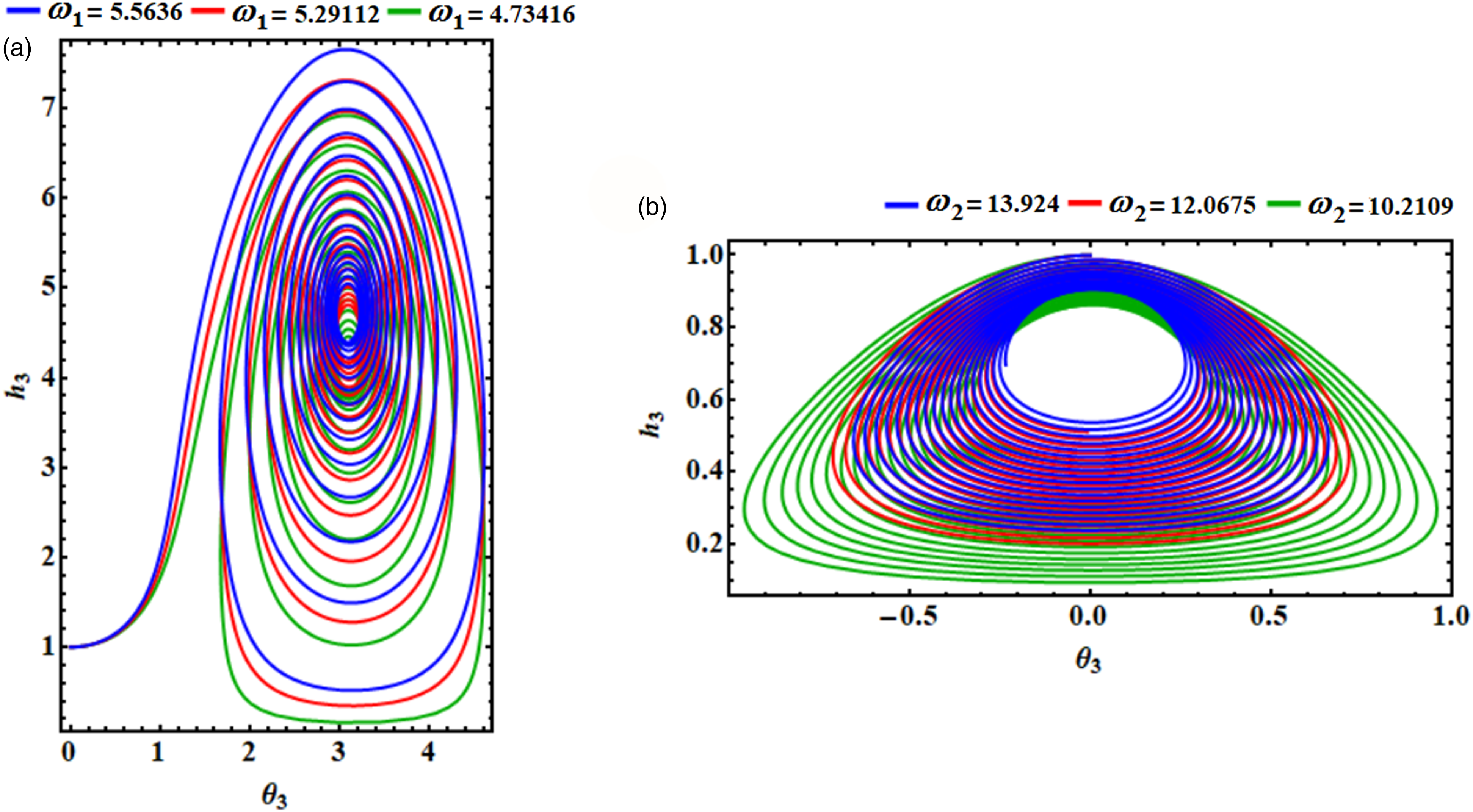
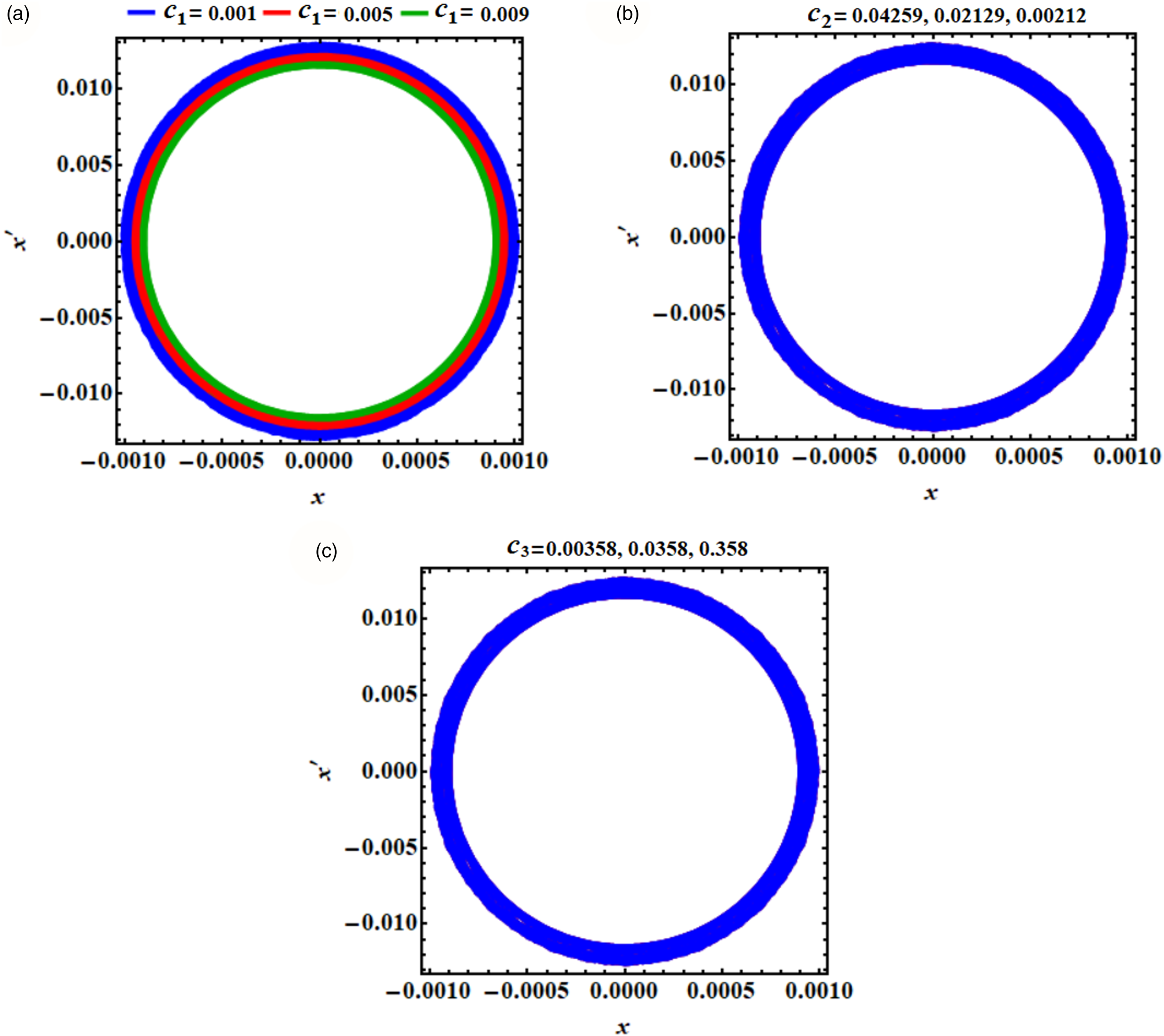
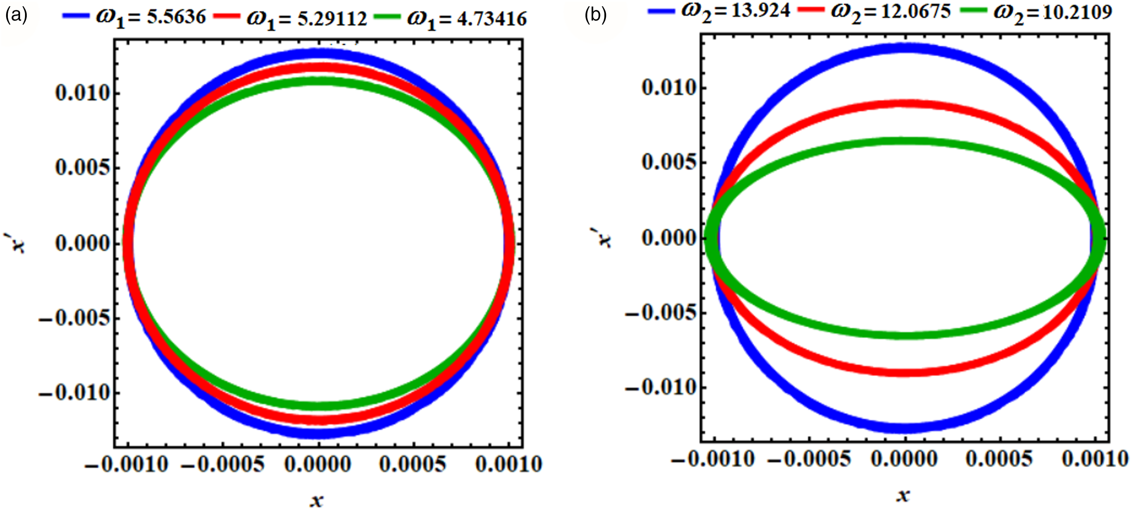
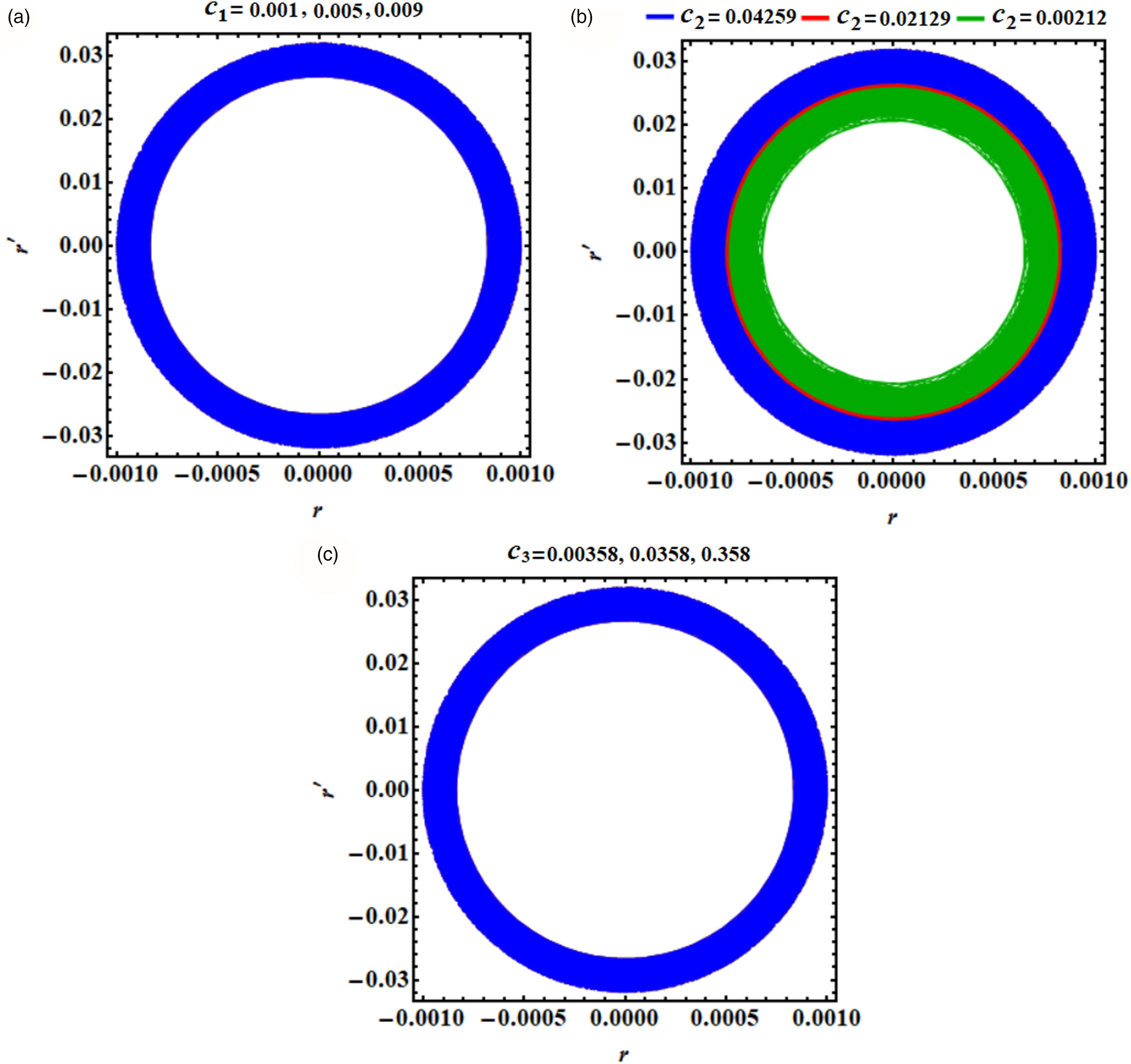
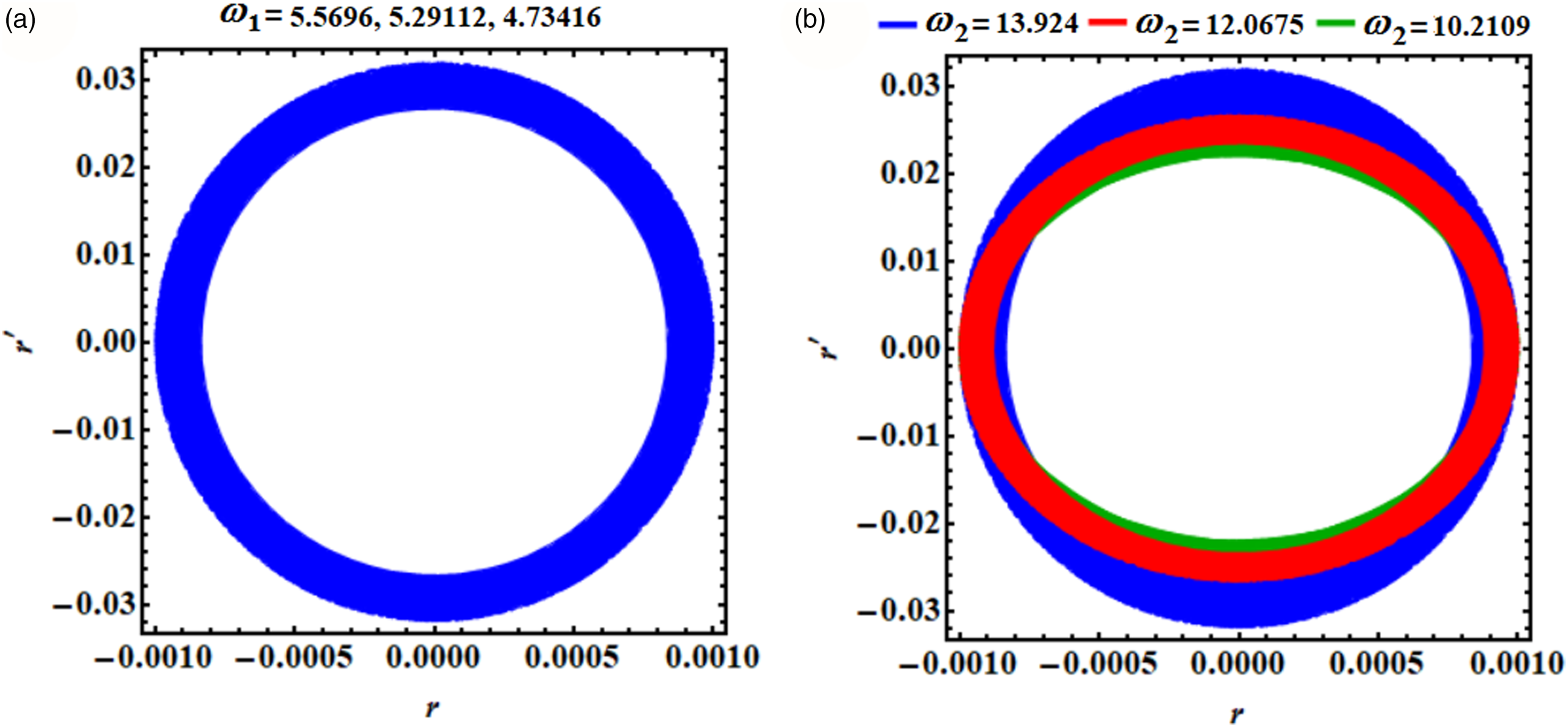
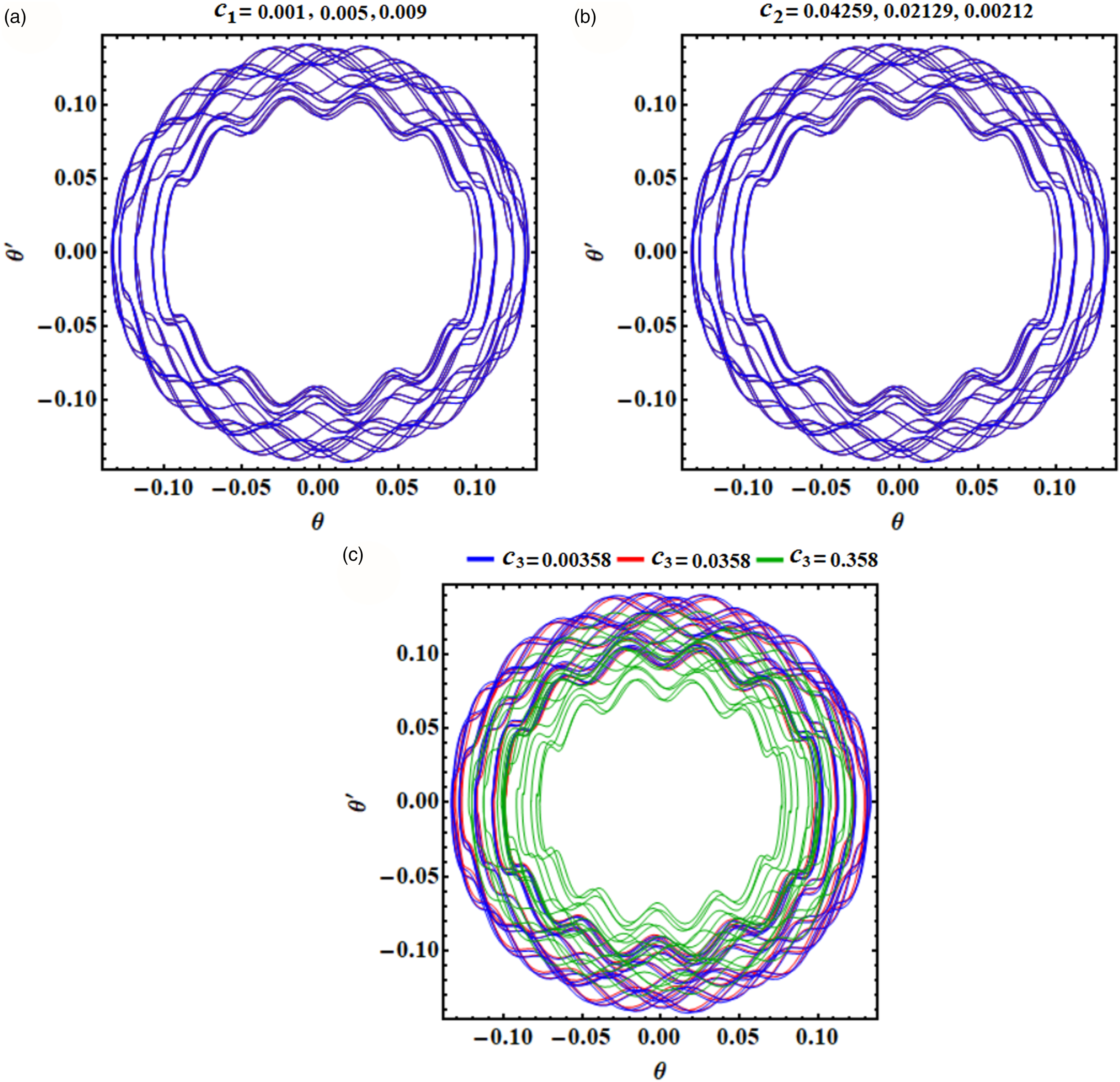
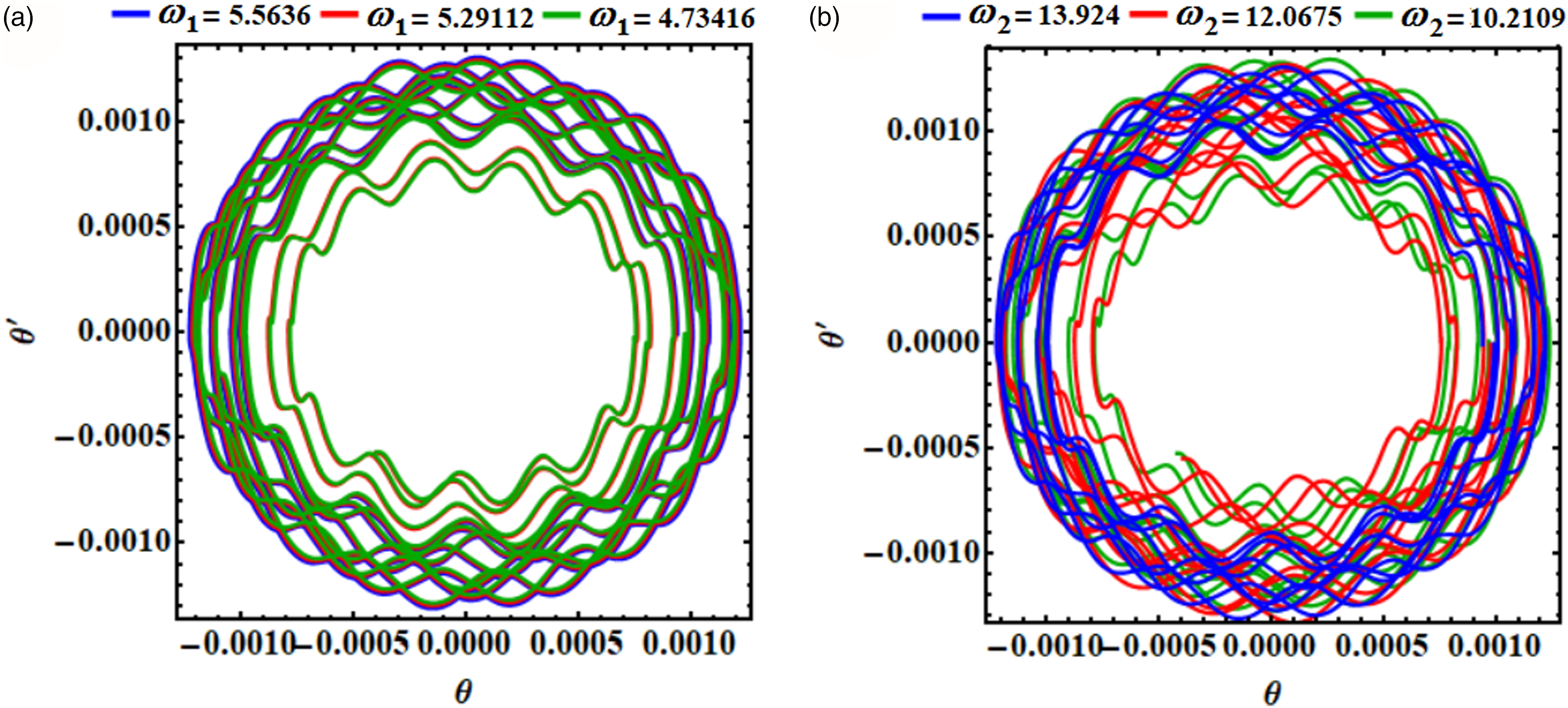
The phase portraits curves for the obtained solutions and are depicted in Figures 27, 28, 29, 30, 31 and 32. These curves are drawn for the same values of and to show closed curves whether symmetric or not that gives an induction about the stationary behavior of the obtained solutions. It is noticed that the phase portraits of the solution have deformation closed curves when and have different values. This deformation is due to that the equation of the first approximation of this solution is nonhomogeneous.
Illustrates the phase portraits for the solution when and for: (a) , (b) , and (c) .
Illustrates the phase portraits for the solution at and for: (a) , and (b) .
Describes the phase portraits for the solution at and for: (a) , (b) , and (c) .
Illustrates the phase portraits for the solution at and for: (a) , and (b) .
Presents the phase portraits for the solution at and for: (a) , (b) , and (c) .
Illustrates the phase portraits for the solution at and for: (a) , and (b) .
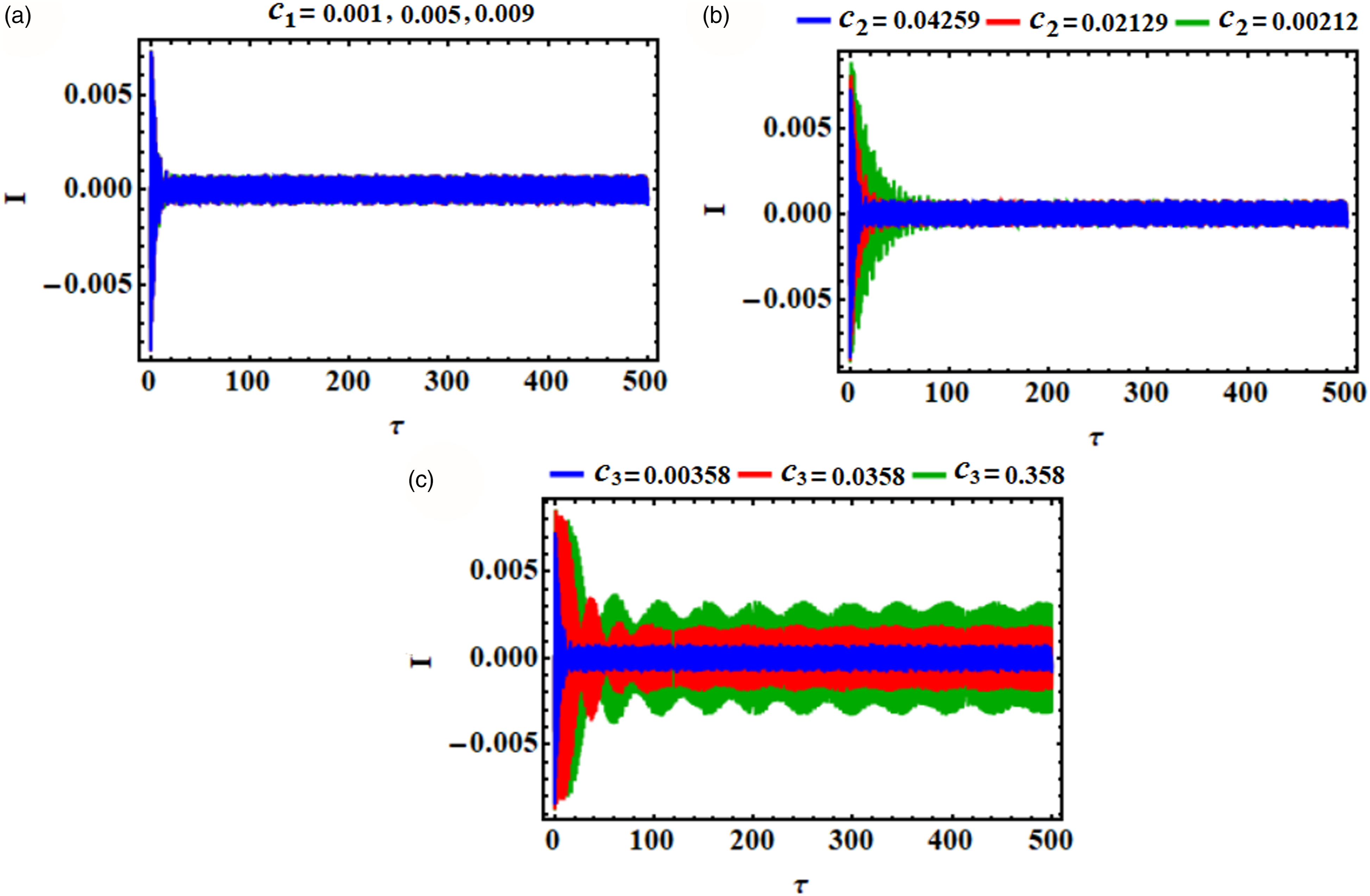
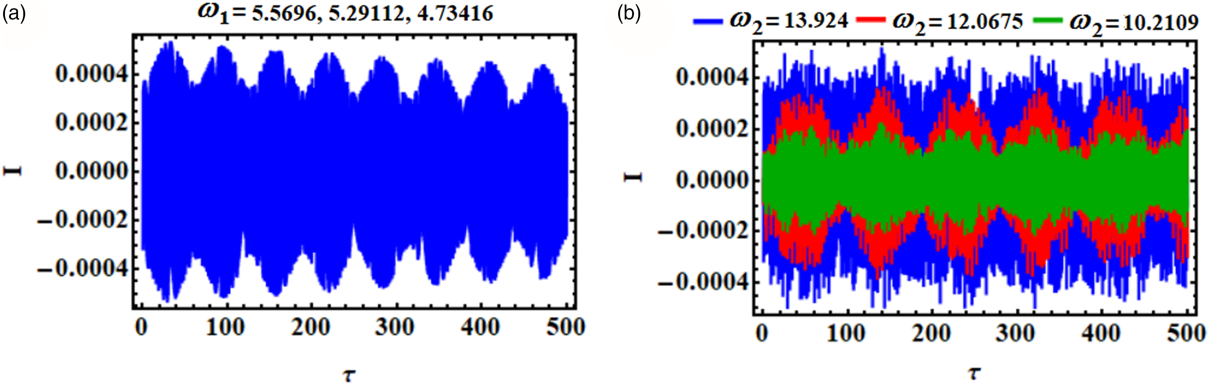
Curves of the generated current by the EH device are represented graphically in Figures 33 and 34 for various values of the aforementioned parameters of damping and frequency. These curves have been graphed according to the current equation (5) to show their time behavior over the examined interval. Small amplitudes of the produced current are noted, resulting in low power levels (in milliwatts) at the output, which is considered suitable for sensor applications. The waveform of the current exhibits the existence of harmonic signals on the basic ones at the beginning of the wave's transient current caused by the RL circuit. The current then exhibits stationary behavior, which is necessary for usage. It is clear that the current has not been impacted by the change in , as seen in Figure 33(a), while it has been influenced by the values of and , as indicated in Figures 33(b) and (c). Based on the drawn curves, the current rises and oscillates at the beginning of the time interval until a certain time value, and then it has steady behavior. Increasing the value of the damping coefficient leads to faster wave stability than its lower value.
Detects the time history of the current at and for various values of: (a) , (b) , and (c) .
Detects the time history of the current at and for various values of: (a) , and (b) .
The good effect of changing the frequency values is clearly evident in Figure 34, in which periodic waves are graphed with a slight decay at the end of the time interval, and we find that this change seams slightly and clearly when and vary.
Steady-State solutions
The purpose of the present section is to investigate the model's vibrations in the steady-state scenario. In other words, when the transient process's vibrations disappear due to the presence of the system's damping. In these circumstances, the system of ME (59) plays a crucial role in defining this goal, in which the amplitudes and the adjusted phases have zero first derivatives. As a result, one can write
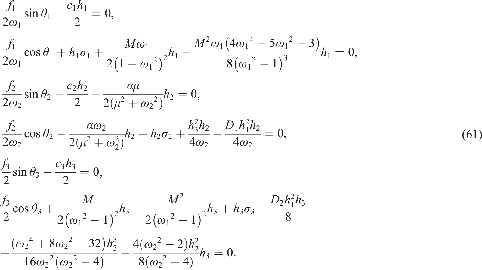
According to the above conditions, equations of system (59) have the form
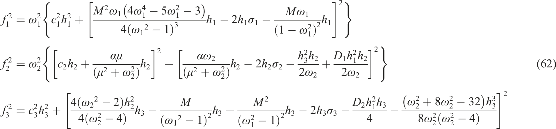
After we get rid of the modified phases from equation (61), we can obtain the following nonlinear equations in terms of and
The oscillations in the steady-state scenario are regarded as crucial aspects for the stability analysis of the system of ME. We take into account the system's performance in an area that is relatively near the fixed locations to accomplish such a scenario. Consequently, the below expressions of and are taken into consideration
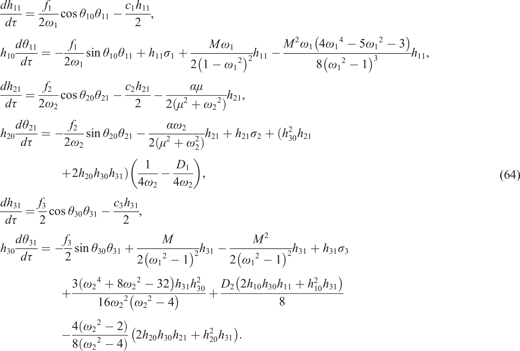
where and are the unperturbed steady-state solutions, while and are the suggested perturbed ones. The substitution of (63) into (59) yields
As mentioned above and refer to the un-identified functions. Then, we can express their solutions as a linear superposition of , where and are constants and eigenvalues, respectively. If and of the steady-state solution are stable, then the real parts of the roots of the next characteristic equation of (64) will be negative
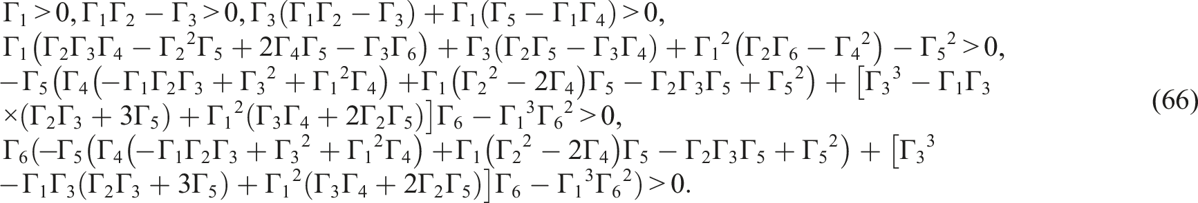
Based on the criteria of Routh–Hurwitz,40 the stability’s conditions of can be written in the following forms
The analysis of stability
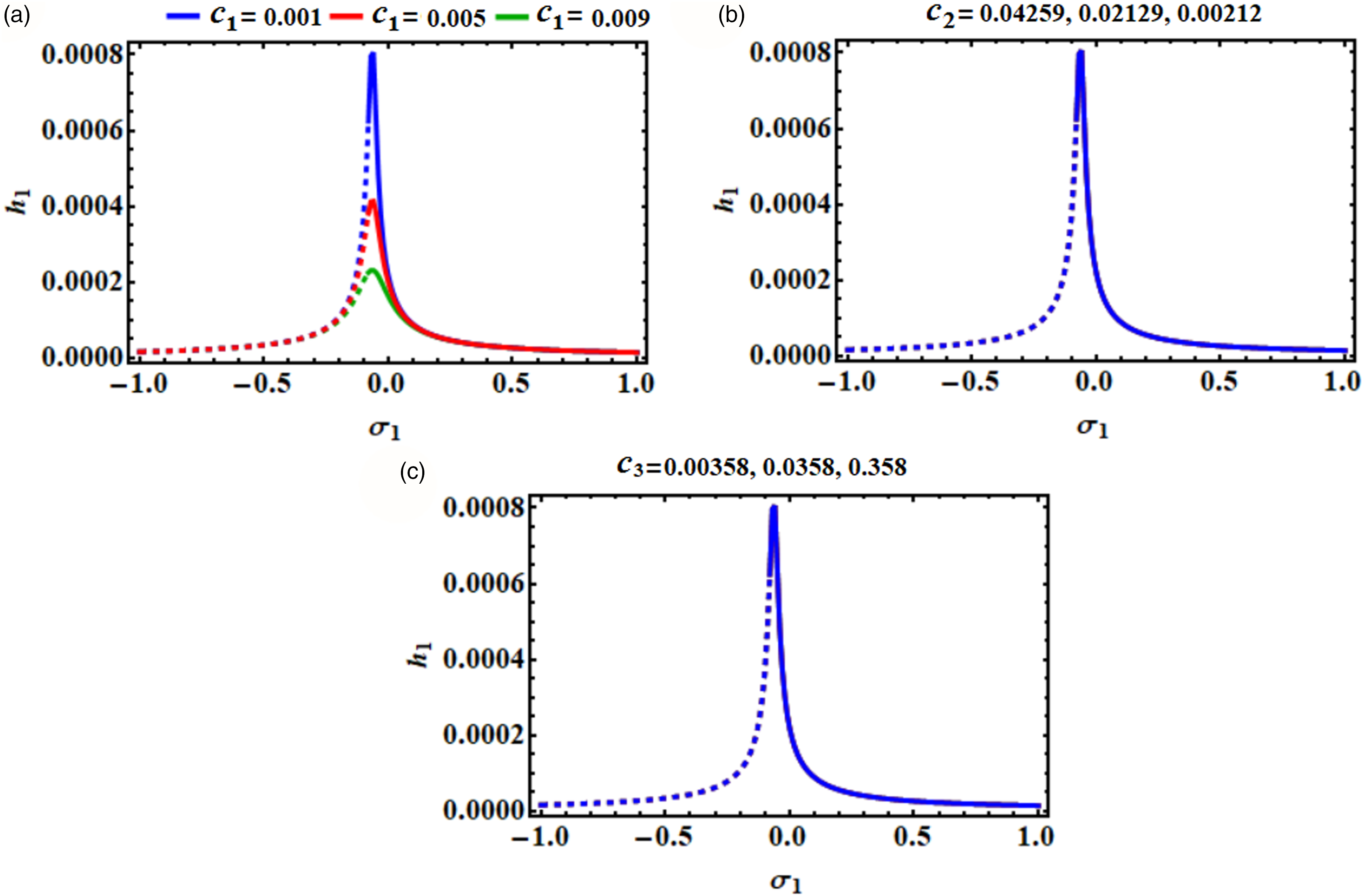
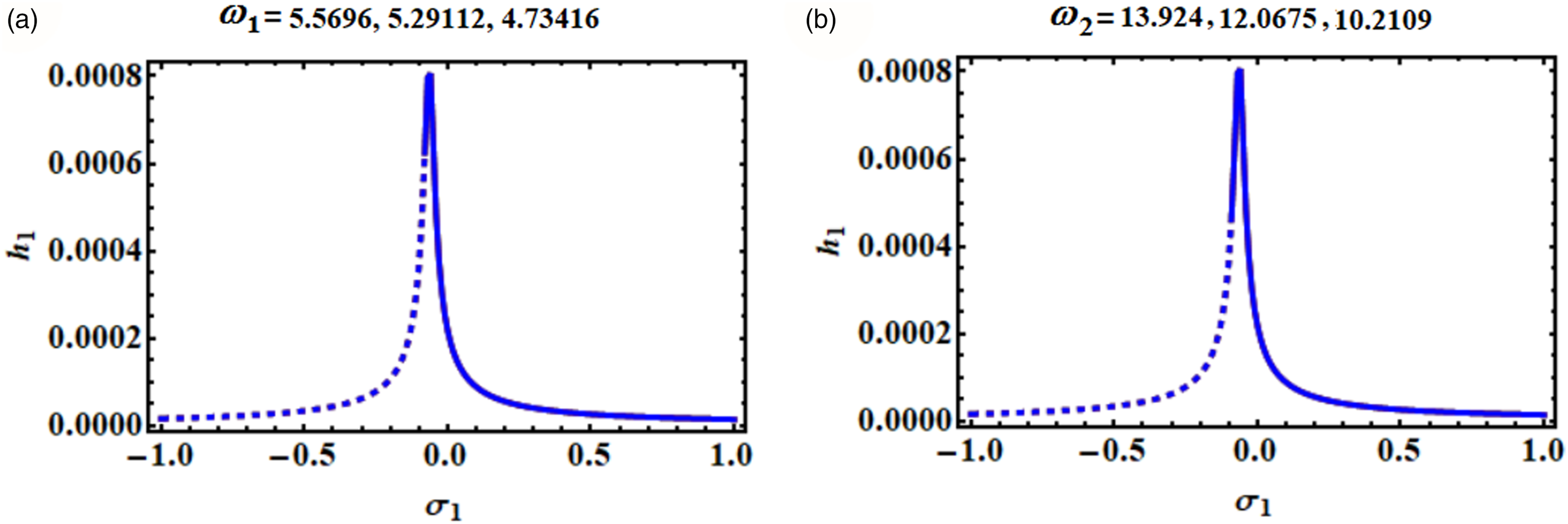
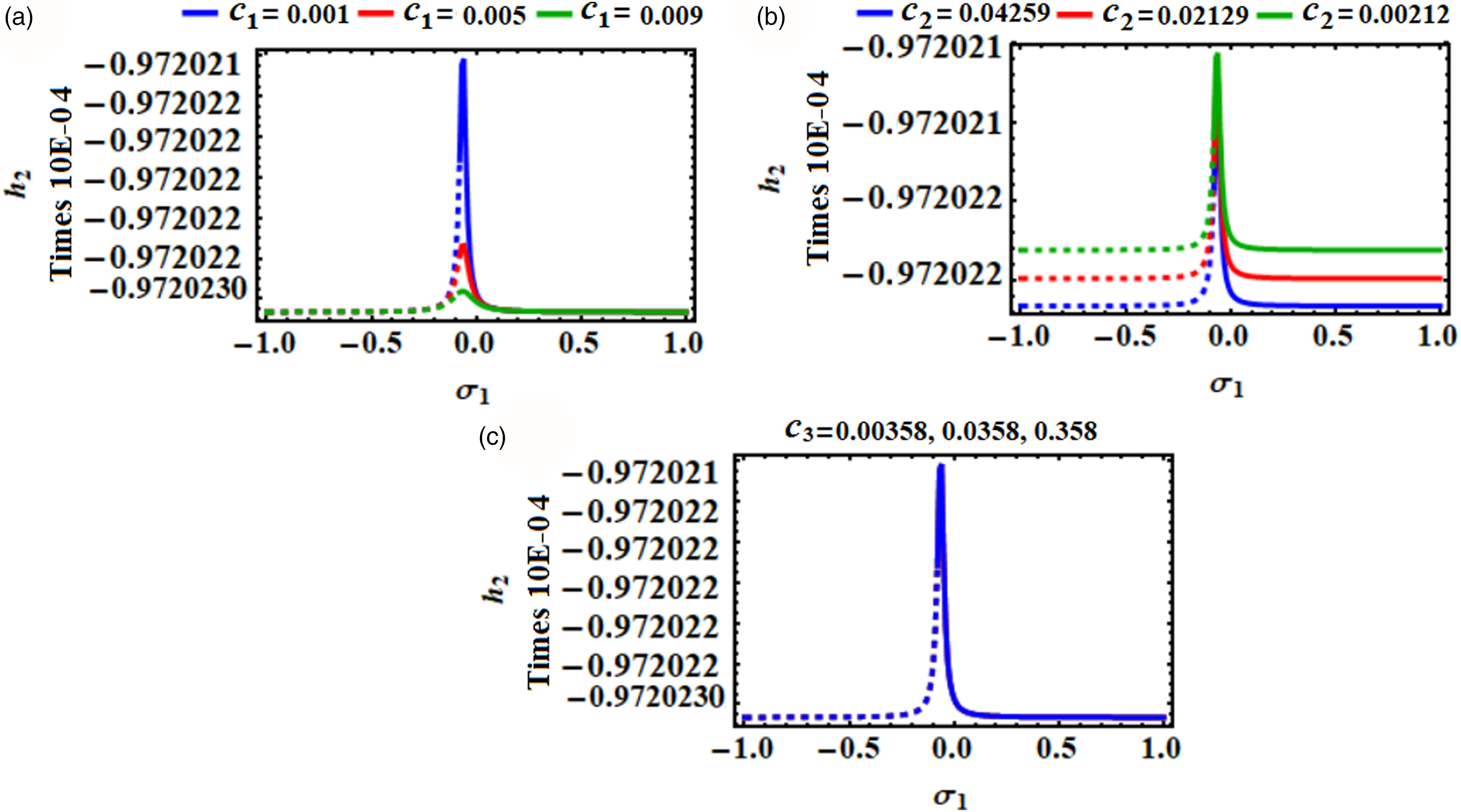
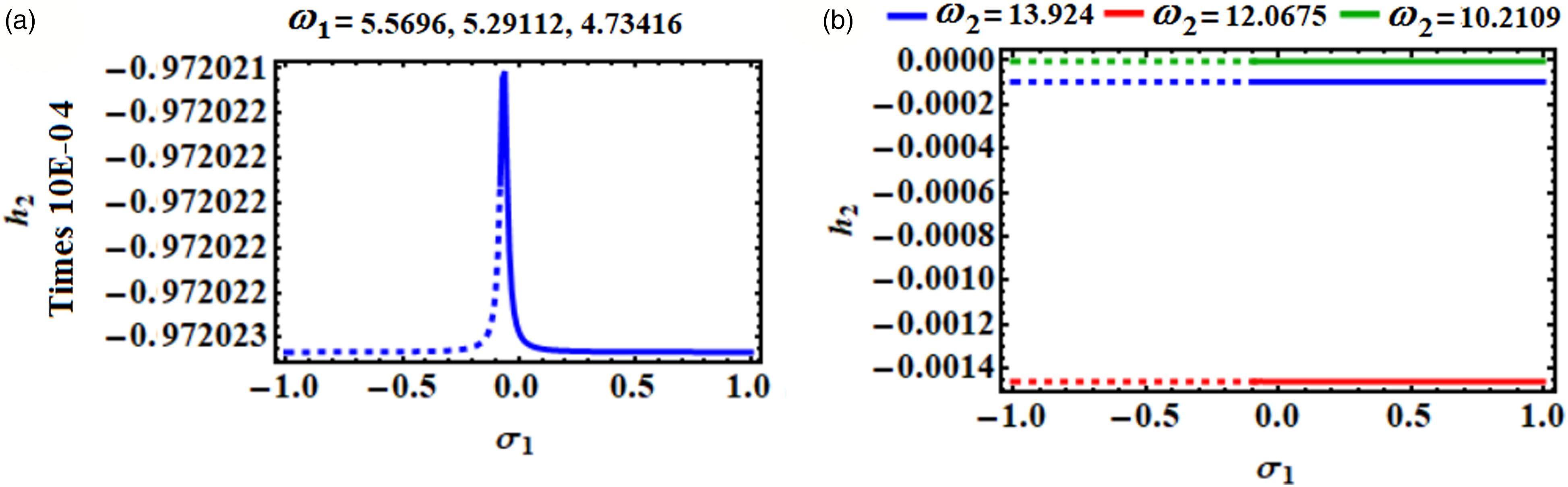
The topic of studying the stability of steady-state oscillations is especially important and unique. Therefore, the stability of the considered system is checked in the current section using the approach of nonlinear stability analysis, in which the stability simulation and the influence of the acted parameters are evaluated. It is noted that some important parameters like; the frequencies , detuning parameters , and damping coefficients , play a significant role in the processes of stability. A specific action was used with different system parameters to produce the stability diagrams for the system of ME (59). For various parametrical zones, the altered amplitudes fluctuation with time are depicted, and their characteristics are shown throughout phase plane paths. The possible fixed points of the system are drawn. In Figures 35, 36, 37, 38, 39, and 40, the change of the potential fixed points with various detuning parameters is examined, in which its range is considered to be . The dotted curve refers to the unstable range, on the contrast the continuous lines denote the stable one. Figures 35 and 36 show the variation of via when the used different values of and are considered, respectively. One can see from the drawn frequency response curves (FRC) in Figures 35, 37, and 39 that the ranges of the unstable and stable fixed points are, respectively, and when have the considered various values. On the other hand, the fixed point reverses its stability at . Figures 36, 38, 39, and 40 show the influence of , on the plotted stability curves in the plane .It is found that the fixed point reverses its stability at and at the considered values of and respectively.
Shows the FRC in the plane at and when: (a) , (b) , and (c) .
Explains the FRC in the plane at and when: (a) , and (b) .
Investigates the FRC in the plane at and when: (a) , (b) , and (c) .
Shows the FRC in the plane at and when: (a) , and (b) .
Presents stability and instability ranges in the plane at and when: (a) , (b) , and (c) .
Presents stability and instability ranges in the plane at and when: (a) , and (b) .
Based on the above simulation, the examined system has one critical fixed point for all values , which means that it is under the influence of transcritical bifurcation. This demonstrates that there is no pattern of system behavior that is qualitative when the parameters are changed.
Conclusion
The motion of a 3DOF dynamical system composed of two coupled parts, which are a dynamic part and a HE device, has been studied. The magnet oscillating in the coil of this device determines how the system is constructed. The electromotive force produced an electric potential, which has been used to harvest the energy. The EOM of this system have been derived using LE and solved analytically up to a third-order using the MSM. The obtained novel solutions have been validated through comparison with the numerical solutions of the EOM, which demonstrate a high level of consistency. Three basic cases of external resonance have been simultaneously explored to determine the solvability conditions and the ME. To illustrate their behaviors at any given time, specific diagrams of time histories have been drawn and discussed for the obtained solutions and the current, taking into account certain values of the used parameters. The system of ME has been solved numerically to reveal the amplitudes and adjusted phases for the same data of the considered parameters. The stability criteria of Routh–Hurwitz have been used to discuss the stability and instability zones of this system and show the influence of the acting parameters on the FRC. Therefore, it is possible to convert vibrational motion into electrical energy by including an energy harvester in vibrating dynamical systems. This electrical energy can then be used for a variety of daily tasks, such as remote medical sensing, environmental and structural monitoring, concrete pouring, military applications, and space exploration.
Supplemental Material
Supplemental Material - On the influence of an energy harvesting device on a dynamical system
Supplemental Material for On the influence of an energy harvesting device on a dynamical system by TS Amer, A Arab and AA Galal in Journal of Low Frequency Noise, Vibration & Active Control
Footnotes
Authors statements
TS Amer: Supervision, Investigation, Methodology, Data curation, Conceptualization, Validation, Reviewing and Editing.
A Arab: Resources, Methodology, Conceptualization, Data curation, Validation, Writing- Original draft preparation.
AA Galal: Supervision, Conceptualization, Resources, Formal analysis, Validation, Writing- Original draft preparation, Visualization and Reviewing.
Declaration of conflicting interests
The author(s) declared no potential conflicts of interest with respect to the research, authorship, and/or publication of this article.
Funding
The author(s) received no financial support for the research, authorship, and/or publication of this article.
ORCID iDs
TS Amer
AA Galal
Supplemental Material
Supplemental material for this article is available online.
References
1.
ParadisoJAStarnerT. Energy scavenging for mobile and wireless electronics. IEEE Pervasive Computing2005; 4(1): 18–27.
2.
MizunoMChetwyndDG. Investigation of a resonance microgenerator. J Micromech Microeng2003; 13(2): 209–216.
3.
MitchesonPDYeatmanEMRaoGK, et al.Energy harvesting from human and machine motion for wireless electronic devices. Proc IEEE2008; 96(9): 1457–1486.
4.
NaruseYMatsubaraNMabuchiK, et al.Electrostatic micro power generation from low-frequency vibration such as human motion. J Micromech Microeng2009; 19(9): 094002.
5.
TsutsuminoTSuzukiYKasagiN, et al.Seismic power generator using high performance polymer electrets. In: Proc of IEEE MEMS Istanbul, Turkey, 2006, pp. 98–101.
6.
SuzukiYEdamotoMKasagiN, et al.Micro electret energy harvesting device with analogue impedance conversion circuit. Proc Power MEMS2008; 8: 7–10.
7.
GuL. Low-frequency piezoelectric energy harvesting prototype suitable for the MEMS implementation. Microelectro J2011; 42: 277–282.
8.
GalchevTAktakkaEEKimH, et al.A piezoelectric frequency-increased power generator for scavenging low-frequency ambient vibration. Proc Of MEMS Hong Kong2010: 1203–1206.
9.
NguyenHTGenovDABardaweelH. Vibration energy harvesting using magnetic spring based nonlinear oscillators: Design strategies and insights. Appl Energy2020; 269: 115102.
10.
NiaEMZawawiNAWASinghSM. A review of walking energy harvesting using piezoelectric materials. IOP Conf Series, Mater Sci Eng2017; 291(1): 012026.
11.
JiangWHanXChenL, et al.Improving energy harvesting by internal resonance in a spring-pendulum system, Acta Mech Sin36, 618-623 (2020).
12.
TranNGhayeshMHArjomandiM. Ambient vibration energy harvesters: a review on non-linear techniques for performance enhancement. Int J Eng Sci2018; 127: 162–185.
13.
TaoKLyeSWMiaoJ, et al.Design and implementation of an out-of-plane electrostatic vibration energy harvester with dual-charged electret plates. Microelectron Eng2015; 135: 32–37.
14.
AbdelkefiABarsalloNTangL, et al.Modeling, validation, and performance of low-frequency piezoelectric energy harvesters. J Intell Mater Syst Struct2014; 25(12): 1429–1444.
15.
HeCAmerTSTianD, et al.Controlling the kinematics of a spring-pendulum system using an energy harvesting device. J Low Freq Noise Vib Act Control2022; 41(3): 1234–1257.
16.
AbohamerMKAwrejcewiczJStarostaR, et al.Influence of the motion of a spring pendulum on energy-harvesting devices. Appl Sci2021; 11(18): 8658.
17.
GhanemSAmerTSAmerWS, et al.Analyzing the motion of a forced oscillating system on the verge of resonance. J Low Freq Noise Vib Act Control2023; 42(2): 563–578.
18.
GalalAAAmerTSAmerWS, et al.Dynamical analysis of a vertical excited pendulum using He’s perturbation method. J Low Freq Noise Vib Act Control2023; 42(3): 1328–1338.
AmerTSBekMA. Chaotic responses of a harmonically excited spring pendulum moving in circular path. Nonlinear Anal, RWA2009; 10: 3196–3202.
21.
BekMAAmerTSSirwahAM, et al.The vibrational motion of a spring pendulum in a fluid flow. Results Phys2020; 19: 103465.
22.
KecikK. Assessment of energy harvesting and vibration mitigation of a pendulum dynamic absorber. Mech Syst Signal Process2018; 106: 198–209.
23.
KecikKMituraA. Energy recovery from a pendulum tuned mass damper with two independent harvesting sources. Int J Mech Sci2020; 174: 105568.
24.
WangXWuHYangB. Nonlinear multi-modal energy harvester and vibration absorber using magnetic softening spring. J Sound Vibration2020; 476: 115332.
25.
KecikK. Numerical study of a pendulum absorber/harvester system with a semi-active suspension. Z Angew Math Mech2021; 101: e202000045.
26.
KecikK. Simultaneous vibration mitigation and energy harvesting from a pendulum-type absorber. Commun Nonlinear Sci Numer Simulation2021; 92: 105479.
27.
ZhangASorokinVLiH. Energy harvesting using a novel autoparametric pendulum absorber-harvester. J Sound Vibration2021; 499: 116014.
28.
AmerTSBekMANaelMS, et al.Stability of the dynamical motion of a damped 3DOF auto-parametric pendulum system. J Vib Eng Technol2022; 10: 1883–1903.
29.
RezaeiMTalebitootiRRahmanianS. Efficient energy harvesting from nonlinear vibrations of PZT beam under simultaneous resonances. Energy2019; 182: 369–380.
30.
ZhangYYangTDuH, et al.Wideband vibration isolation and energy harvesting based on a coupled piezoelectric-electromagnetic structure. Mech Syst Signal Process2023; 184: 109689.
31.
ZhaoLCZouHXXieX, et al.Mechanical intelligent wave energy harvesting and self-powered marine environment monitoring, Nano Energy2023; 108: 108222.
32.
AbohamerMKAwrejcewiczJAmerTS. Modeling of the vibration and stability of a dynamical system coupled with an energy harvesting device. Alex Eng J2023; 63: 377–397.
33.
AbohamerMKAwrejcewiczJAmerTS. Modeling and analysis of a piezoelectric transducer embedded in a nonlinear damped dynamical system. Nonlinear Dyn2023; 111: 8217–8234.
34.
MauryaDKumarPKhaleghianS, et al.Energy harvesting and Strain sensing in smart tire for next generation autonomous vehicles. Appl Energy2018; 232: 312–322.
35.
DongLWenCLiuZ, et al.Piezoelectric buckled beam array on a pacemaker lead for energy harvesting. Adv Mater Tech2019; 4(1): 1800335.
36.
ShaikhFKZeadallyS. Energy harvesting in wireless sensor networks: a comprehensive review. Renew Sustain Energy Rev2016; 55: 1041–1054.
37.
BalguvharSBhallaS. Evaluation of power extraction circuits on piezo-transducers operating under low-frequency vibration induced strains in bridges. Strain2019; 55(3): 1–18.
38.
AbadyIMAmerTSGadHM, et al.The asymptotic analysis and stability of 3DOF non-linear damped rigid body pendulum near resonance. Ain Shams Eng J2022; 13(2): 101554.
MahardikaRSumantoYD, Routh-hurwitz criterion and bifurcation method for stability analysis of tuberculosis transmission model, J Phys2019; 1217(1): 012056.
Supplementary Material
Please find the following supplemental material available below.
For Open Access articles published under a Creative Commons License, all supplemental material carries the same license as the article it is associated with.
For non-Open Access articles published, all supplemental material carries a non-exclusive license, and permission requests for re-use of supplemental material or any part of supplemental material shall be sent directly to the copyright owner as specified in the copyright notice associated with the article.