This paper focuses on the planar forced oscillations of a particle linked to its support point through a system comprising two nonlinear springs arranged in series with two viscous dampers. The motion of this point is restricted to being on an elliptic route. Three degrees-of-freedom (DOF) characterize the system’s motion, explained by two differential equations (DEs) and another algebraic equation derived using Lagrange’s equations. The traditional method of multiple-time scales (MMTS) is applied in the context of the time realm. The dynamics of forced and damped oscillations is explored in this work, highlighting non-resonant conditions along with two distinct external resonances. Furthermore, stationary periodic states influenced by external resonances are examined, and the stability of each case is evaluated. The asymptotic solutions of the controlling equations are solved up to the third approximation. The classification of resonance cases is based on the second and third order of the approximate solutions. Therefore, the solvability criteria and the modulation equations (ME) are obtained. The Routh–Hurwitz conditions (RHCs) serve as the basis for assessing the stability and instability criteria. A discussion and graphical representations of the time histories, frequency response curves (FRC), and stability regions are provided to demonstrate the beneficial effects of different physical parameter inputs on the system’s performance. The obtained outcomes can improve the performance of spring-based mechanical systems like vibrational isolation devices, shock absorbers, and suspension mechanisms. Additionally, they have the potential to enhance stability and control in robotic limbs and aircraft landing gear systems, ensuring better stress absorption and stability.
The study of nonlinear dynamics in spring pendulum systems has garnered significant interest due to its rich mathematical structure and wide-ranging applications in engineering, physics, and beyond. Nonlinear systems, characterized by their sensitivity to initial conditions and complex behavior, often require sophisticated analytical techniques to understand and predict their dynamics. A notable example of such a system is the spring pendulum, which exhibits complex motions such as chaos and resonance under various excitations. The MMTS is a perturbation approach for analyzing systems with oscillatory dynamics across varying time scales. It involves introducing separate time variables for the fast and slow dynamics of the system. By expanding the solution as a series in terms of a small parameter, the method helps to systematically solve for the behavior at each time scale, allowing for a more accurate approximation of solutions, especially in nonlinear systems or near resonances. This approach is beneficial for handling complex interactions between fast and slow oscillations.
Early investigations into the chaotic responses of harmonic excited spring pendulums (SPs) provided foundational insights into the behavior of these systems. Lee and Park1 developed a second-order approximation method to analyze chaotic responses in SP systems, highlighting the intricate interplay between harmonic excitation and system nonlinearity. Building on this, in Ref. 2, the authors explored vibration reduction in a 3DOF nonlinear SP, demonstrating techniques to mitigate undesirable oscillations through strategic system design. Moreover, it was focused on managing the examined model at the primary resonance, with its stability using both the phase plane graphs and FRC. The chaotic response of an SP whose pivot point moves along a circular path at a consistent angular speed was examined, emphasizing the diverse dynamic behavior that arises under different motion constraints.3 In Ref. 4, the authors delved into asymptotic analysis near resonances in kinematically excited dynamical systems, providing a deeper understanding of the resonance phenomena.4 For the scenario of a stationary pivot point of an SP, their work in Ref. 5 extended this analysis to both stationary and transient resonant responses, offering comprehensive insights into the SP’s dynamic stability when the motion was affected by radial and transverse forces.
Analytical approaches to investigating spring pendulum dynamics have evolved significantly, as the authors in Ref. 6 presented two distinct analytical methods for studying the system, showcasing the versatility and depth of analytical techniques in addressing complex dynamical problems. Perturbation methods, as detailed in Ref. 7, remain crucial tools in the analysis of nonlinear systems, allowing for the systematic approximation of solutions in the presence of small parameters.
Several studies have continued to expand our understanding of the dynamics of SP, for example, Refs. 8–11. In Ref. 8, the dynamics of rigid bodies in relative equilibrium positions, providing a broader context for pendulum-like systems, was explored in Ref. 8. In Ref. 9, the movement of a 3DOF dynamical system near resonances, contributing to the understanding of multi-DOF systems’ behavior in resonant conditions, was analyzed. In Ref. 10, the authors likewise examined a 2DOF dampened SP, where its support point is confined to an elliptic path, furthering the knowledge of complex oscillatory systems. In Ref. 11, a restriction was considered for the motion of a simple pendulum’s pivot in an elliptical trajectory. An absorber was considered to connect with the pendulum’s rigid arm in its longitudinal direction. The movement was studied considering the effects of two harmonic excitation forces and a single viscous moment. The MMST was used to construct the analytic solutions of these works up to various degrees of approximations, in which the used time has been split into several time scales; the first one is known as a fast time scale, while the others are defined by the slow ones. Secular terms were avoided from the solutions, to be valid through the examined time interval, to achieve the solvability criteria.
According to Ref. 12, the authors achieved the decoupling of fast and slow scales by incorporating local averages and substituting fast scale contributions with time-localized periodic problems. An a posteriori error estimator was devised using the method of dual-weighted residual, facilitating the decomposition of errors into averaging error, slow scale error, and fast scale error. The accuracy of the error estimator was validated by the authors, who also showcased its application in the adaptive control of a numerical MMST. However, in Ref. 13, the authors introduced a method utilizing MMST, which combines the homotopy perturbation method14,15 and the classic perturbation method. This approach has proven to be highly effective for solving various nonlinear equations, especially in the context of forced nonlinear oscillators. The MMST was applied in Ref. 16 to systematically simplify thermo-mechanical structural models where temperature distributions change slowly. The study in Ref. 17 conducted a bifurcation analysis on a nonlinear railway vehicle equipped with dual bogies to examine the impact of bogie interaction on the vehicle’s hunting behavior. Solutions near the hunting speed were derived using an asymptotic expansion of a small perturbation parameter within the framework of the MMST.
Further works on this topic are outlined in Refs. 18–24. The case of a damped SP rather than an unstretched one was explored in Ref. 18. Mechanical energies are calculated and solved using a numerical method to analyze the regions of stability and instability concerning RHC. Additionally, constrained motions are taken into account, with the spring’s suspension point tracing a Lissajous pattern. The study in Ref. 19 employed the MMST to analyze a two-scale command shaping feed-forward control strategy designed to minimize residual oscillations in both conventional and unconventional Duffing systems. The stationary and nonstationary oscillatory behaviors of a parametric pendulum by applying the concept of limiting phase trajectories were investigated in Ref. 20, in which a simplified model that could predict highly modulated patterns beyond the usual range of initial conditions has been suggested. The solvability criteria and a multi-scale dynamic analysis of one-dimensional structures with nonuniform boundaries, facilitating the examination of strings, cables, beams, and arches, were established in Ref. 21. In Ref. 22, perturbation techniques combined with the MMST were used to derive and analyze a simplified third-order model of microscale oscillators with thermos-optical feedback, and the authors also provided the system’s bifurcation diagram. Ref. 23 focused on examining the planar forced oscillations of a particle connected to a support via two nonlinear springs and viscous dampers. The study utilized the MMST in the time domain. However, a modified version of this approach with three scales has been developed with new algorithms specifically tailored to solve problems involving both algebraic and differential equations. However, in Ref. 24, the authors examined how vibrating rods with nonlinear array springs respond harmonically. The analysis was multi-mode, with response functions plotted across broad frequency ranges to observe various resonances.
In Refs. 25–29, the authors used the amplitude-frequency formulation for nonlinear oscillators to uncover the key mechanism behind pseudo-periodic motion. They demonstrated that quadratic nonlinear forces play a role in the pull-down phenomenon during each cycle of periodic motion. When these forces exceed a certain threshold, pull-down instability arises. The authors examined the periodic vibration characteristics of the Duffing oscillator under generalized initial conditions.26 In Ref. 27, the authors conducted a numerical analysis of fractional nonlinear vibrations in a restrained cantilever beam with an intermediate lumped mass. This study focused on the complex vibrational dynamics that arise in such systems due to the nonlinearity introduced by the fractional-order derivatives, contributing to the field of low-frequency noise and active control.
Further advancing the exploration of nonlinear oscillators, an analytical approach is developed in Ref. 28 based on the global residue harmonic balance method to investigate the nonlinear differential equations of the circular sector oscillator, a system characterized by complex geometrical and physical constraints.
The vibration frequencies of tapered beams, used in many structural applications, have also been extensively studied. The spreading residue harmonic balance method is employed in Ref. 29 to analyze the vibrational behavior of tapered beams, offering a detailed examination of how geometry influences vibrational frequencies.
This study explores the movement of a system with two nonlinear springs arranged in series, exposed to external forces in both longitudinal and transverse directions. The system operates under the assumption that the suspension point of one spring traces an elliptical path with a stationary angular velocity. By employing the second type of Lagrange’s equations, the system’s equations of motion (EOM) are derived and solved asymptotically using the MMST up to the approximation of third-order. The determination of solvability conditions involves removing secular terms, which leads to equations for modulation in various resonance scenarios. The RHC is utilized to analyze the stability of fixed points at steady-state solutions, investigating regions of stability and instability. Plots of time histories, resonance, and stability boundaries are used to depict the system’s behavior.
The obtained results can be applied to enhance the design and efficiency of mechanical systems such as conveyor belt systems, hydraulic dampers, and seismic isolators that rely on spring dynamics. Such advancements contribute to smoother, more precise operations, minimizing wear and tear while prolonging the service life of components. Moreover, they can improve the precision and reliability of automated manufacturing equipment and prosthetic devices that use spring mechanisms to mimic natural joint movements, offering more lifelike motion and increased functionality in dynamic environments. Additionally, optimizing automotive suspension systems leads to smoother rides, increased stability on uneven roads, and better handling, all of which enhance both safety and passenger comfort.
Beyond these uses, the results can be applied to aerospace engineering, where the precise regulation of spring-damped systems is vital for landing gear performance, vibration suppression, and space mission equipment. In robotics, enhanced spring dynamics can enable more adaptive and responsive systems, benefiting tasks that require fine motor control, such as robotic surgery or dexterous handling in hazardous environments. Finally, these innovations can also enhance energy harvesting systems by increasing the efficiency of devices that transform mechanical vibrations into electrical power, facilitating the development of sustainable, self-powered technologies for remote or difficult-to-reach areas.
Description of the vibrating system
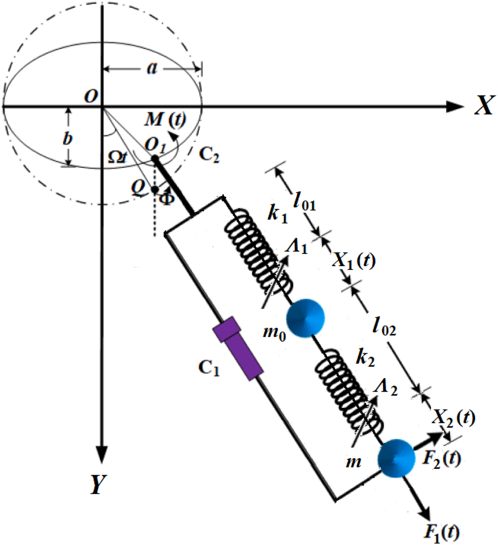
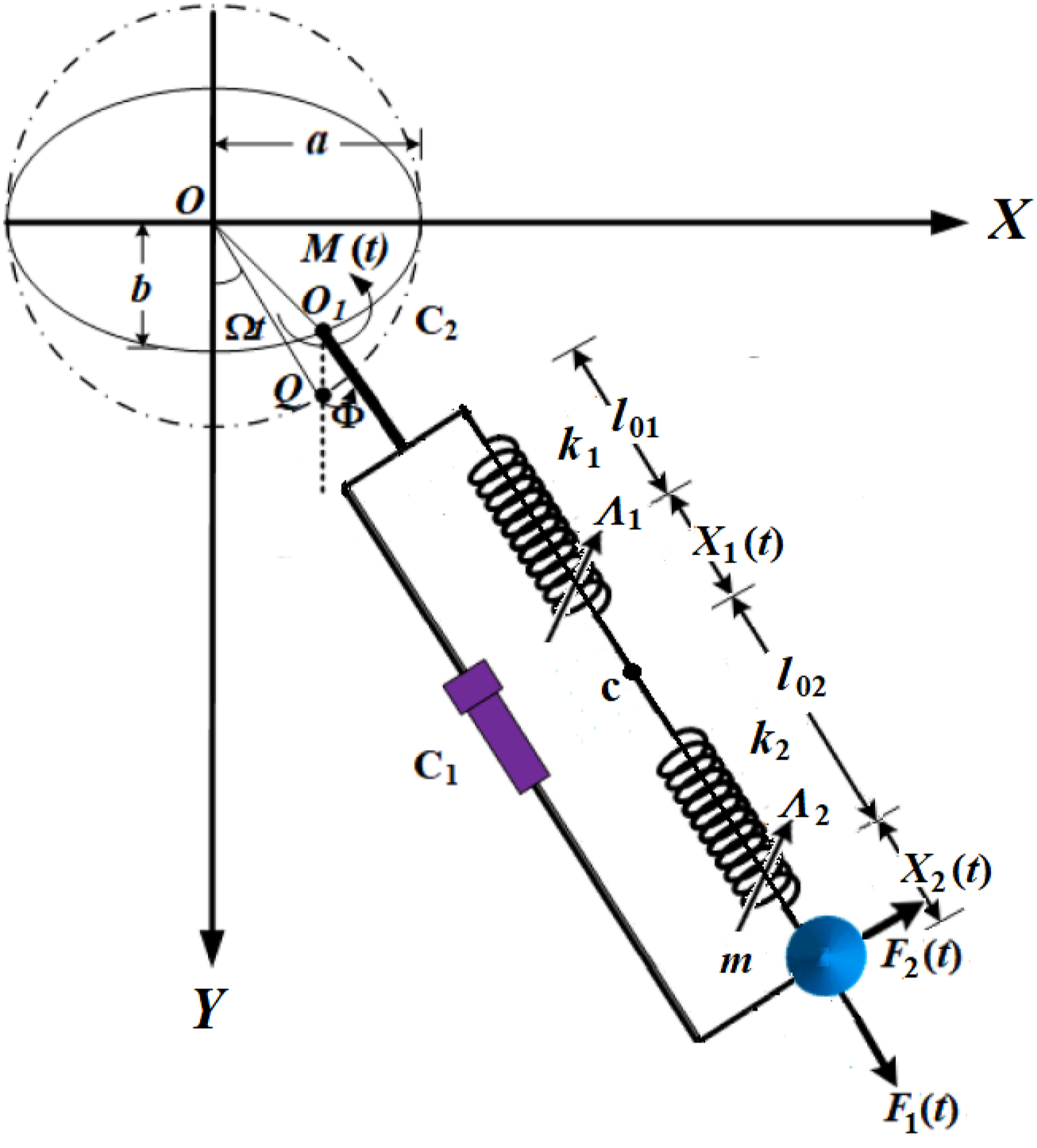
This section presents a full description of the structure of the examined dynamical system and the derivation of its EOM is the dimensionless form. This system consists of two tiny sliding particles on a bar, with masses and , in which the motion is limited to be in the vertical plane, as depicted in Figure 1. These particles are connected by a spring, and the pin point of the bar is restricted to move in an elliptic trajectory with the constancy of its angular velocity . The major and minor axes of this trajectory have semi-lengths of and to axes and . It must be noted that on the auxiliary circle , the point corresponds to .
Non-linear dynamical system.
One of these masses is connected to a point via the second spring, where the springs’ lengths at are and , respectively. The system’s motion is subjected to two applied harmonic forces on the mass , along the radial and transversal directions of the spring, and an anticlockwise harmonic moment at . Here , , and , , are the frequencies and amplitudes of and . It is presumed that the nonlinear effects on the total elasticity force are negligible, and the bar, the springs, and the dampers are considered to be massless. In this system, the coefficients of the two viscous dampers are and .
It is noted that 3DOF are available for the system, where the balls’ positions and the rotatory angle are defined by the system’s generalized coordinates. For every spring, the correlation between axial extension and the elastic force can be expressed as follows:
where and are the elastic coefficients of the springs and is its total elongation.
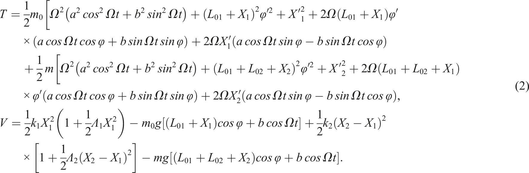
The following is the system’s kinetic and potential energies:
Here, the derivatives regarding time are represented by dashes.
Referring to this equation, we can establish the system’s Lagrangian , leading to the subsequent derivation of the mentioned equations:
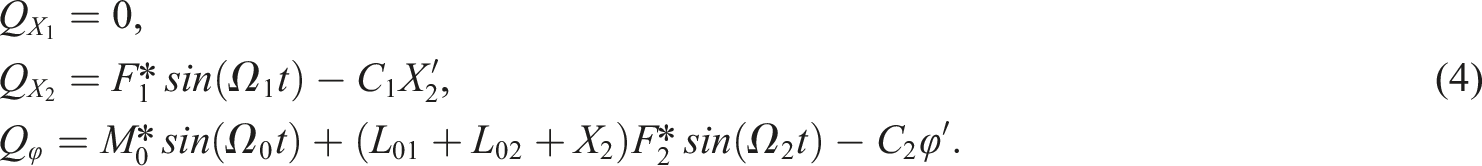
where represent the generalized forces, which consist of the harmonic forces and the damping ones. These forces have the following forms:
Furthermore, the symbols and denote, respectively, the generalized coordinates and velocities.
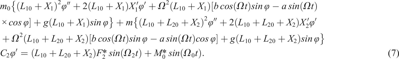
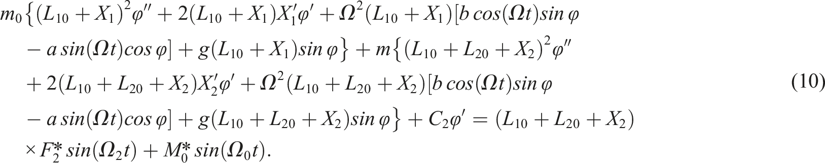
Substituting (2) and (4) into (3), we obtain the EOM:
According to equations (5)–(7), the governing EOM for the spring pendulum consists of connected two nonlinear springs in series, can be derived. Figure 2 illustrates such a system, which represents the paper’s topic. The symbol designates the spring’s connecting point, which can be thought of as the particle’s massless counterpart with a mass that tends toward zero. As a result, the point maintains its mobility along the bar. Formally, the only difference between the drawn systems in Figures 1 and 2 is the inclusion of the ball with mass . Accordingly, if we assume that in equations (5)–(7), we obtain the following:
Three DOF dynamical system of a serial pendulum’s configuration.
The equilibrium circumstance for both springs’ forces is described by the algebraic equation (8). The differential-algebraic equation (8) through (10) regulates a class of dynamical systems, which represents the corresponding model of these equations. For computational reasons, eliminating the coordinate strictly is not a good idea; therefore, both coordinates are required to clearly represent the system’s state. If equation (8) represents constraints, the coordinate can be considered complementary rather than independent. Consequently, the mechanism depicted in Figure 2 has 3DOF.
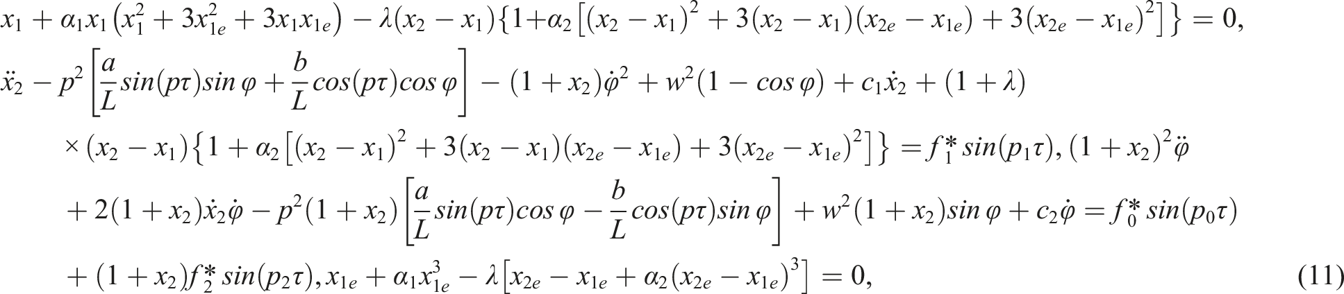
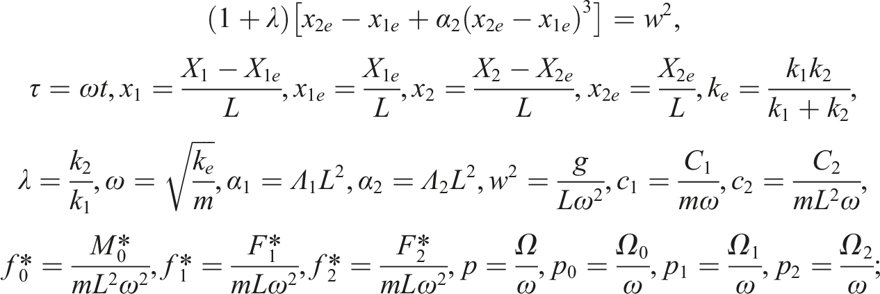
The dimensionless version of the controlling framework for EOM is structured as follows:
where and are dimensionless static extensions
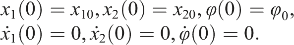
The dimensionless parameters are indicated, and the differentiation with respect to is represented by the dots. In this context, the initial conditions for both the generalized coordinates and their first derivatives are provided below
Perturbation’s methodology
In this section, the governing system of the EOM outlined in equation (11) for the examined problem is solved analytically in the form of an approximate solution using the MMTS in the time domain. To achieve this assignment, let us approximate the trigonometric functions in till the third order by selecting only the first two terms of their Taylor series around zero as below
Assuming that the system under consideration is only weakly nonlinear, we limit the analysis to tiny values of certain parameters that describe the pendulum and its loading. Assumptions on smallness are expressed as follows:
where is a small parameter. If tends to zero, then the coefficients and are considered finite.
Consequently, the vibration amplitudes and are thought to be on the order of . Thus, let’s consider the new variables and as follows:
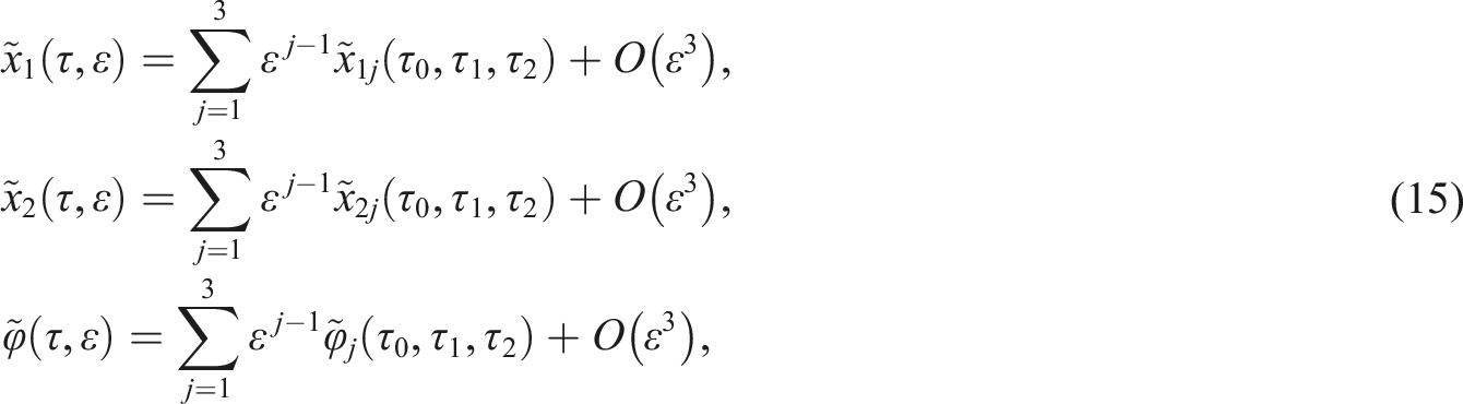
According to the procedure of MMST, we can write the asymptotic expansion of these functions as follows:
where are three variables, that are connected to the time . The upper orders have been left out because of 's modest size.
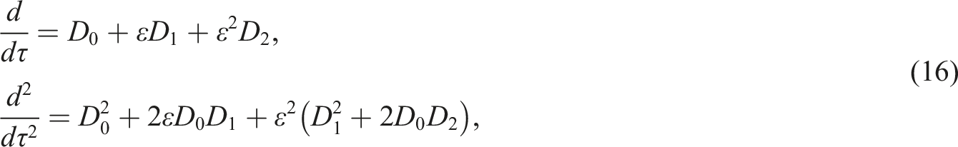
Operators having partial derivatives of the time scales are used in place of the differential operators related to time . According to the below chain rule, one writes
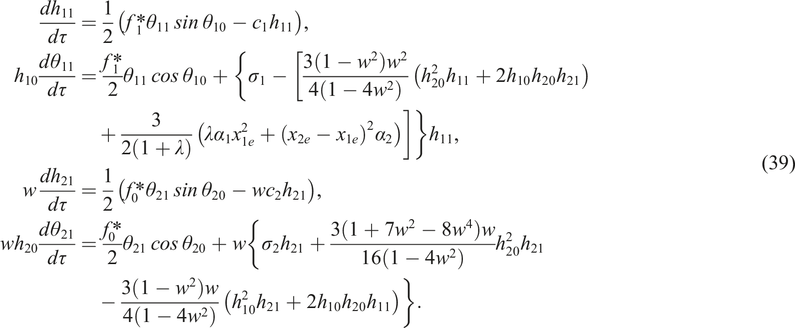
where
Owing to the presence of algebraic and differential equations, one can deal with the MMST procedure to provide the desired solutions.
Non-resonant oscillations
Substituting from (12)–(16) into (11) to generate equations involving a small parameter raised to various powers. It should be possible to satisfy all three equations for any value of . Upon organizing the equations’ terms by the magnitude of , eliminating terms of order or greater, the method of undetermined coefficients enables compliance with the condition. This process yields a collection of nine equations involving unspecified functions and , in which three distinct sets of partial DEs comprise the entire ones. The equations in the first group are those that follow, accompanied by .
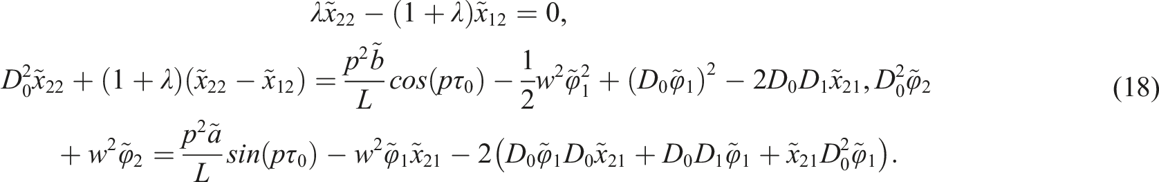
These equations are designated as the first-order approximation equations, while the terms containing lead to the derivation of equations representing the second-order approximation
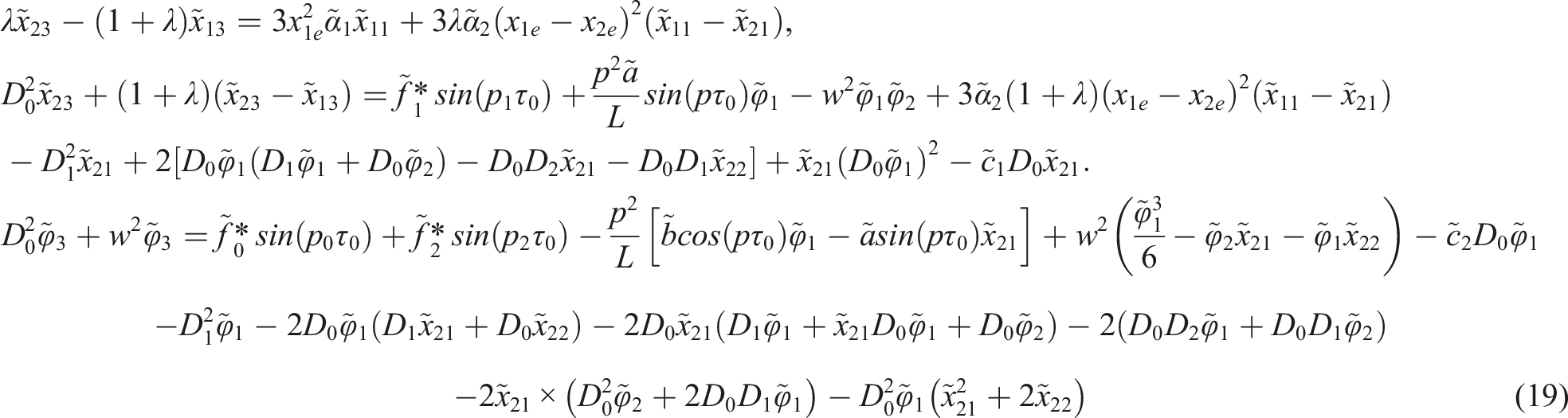
The coefficients associated with constitute the equations representing the third-order approximation
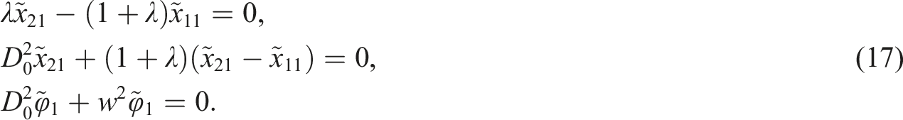
In contrast with systems regulated purely by DEs, every stage of the asymptotic approximation is expressed via a single algebraic equation. The way in which these equations are approximately solved is intricately linked to the linearity of the differential operator that arises in other equations. According to this requirement, and are linearly related. Assumption (13) justifies this rough linearization.
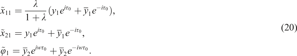
One should note that equations (17)–(19) can be solved sequentially. In the process of estimating the solution, we invariably begin with solving the algebraic equation. Thus, the general solutions for the system of equation (17) of the first group take the following form:
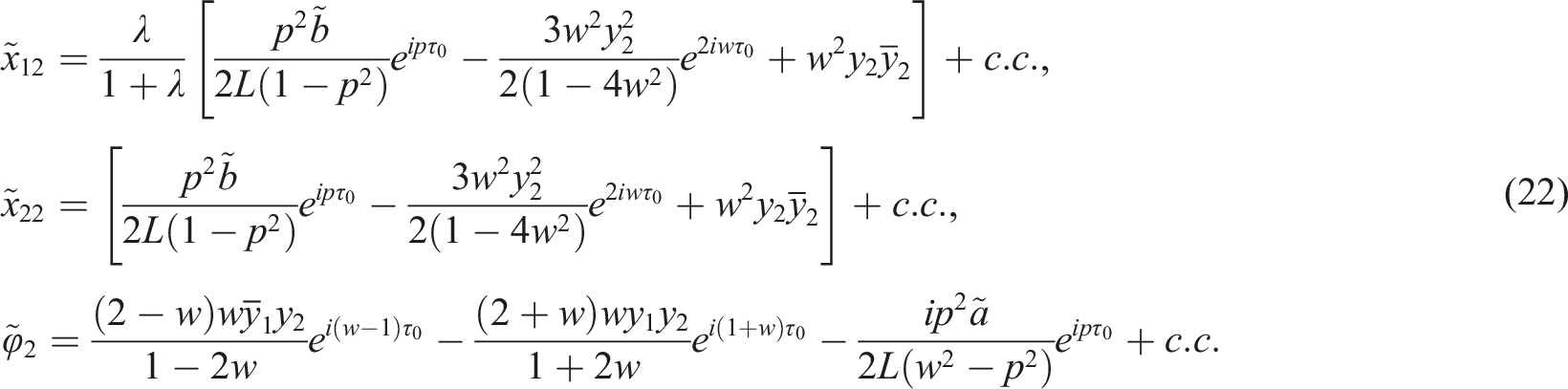
In this context, represents the imaginary unit, and together with its complex conjugate are complex-valued functions that are not yet determined, dependent on the slower time scales and . In view of the previous solutions (20) and the system of equation (18), secular terms have been obtained. The elimination of these terms required that
As a consequence, the solutions of second order are given by
In this instance, signifies the complex conjugate of the earlier terms.
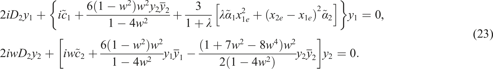
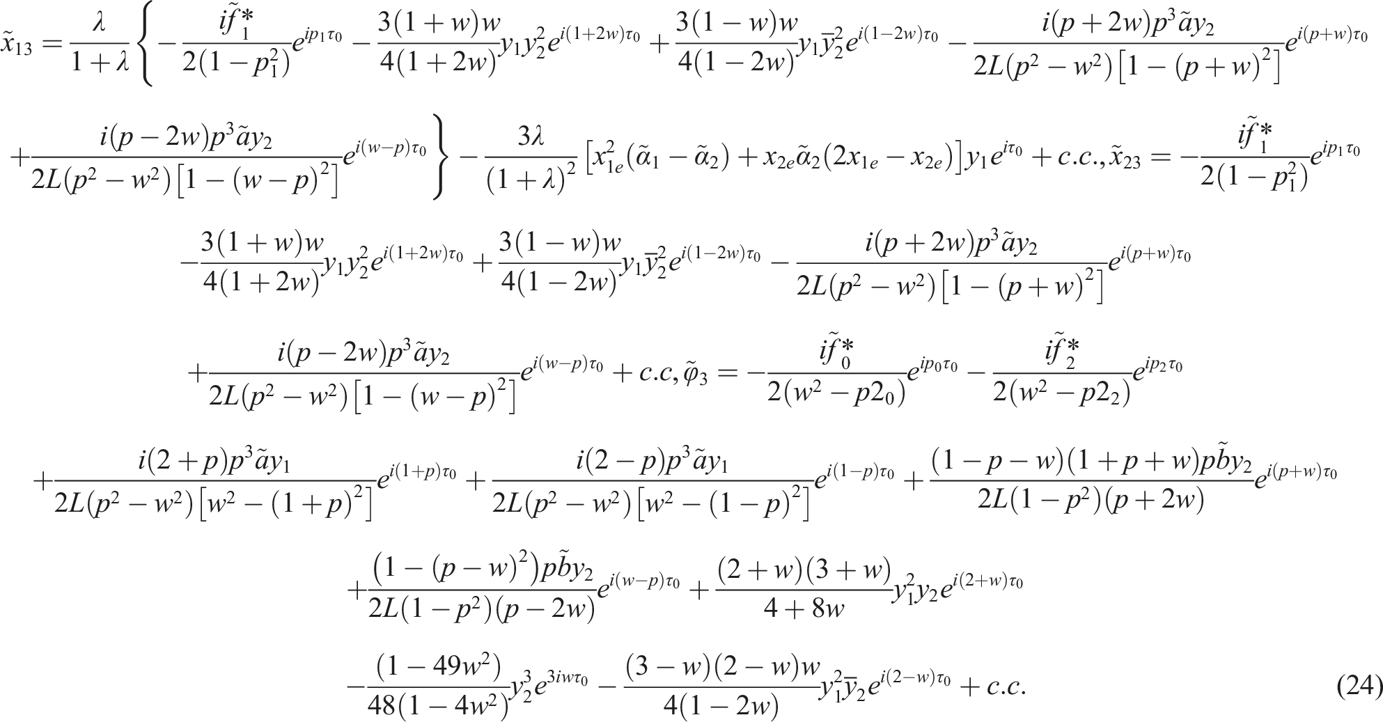
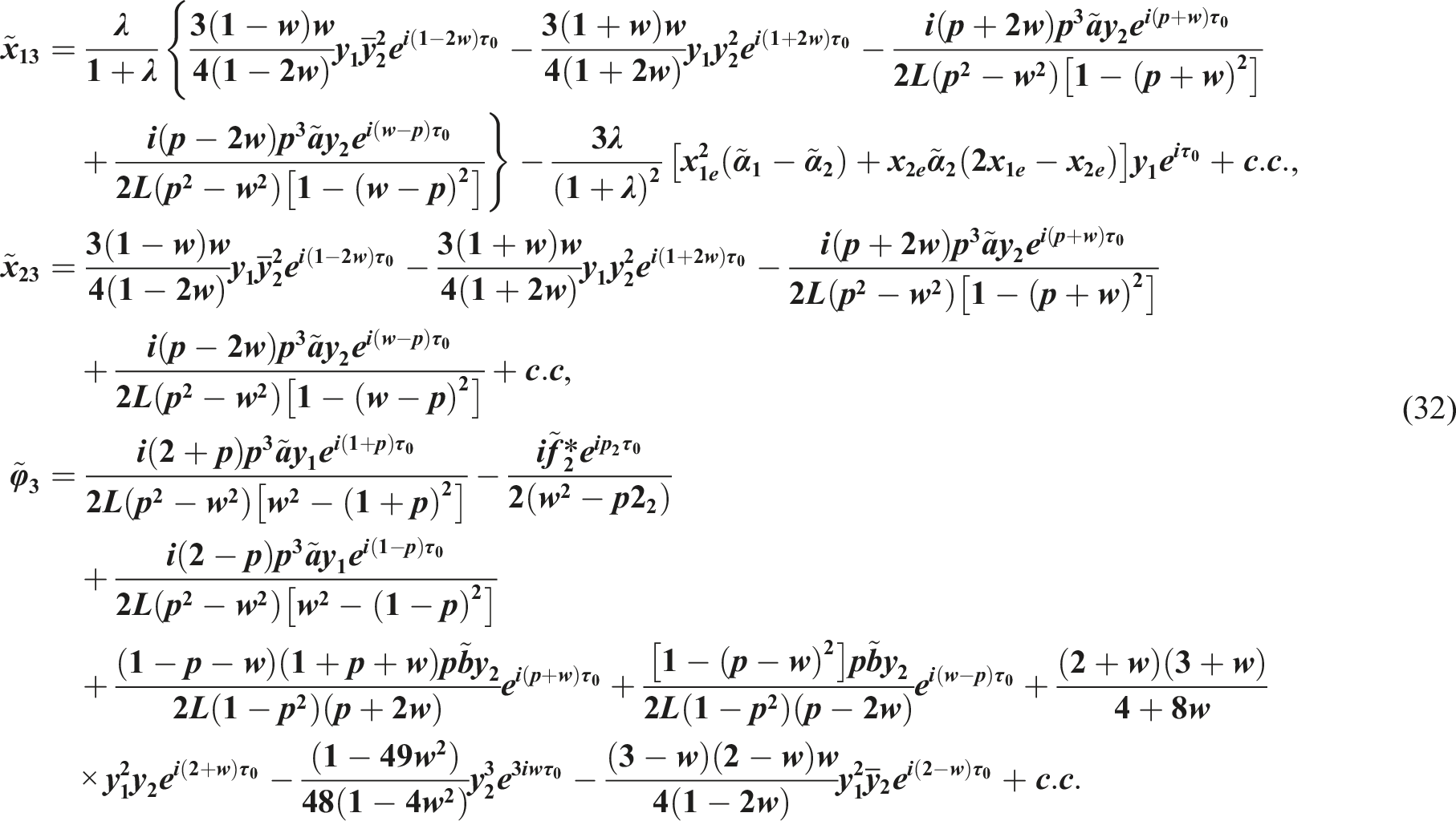
Substituting (20) and (22) into the third group (19) and removing terms that cause secular ones, the solvability conditions for the third-order approximation are obtained as follows:
Leveraging the preceding context, the solutions of third order can be written as follows:
By leveraging the assumptions outlined in hypothesis (14) and the solutions provided in series (15), along with the attained solutions in equations (20), (22), and (24), we can promptly derive the required approximate expressions of and up to the third approximation.
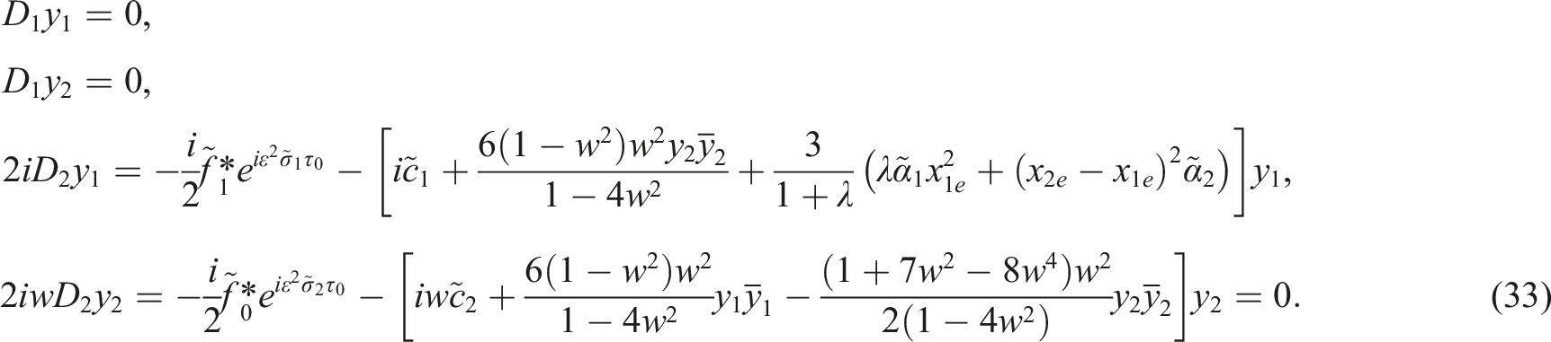
Taking into account the removal conditions (21) and (23) targeting secular terms, the functions can be estimated. From condition (21), we can deduce that the functions do not have any reliance on the variable . Bearing this circumstance in mind, we can display these functions in the next exponential form
Both functions and assigned to be real-valued.
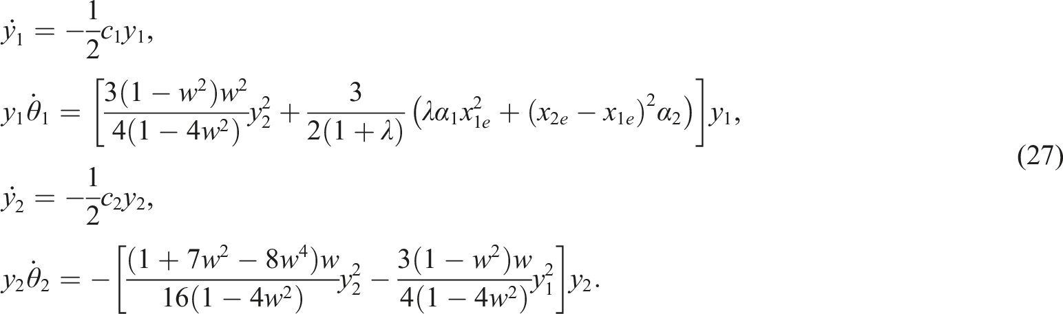
Utilizing the analysis presented above, the first-order derivatives of the functions can be summarized as follows:
Thus, the substitution into equations (25) and (26) enables the conversion of the partial DEs (21) and (23) into ordinary DEs. By distinguishing the real components from the imaginary ones, one obtains the below system of four first-order ordinary DEs concerning and .
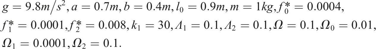
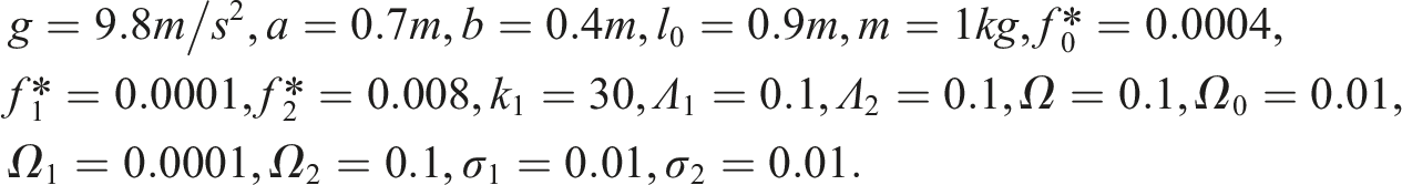
This system can be solved numerically for both and using the algorithms of Runge–Kutta in light of Mathematica software 12.3. Therefore, the next data are used
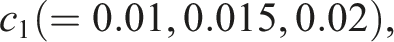
Distinct plots visually portray the solutions of the aforementioned system for the chosen values of the physical parameters, as illustrated in Figures 3–8. These figures are evaluated when the values of both damping parameters are as follows:
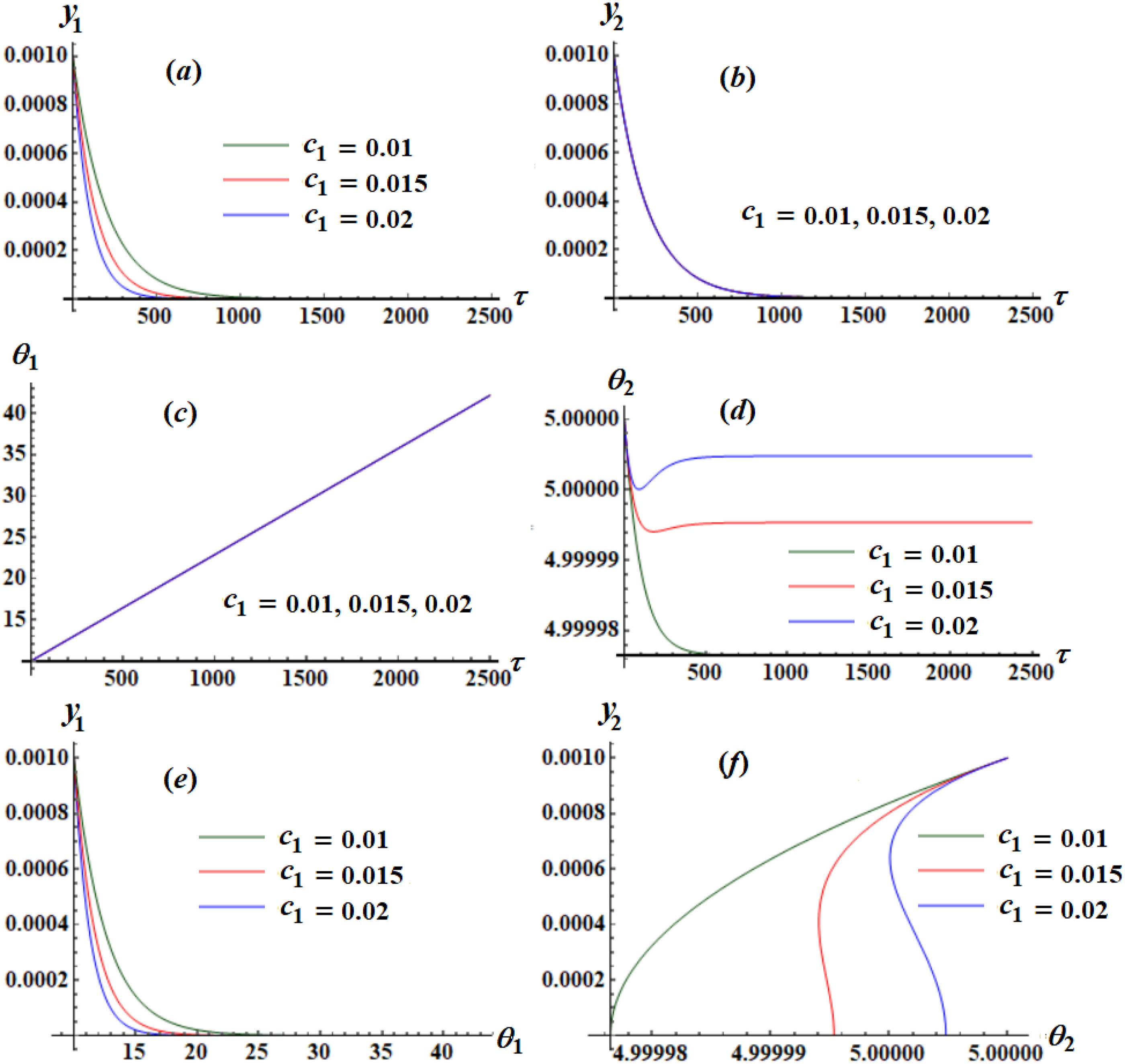
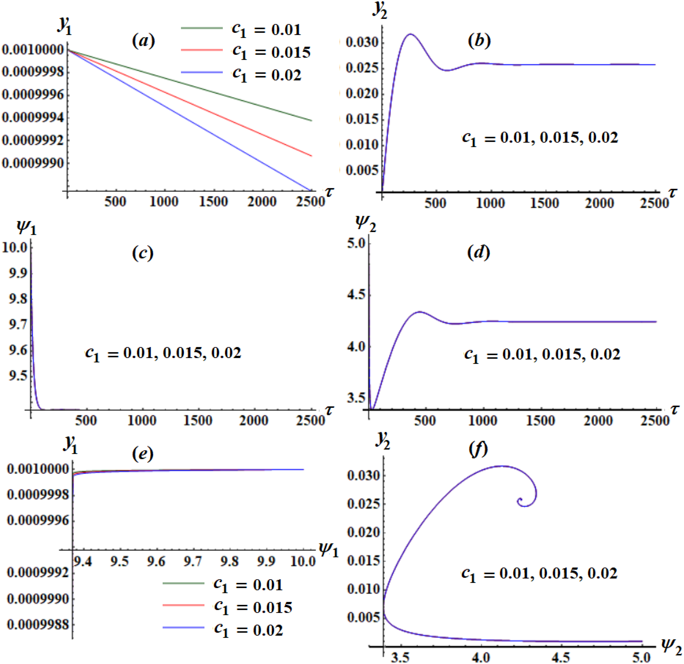
(a)–(d) shows the time variation of and the phases at , and , while (e) and (f) present their projections in the planes .
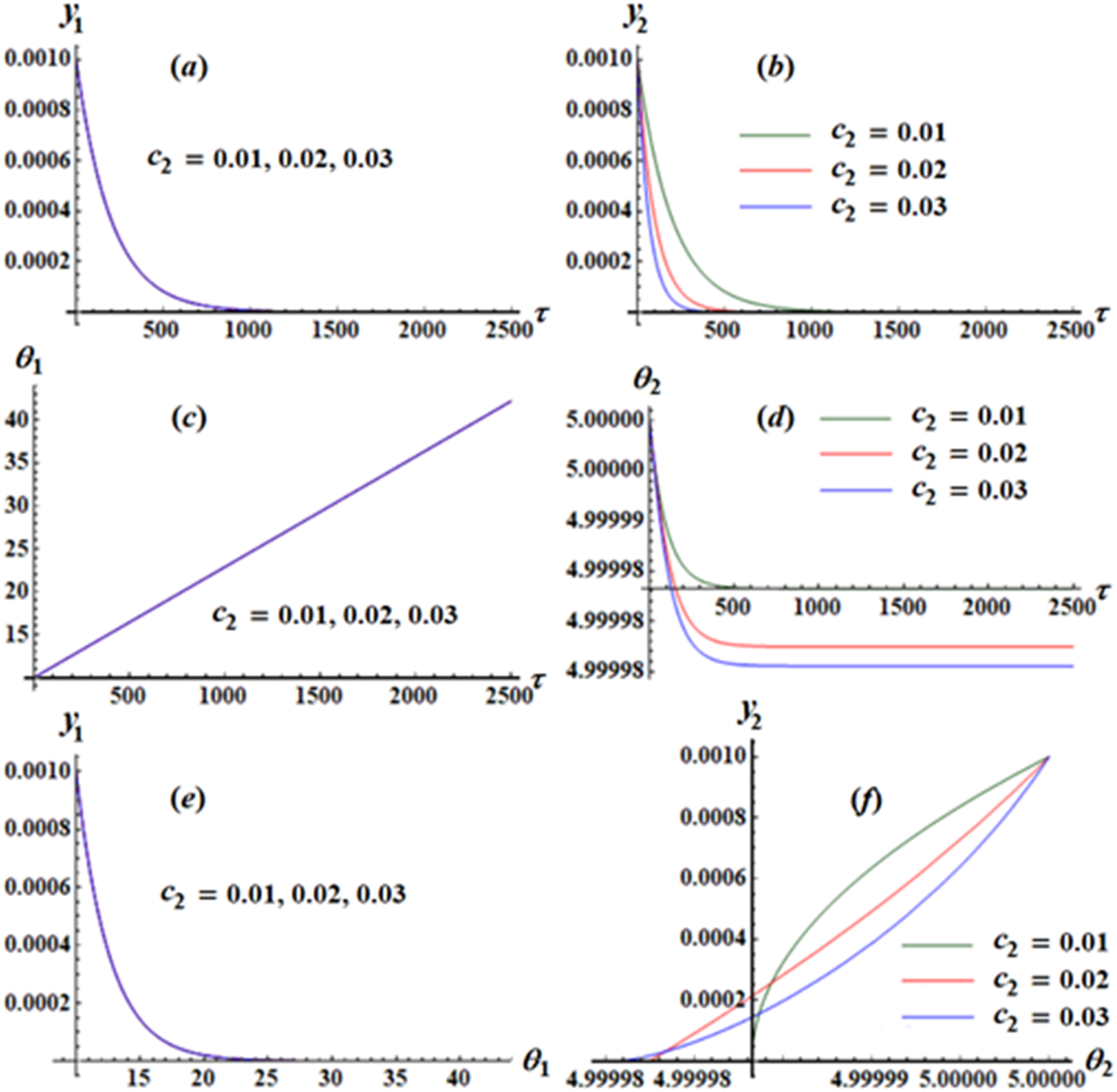
(a)–(d) shows the time variation of and the phases at , and , while (e) and (f) present their projections in the planes .
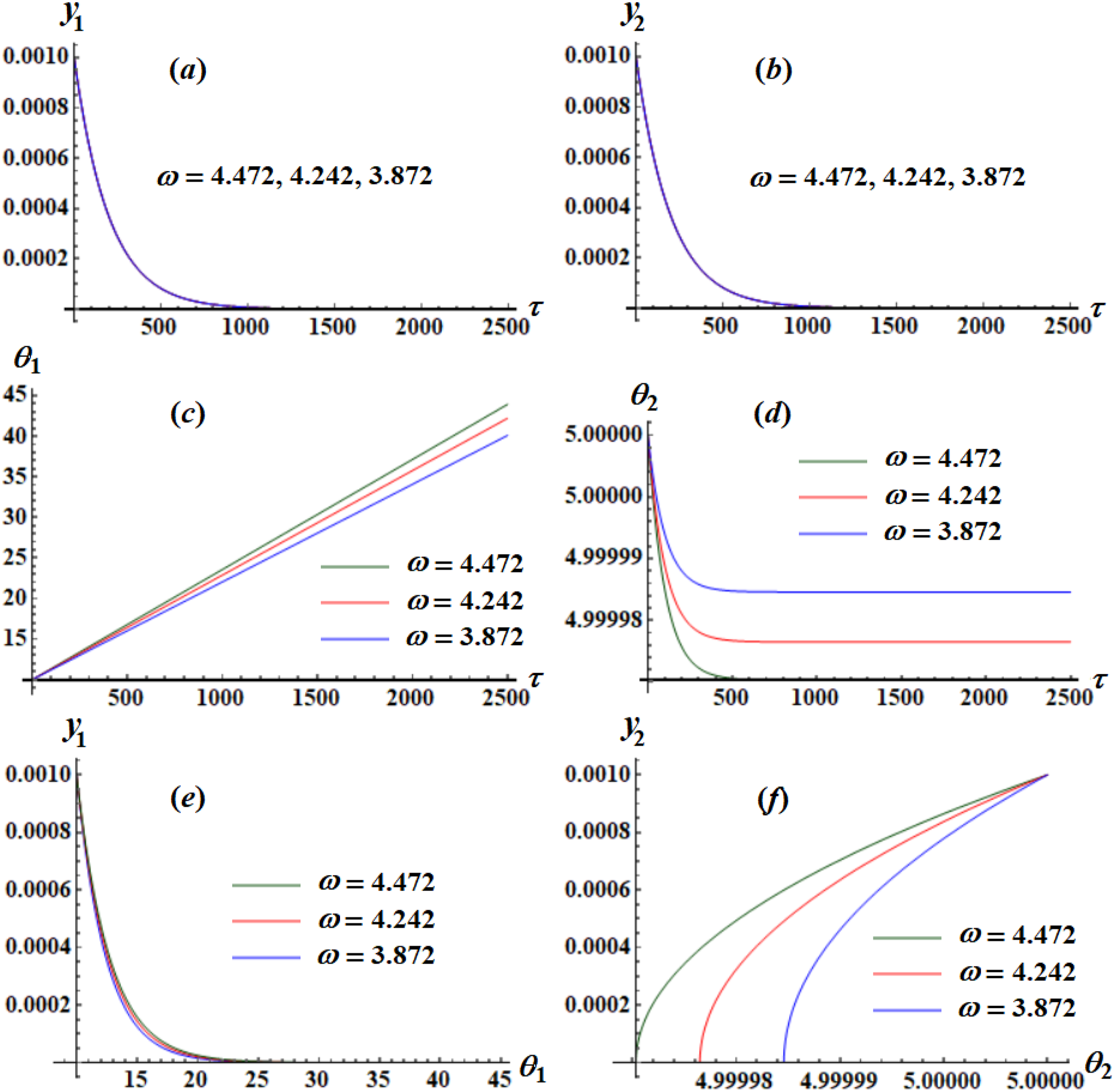
(a)–(d) presents the behavior of the functions and the phases at and , while (e) and (f) illustrate their projections in the planes .
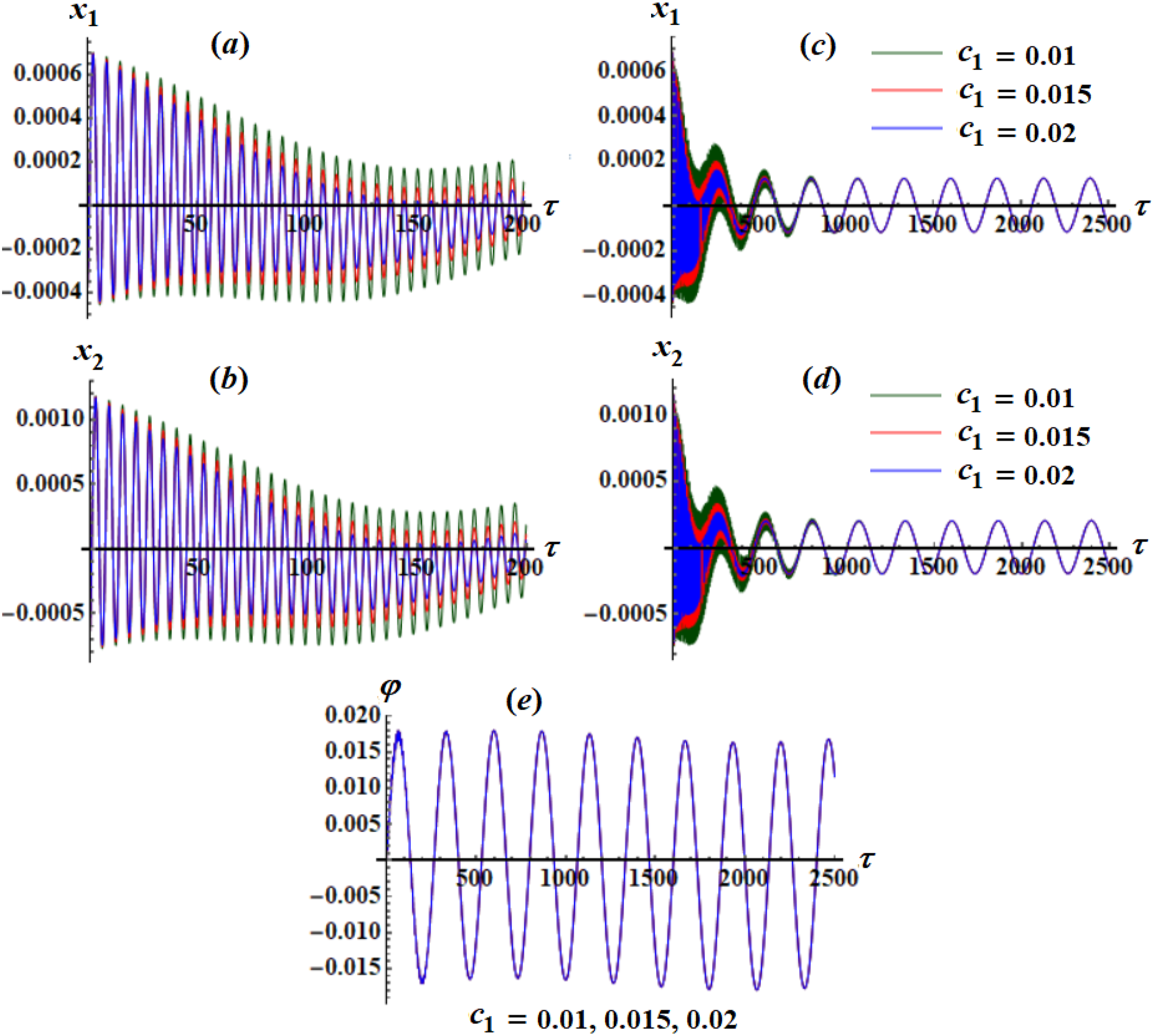
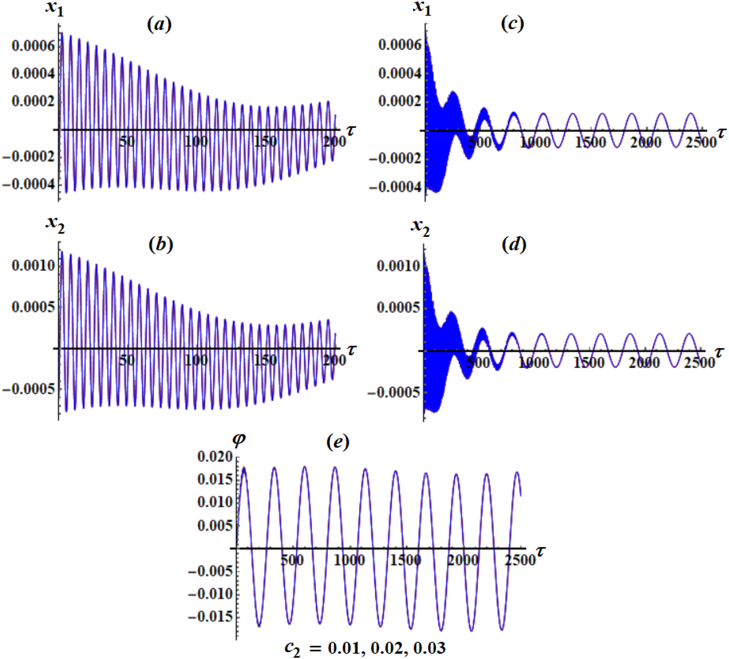
Solutions’ time histories when , and :(a) and (b) at ; (c)–(e) at .
Solutions’ time histories when , and :(a) and (b) at ; (c)–(e) at .
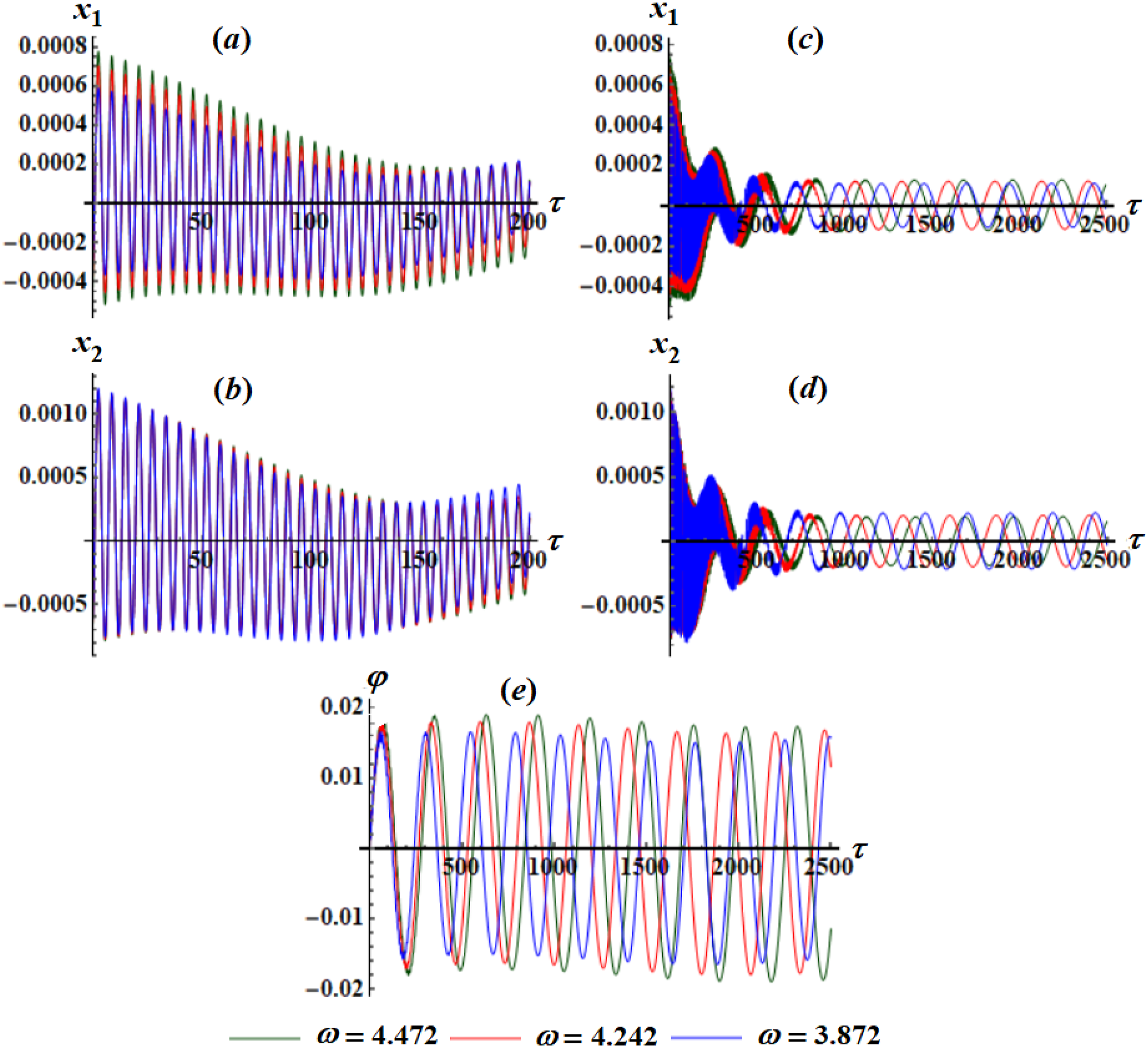
Solutions’ time histories when and : (a) and (b) at ; (c)–(e) at .
and the frequency is included. It is apparent that the plotted curves of the amplitude and the phase plane are positively impacted by the variation of values, and they have decay forms, as explored in Figure 3(a) and (d), respectively. The underlying reason is that their equations are based on the values of . On the other hand, the temporal curves in the planes and are not impacted by the change in the values of , as indicated in Figure 3(b) and (c), because the first-order equations of and don’t depend on the parameter . The projections of the included curves in parts (a), (b), (c), and (d) of Figure 3 on the phase planes and are graphed in Figure 3(e) and (f).
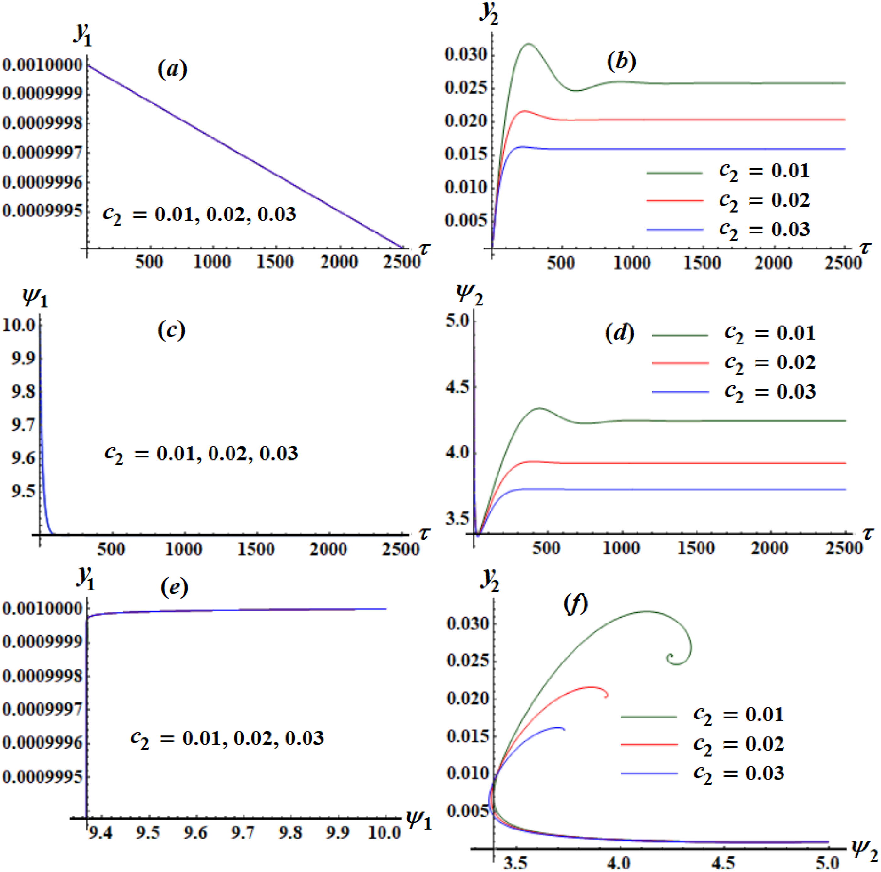
Figure 4 examines the influence of the change in amplitudes and phase angles and , respectively, when the values of have different values, as well as the study of their phase planes. It is obvious that and don’t impact with the change in values, while and vary to have decay forms over time. Furthermore, when the dimensionless time parameter is excluded, the projections of and in the plane are graphed.
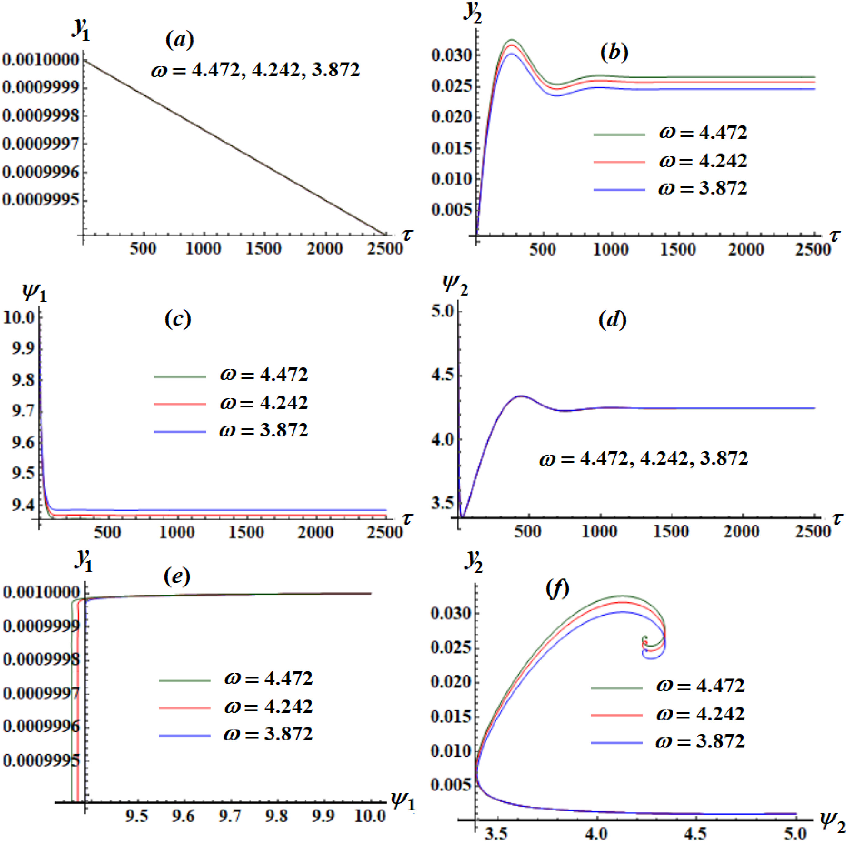
The plotted curves in Figure 5 demonstrate that they are drawn for various values of the frequency . Decay behaviors are noted in Figure 5(a), (b), and (d) when time goes on. Furthermore, the amplitudes don’t impact by the change in values, while are influenced by the same values, as seen in Figure 5(a)–(d). The curves in Figure 5(e) and (f) show the curves of the phases via amplitudes in the planes .
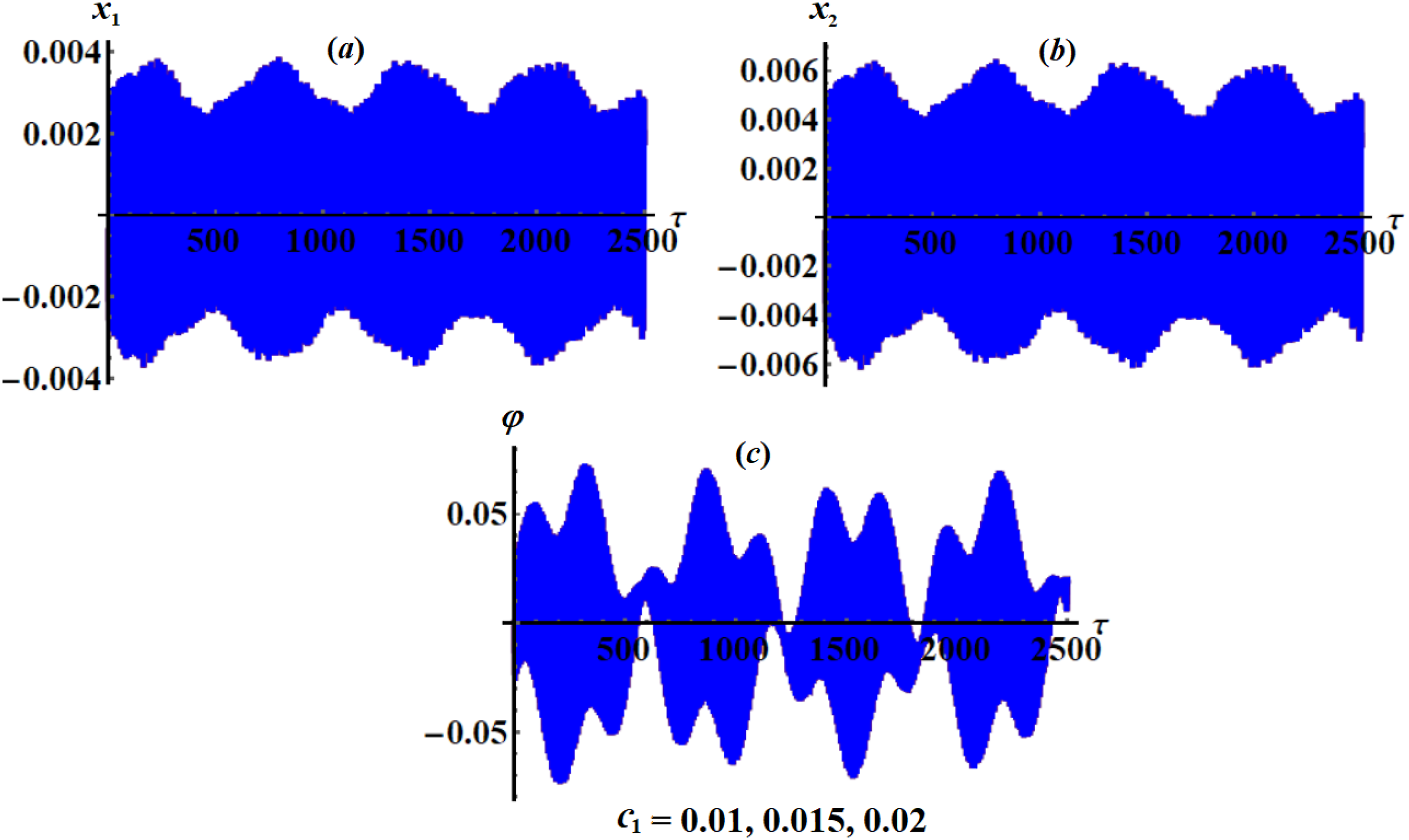
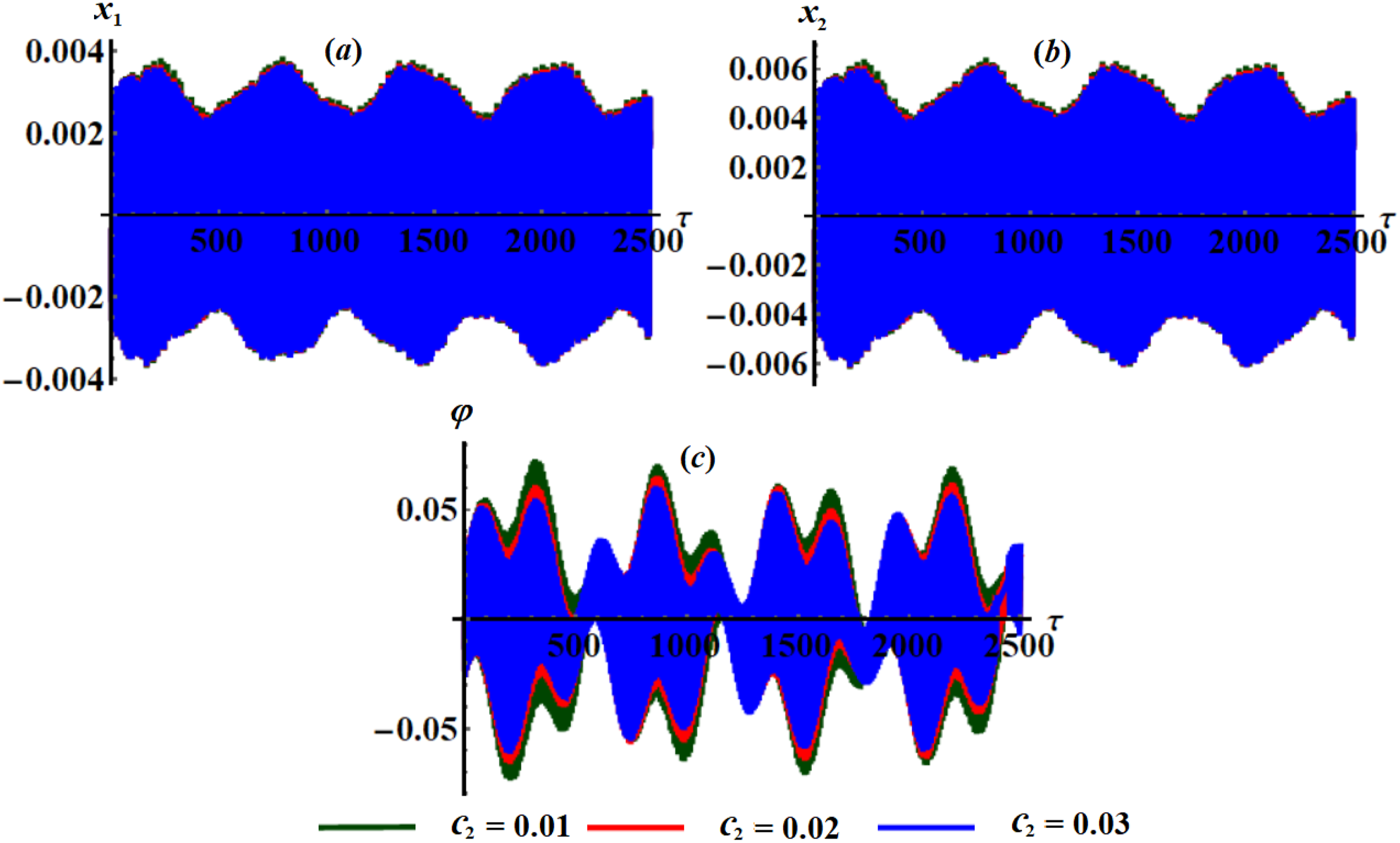
Now, we will display the identified solutions and when and have various values, as in Figures 6–8. Their portions (a) and (b) show the solutions of and in short-range, that is, , while portions (c) and (d) presented these solutions for long ranges, that is, . These solutions have decay forms through the time interval and then will be periodic till the end of the long-range interval. The analysis of the drawn curves in these figures expresses that the solutions and are influenced by the change in and , as indicated in Figures 6 and 8. On the other hand, the achieved solutions and don’t impact with the change in values, as drawn in Figure 7. This is attributed to the mathematical formulations used for the first-order equations in system (26). Whereas, the periodic solution is influenced by the change in only, as explored in Figure 8(c), where the amplitudes of the presented waves of this solution increase with the increase in values.
It must be mentioned that periodic solutions imply that the system’s behavior repeats over time, making future states predictable. This predictability is crucial for planning and control in various applications. These solutions can indicate stability in a dynamic system, meaning small disturbances or changes in initial conditions do not lead to unpredictable behavior. This stability is critical in control systems, ensuring that the system remains in a desirable state. Moreover, it can be represented as optimal operating points for dynamic systems, allowing for efficient and effective performance. For example, in power systems, periodic solutions can help optimize load balancing and energy distribution. These solutions can serve as a benchmark for understanding more complex, non-periodic behaviors, providing a stepping stone for advanced research and development.
Classification of resonance cases
In this part, we will examine how to categorize the different cases of resonance using the solutions mentioned in (22) and (24), which are applicable as long as their denominators are non-zero. Accordingly, these cases are divided into primary external resonance at ; internal resonance at ; and combined resonance at .
Our focus will be on two primary external resonances. Thus, we include the occurrence of both cases simultaneously.
Relation (28) reveals the closeness of to and to , respectively. To accomplish this, one can introduce the dimensionless values defined by the detuning parameters (indicating the gap between the oscillations and the precise resonance) as follows:
Under the assumption that the parameters are of order , we can write
where the coefficients are finite as tends to zero.
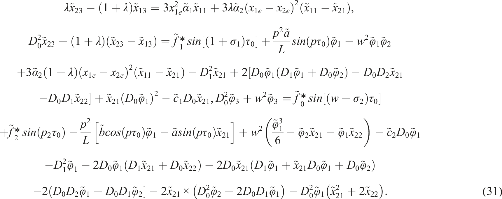
Substituting (29) and (30) into (11) and using (13)–(16), and then equalling the coefficients of the , we obtain three groups of equations according to the various powers of . Two of them are the same of the systems of equations (17) and (18), while the latter group has the below form
Based on the solutions (20) and (22), one can obtain the solutions of the third group of approximation (31) after removing the yielded secular terms in the form
The eliminating conditions of secular terms are given below
An in-depth analysis of the aforementioned solvability conditions indicates the presence of a system of four nonlinear partial DEs related to the functions that vary with the slow scales . After that, we may present these functions’ polar forms and their first derivatives as in (25) and (26), respectively.
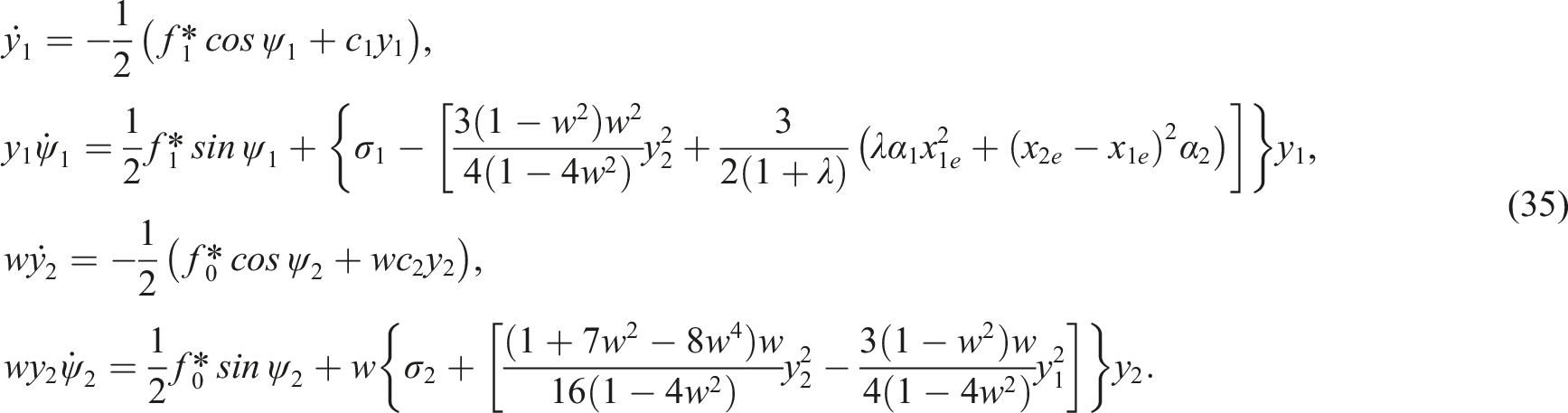
Hence, by applying equation (25) and the subsequent modified phases, we can convert partial DEs (33) into ordinary ones
when the imaginary and real parts are separated, the resulting system consists of four first-order ODEs involving and . These equations are known by the ME of the examined model when two resonance scenarios are taken into account
According to the system of equation (35), one can solve it numerically using the Mathematica 12.3 to obtain the solutions and when the following data are considered:
These solutions are graphed beside the phase plane diagrams for the projections of these solutions in the planes , as in Figures 9–11. These graphs are calculated when the and have the values and , respectively. It is noted that the temporal history of the amplitude has been impacted by the variation of values, while and don’t have any change with the same variation, as seen in Figure 9(a)-(d). It is observed that the wave sequence ranges between decreasing waves, which are represented by straight lines, as in Figure 9(a), and between ascending waves for a certain period of time, then they begin to decrease, and then they are stable until the end of the time period, as in Figure 9(b) and (d). Moreover, we also observe that one of the waves tends to decrease sharply until it reaches near the horizontal axis, which represents time, and the wave then stabilizes, as in Figure 9(c). When the time is excluded from the amplitudes and the related phases , one obtains a projection of them in the planes , as seen in Figure 9(e) and (f).
(a)–(d) shows time change of the functions and while (e) and (f) show the curves in the planes at when , and .
(a)–(d) reveals the behavior of and , while (e) and (f) reveal the curves in the planes when at and .
(a)–(d) portrays the change of the time-dependent functions and , while (e) and (f) portray the curves in the planes when at .
With an insight into the curves drawn in Figure 10, we find that these curves, which represent the amplitude and the phase , were affected by the change in the values of , as in Figure 10(b) and (d), respectively. Therefore, their phase plane curves undergo a similar change as in Figure 10(f). On the other hand, we find that the curves representing and did not have any significant effect on changing the values of , as in Figure 10(a) and (c). Consequently, the corresponding phase plane plots for them do not change with the variation of . The behavior of the drawn curves in portions of Figure 10 is considered very close to the behavior of the plotted ones in Figure 9. This can be traced back to the mathematical representation found in the system of equation (35).
By examining the curves in various parts of Figure 11, we observe that the previously mentioned frequency values significantly impact both and , as shown in Figure 11(b) and (c). Conversely, the effect on is minimal or almost imperceptible, as indicated in Figure 11(a). Additionally, there is no observable effect of changing frequency values on the behavior of the wave representing , as noticed in Figure 11(d). Consequently, the projections of these curves in the planes are influenced by the changing frequency values, as illustrated in Figure 11(e) and (f). The behavior of the drawn waves is consistent with the behavior observed in the previous Figures 9 and 10.
Taking a closer look at the curves in Figure 12, one can observe that the solutions and exhibit a wavelike nature, with all their behaviors consisting of wave packets. The shape of these packets varies depending on the specific solution they represent. These waves are calculated when and at aforementioned various values of . Furthermore, changing the values of the damping coefficient does not affect the drawn waves, which is expected since these solutions do not explicitly depend on .
Solutions’ time histories , and in parts (a), (b), and (c), respectively, when , and .
In the same context, parts of Figure 13 are plotted at and while varying as previously mentioned in Figure 10. A noticeable change is observed in the waves representing the solution as a result of changing the values of , as indicated in Fig. (13(c). Moreover, the amplitudes of the waves decrease as values increase, while the wavelength remains constant. There is a slight change in the behavior of the waves representing the solutions and when the damping parameter varies, as presented in Figure 13(a) and (b), respectively.
Time behavior of the solutions and in parts (a), (b), and (c), respectively, when and .
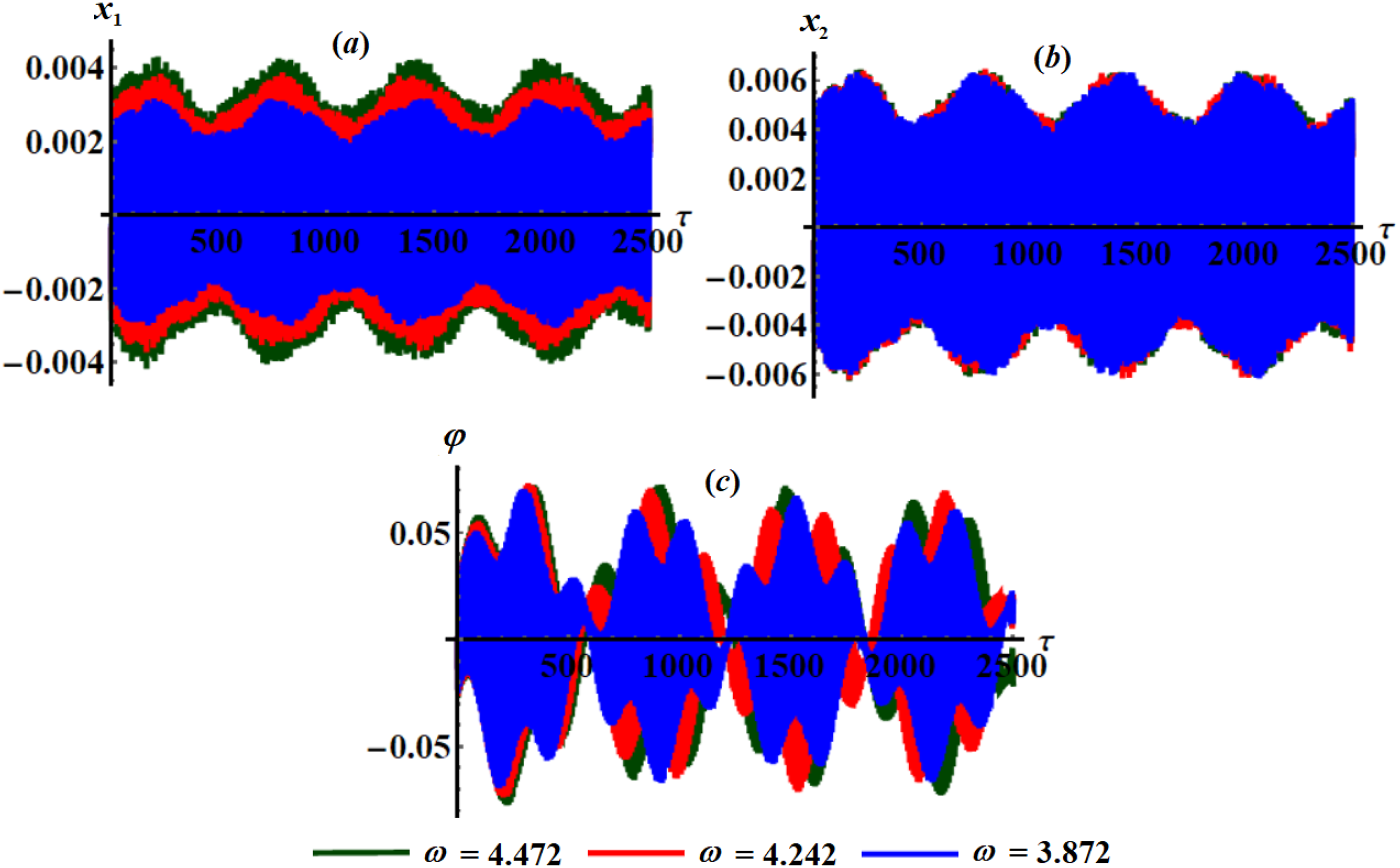
The advantageous effect of varying frequency values on the behavior of the solutions and is illustrated in the curves drawn in Figure 14. These curves are graphed considering the values and . It is evident that the wave amplitudes rise as the values of increase, while the number of waves and the corresponding lengths remain unchanged.
Behavior of the time dependent functions and in parts (a), (b), and (c), respectively, at and .
Steady-state solutions
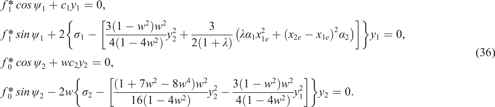
The key objective of this section is to analyze the oscillations of the examined system at the steady-state scenario when two resonance cases are examined simultaneously, that is, . Accordingly, we assume the left-hand sides of the equations in the system (35) to be zero30 in order to find the fixed points for the amplitudes and the phases . Consequently, setting , we establish the subsequent algebraic system, which includes four equations involving the functions and .
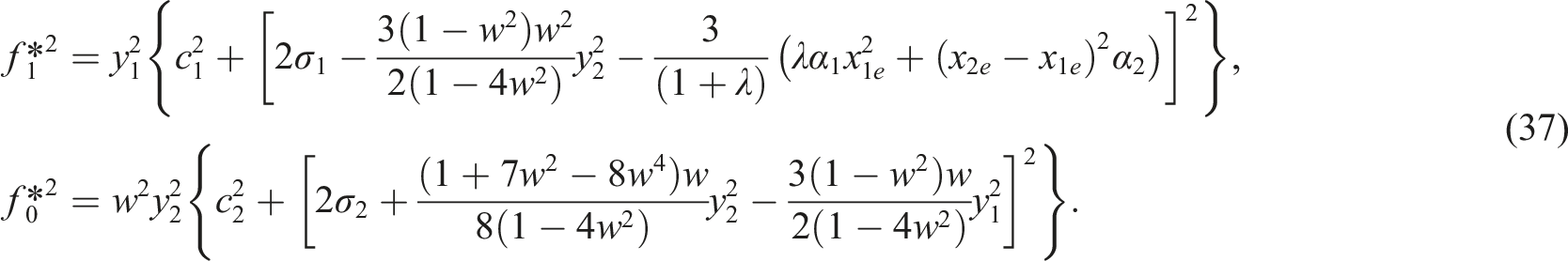
Thus, we exclude the modified phases from the previous system, resulting in the below two non-linear algebraic equations regarding and
The actual solutions of system (37), with specified values of and , as well as , represent the steady oscillation amplitudes. By varying the values of , one can identify the resonance response curves. However, the assessment of stability plays a crucial role in studying vibrations at steady-state. To investigate this further, the system’s behavior near its fixed points is examined. Consequently, the substitutions detailed below are applied in equation (35) for this specific purpose
Here, and represent the steady-state solutions, while and correspond to relatively small disturbances relative to and . Consequently, due to linearization and the fixed points of (35), one obtains
Given that and are perturbed functions of the amplitudes and phases in the linear system mentioned above, one expresses their solutions using the linear function in exponential form, where and are constants and the perturbation’s eigenvalues. To ensure the asymptotic stability of the steady-state solutions, the roots’ real components of the characteristic equation in (39) are negative31
where are given in terms of and , as follows:
For certain steady-state solutions, the conditions required and sufficient for achieving stability at the steady-state solution can be outlined according to RHC32 as follows:
The most direct feedback from applying the RHC is determining whether a system is stable or unstable. The stability of the system is assured if all elements in the first column of the Routh array have the same sign and none are zero, while the system is unstable if any element in the first column of the Routh array changes sign. By applying these criteria to systems with varying parameters, one can analyze how changes in system parameters affect stability. This sensitivity analysis helps in designing systems that remain stable under different operating conditions. The benefit from the stability RHC is valuable in control system design. It helps in tuning the controller parameters to achieve the desired stability margins and ensure robust performance. By systematically applying the RHC, researchers can make informed decisions about the design, analysis, and tuning of dynamic systems to ensure desired stability and performance characteristics.33,34
The stability analysis
In this section, we apply nonlinear stability analysis for the RHC to investigate the dynamic behavior of the studied oscillating system.35 The system’s motion is examined by considering the force acting on the spring’s direction and the moment at the pivot point . Stability criteria are implemented along with simulations of the system’s equations. It is found that the parameters of detuning , frequency , and coefficients of damping are crucial factors influencing stability. To determine the stability ranges of system (37), various system settings were tested through a predetermined process.
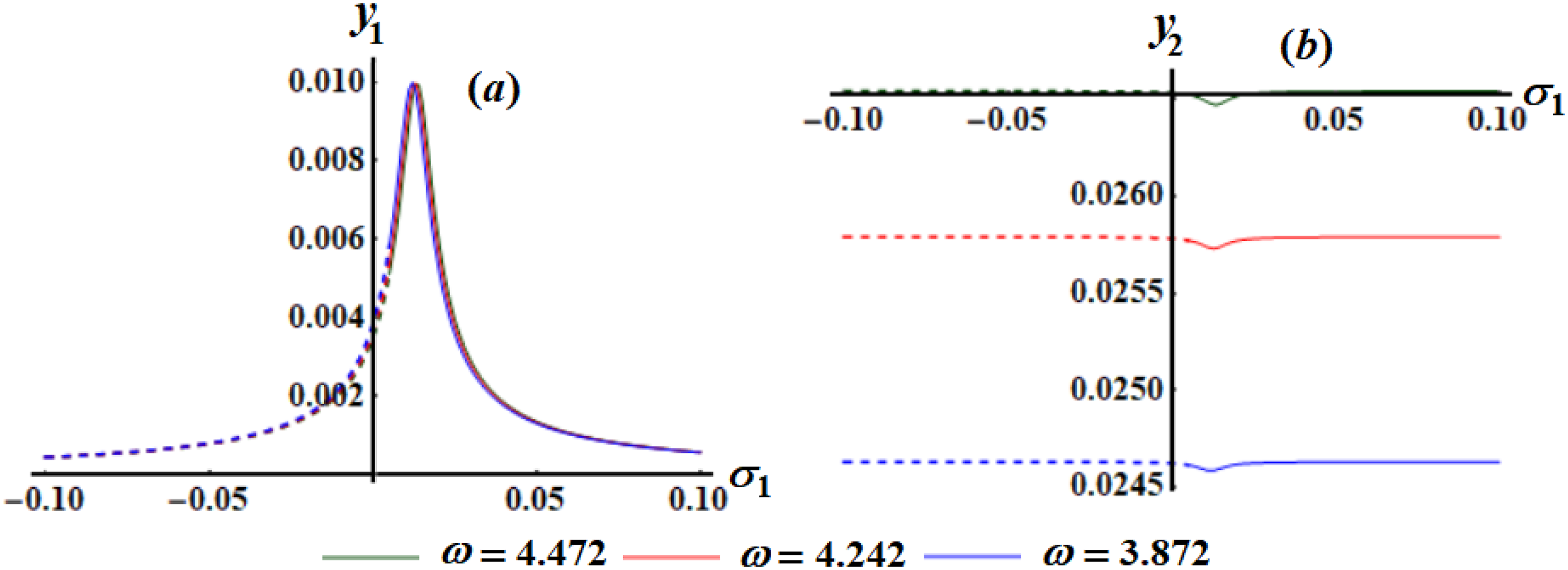
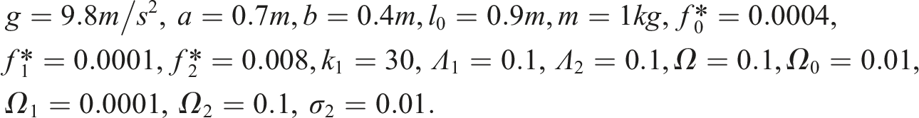
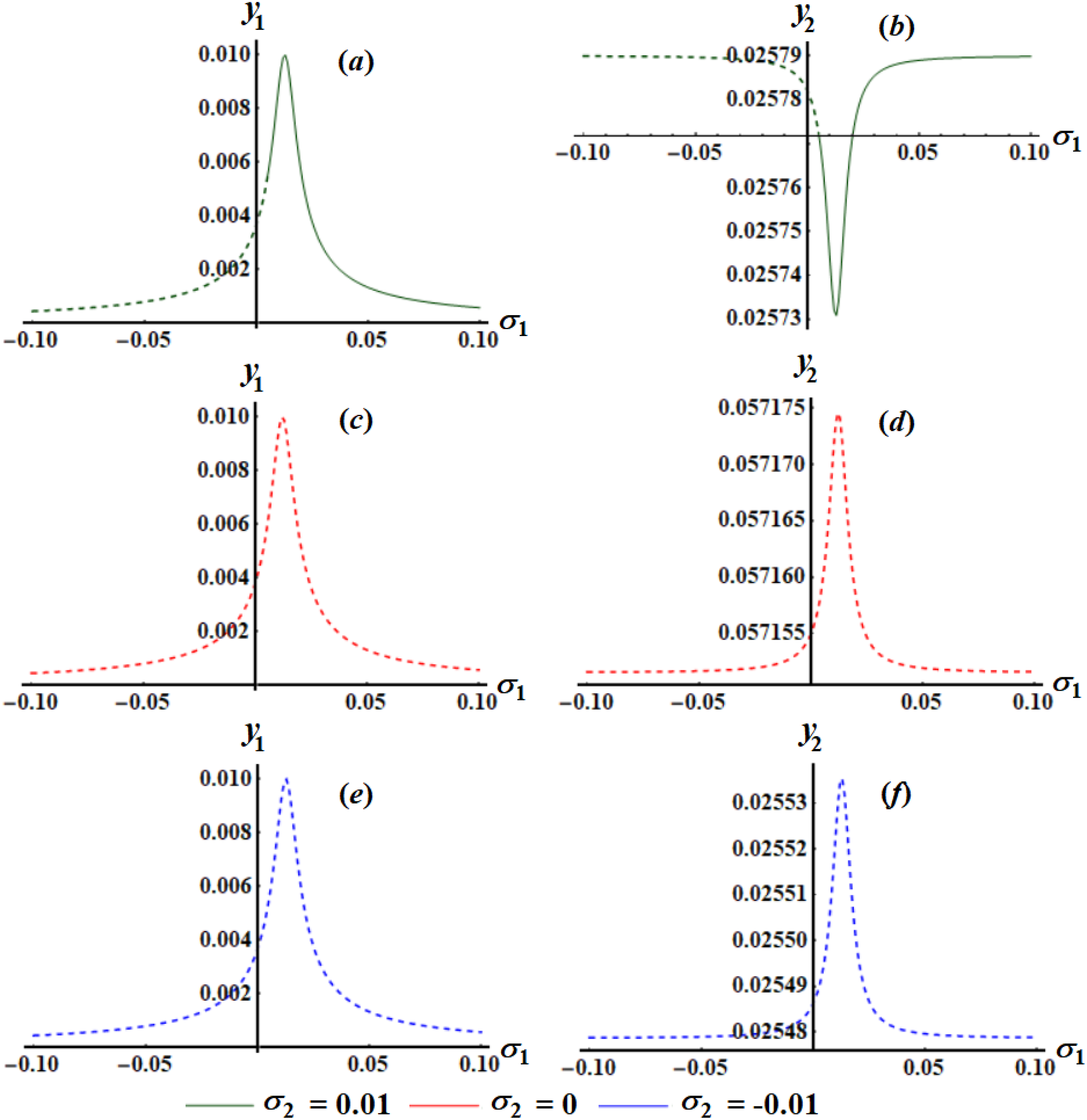
Figures 15–17 show the FRC of against concerning the system’s fixed points. They are plots depicting the time-dependent changes in amplitudes across various parametric regions when the following data are considered:
FRC of the planes at when and : (a) in the plane , (b) in the plane .
FRC of the planes at when and : (a) in the plane , (b) in the plane .
FRC of the planes at when and : (a) in the plane , (b) in the plane .
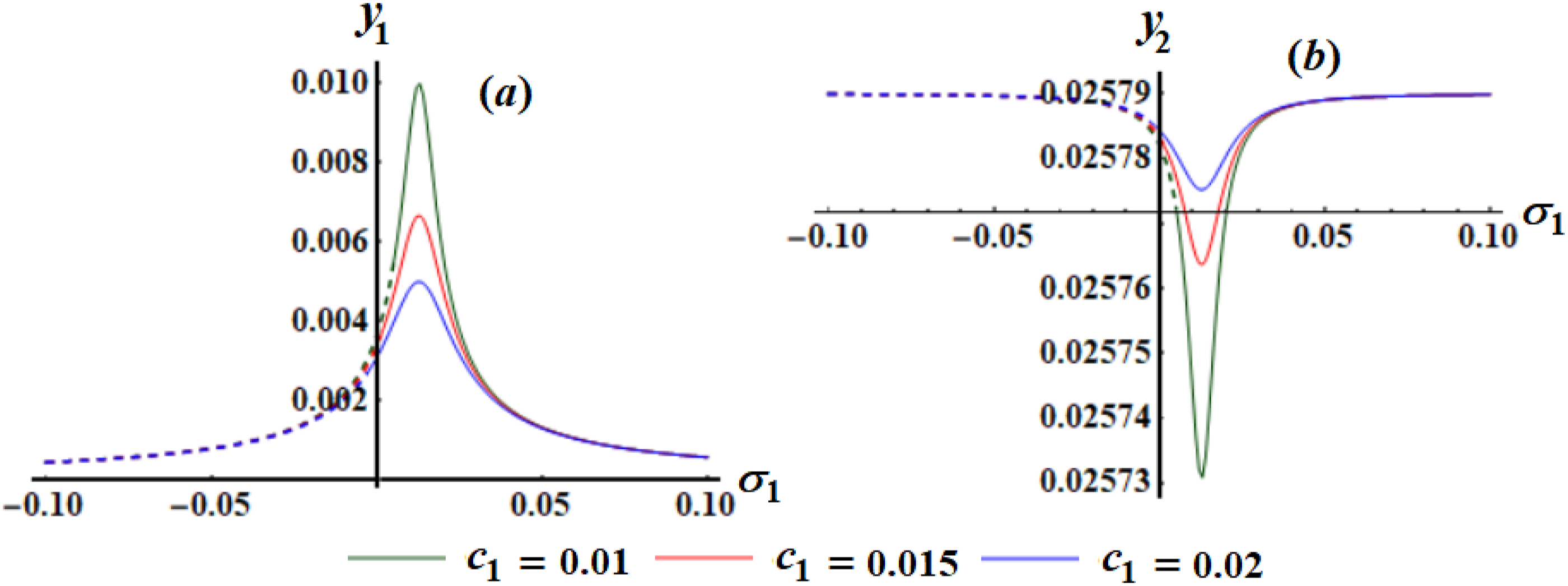
The presented stability and instability areas in Figures 15–17 are plotted when the and have the aforementioned various values. The range of is chosen to be during the interval . Based on the change in , that is, the plotted curves in Figure 15, one observes the stability zones at equals and are being in the ranges and , respectively. Whereas the instability regions at the same considered values of satisfy the inequalities and . It is noted that each curve in the parts of this figure has one critical fixed point and one peak point.
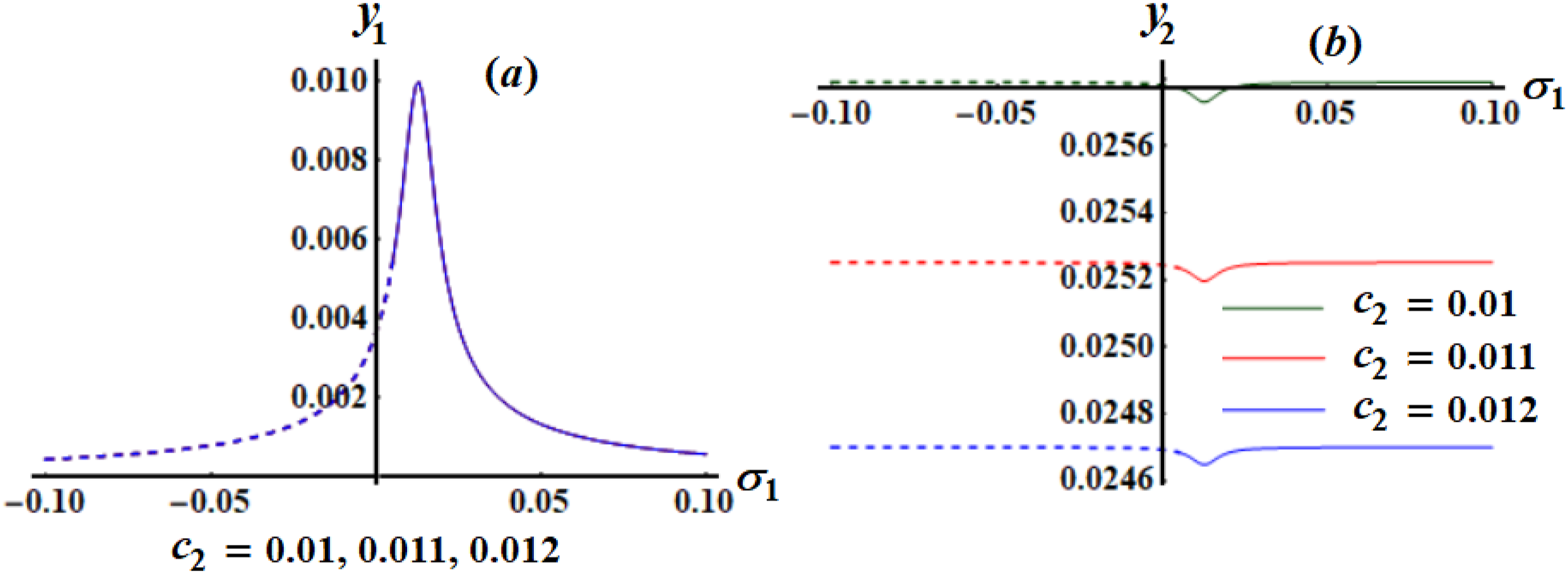
The inspection of the graphed FRC in portions of Figure 16 shows that they are calculated at , and when . It is seen that one drawn curve is calculated with the variation of values, as explored in Figure 16(a), which means that the values of this parameter don’t affect on the variation of the FRC in the plane , while the same values of have an excellent influence on the FRC in the plane , as shown in Figure 16(b). The explanation lies in the first and second equations in the system (37), where the first one is dependent on , while the second depends on . Stability zones and instability ones are matched with the inequalities and , respectively. As previously mentioned, two fixed points are observed: one peak and one critical.
The plotted FRC in Figure 17 is determined when at and at Analyzing the curves in this figure shows that these curves are impacted by the change values, in which the stable area and unstable one are found in the ranges and , respectively.
The drawn response curves in Figure 18 are calculated when at and when has the values . An examination of these curves explores that these curves are not impacted by the change values, in which the stable areas are found when at the ranges , while the unstable regions are found in the ranges . On the other hand, all the represented areas when and are unstable during the plotted domain of . The reason goes back to the fact that at least one condition of the RHC is not satisfied.
FRC of the planes when , and : (a) and (b) at ; (c) and (d) at ; and (e) and (f) at .
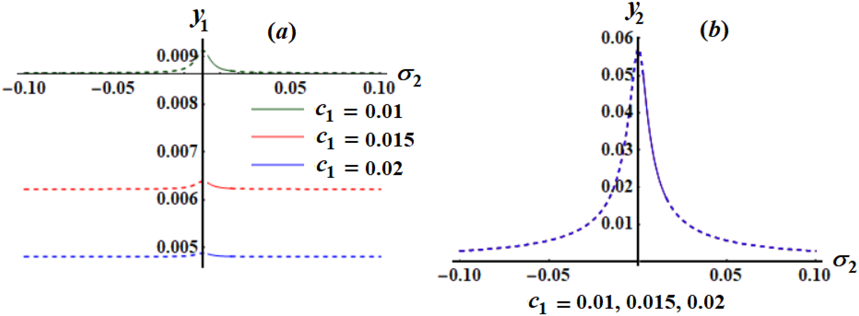
The graphed curves in Figure 19 show the FRC in the plane when have various values. These curves are calculated at and . It is noted that the domains of stable regions are smaller than those of unstable regions. The stable’s regions are found at , while the unstable ones are presented at and
FRC of the planes at when and : (a) in the plane , (b) in the plane .
Conclusion
Exploring the planar forced oscillations, a particle attached to its support point through a series of two nonlinear springs and two viscous dampers has been examined. This point follows an elliptic route due to the presence of an external harmonic force along the spring’s elongation and a viscous harmonic moment applied at the support point. The governing two differential equations have been formulated using Lagrange’s equations besides an algebraic equation. These equations have been solved for the non-resonant and resonant scenarios up to the third order of approximation utilizing the MMTS, in light of three distinct time scales. For the resonant scenarios, two cases of external resonance have been examined simultaneously. Consequently, the solvability criteria and the ME have been obtained. The RHCs have been employed to analyze the stability and instability areas for the drawn FRC. Detailed discussions and visual depictions of the motion temporal histories and stability regions are provided. These visuals highlight the advantageous effects of varying physical parameters on the system’s operational performance. The achieved outcomes are considered generalizations of those which were gained in Ref. 23 when the springs’ suspension point was stationary. These outcomes can be used to improve the design and performance of mechanical systems such as shock absorbers, suspension systems, and vibration isolators that rely on spring dynamics. Moreover, they enhance the control and stability of robotic arms and joints that use spring mechanisms to mimic muscle movements. They also optimize the behavior of landing gear systems in aircraft, ensuring better shock absorption and stability during landing.
Future work
Future work could branch out in the following several important directions to enhance both the theoretical understanding and practical applications of the studied system.
• The current study focuses can be extended to be in three dimensions, which provide a more comprehensive understanding of the system’s dynamics. Studying the role of spatial motion in the performance of nonlinear springs and dampers might reveal further resonance phenomena and intricate dynamic patterns.
• Further work could investigate the system’s behavior through higher-order asymptotic approximations, providing deeper insights into subtle nonlinear effects, especially in highly nonlinear regimes or under stronger excitations where more intricate interactions may occur.
• An obvious extension would be to explore internal resonances, where interactions between multiple natural frequencies occur, and potentially reveal novel dynamic behaviors such as mode-to-mode energy transfer or intricate bifurcation patterns.
• Exploring the effects of various damping models, such as nonlinear damping or fractional damping,36,37 could be a focus of future research. The He’s frequency and the semi-inverse method38–41 can be used to establish future results. This would improve the fidelity of real-world damping approximations and enable more accurate predictions for practical scenarios.
• Examining the system’s behavior in response to parametric excitations, where parameters such as stiffness or damping coefficients are periodically adjusted, would enable a more thorough investigation of the system’s stability limits and dynamic behavior in practical contexts like engineering applications that deal with time-varying external conditions.
• To confirm the theoretical results, experimental studies could be conducted, or the findings could be applied to real-world applications, such as vibration absorbers, mechanical linkages, or suspension systems.
• Future work could include large-scale numerical simulations that explore a wider range of parameter values, beyond the scope of the analytical approximations used here. Exploring the system’s capability to demonstrate complex nonlinear phenomena, like bifurcations, period-doubling, or chaotic dynamics, could be a focus of future studies, particularly under conditions of varying external forcing amplitudes or frequencies.
Focusing on these aspects in future work can substantially improve both the theoretical comprehension and practical implementation of the forced oscillatory system discussed in this paper.
Footnotes
Author contributions
T. S. Amer: Supervision, investigation, methodology, data curation, conceptualization, validation, reviewing, and editing. Mohammed A. Elhagary: Supervision, resources, methodology, conceptualization, validation, formal analysis, visualization, and reviewing. Seham S. Hassan: Methodology, conceptualization, data curation, validation, visualization, and writing—original draft preparation. Abdallah A. Galal: Supervision, conceptualization, data curation, validation, formal analysis, visualization, and reviewing.
Declaration of conflicting interests
The author(s) declared no potential conflicts of interest with respect to the research, authorship, and/or publication of this article.
Funding
The author(s) received no financial support for the research, authorship, and/or publication of this article.
ORCID iDs
TS Amer
Abdallah A Galal
References
1.
LeeWKParkHD. Second-order approximation for chaotic responses of a harmonically excited spring–pendulum system. Int J Non Lin Mech1999; 34: 749–757.
2.
EissaMSayedM. Vibration reduction of a three DOF non-linear spring pendulum. Commun. Nonlinear Sci2008; 13(2): 465–488.
3.
AmerTSBekMA. Chaotic responses of a harmonically excited spring pendulum moving in circular path. Nonlinear Anal. RWA2009; 10: 3196–3202.
4.
StarostaRSypniewska-KamińskaGAwrejcewiczJ. Asymptotic analysis of kinematically excited dynamical systems near resonances. Nonlinear Dynam2012; 68: 459–469.
5.
AwrejcewiczJStarostaRSypniewska-KamińskaG. Stationary and transient resonant response of a spring pendulum. Procedia IUTAM2016; 19: 201–208.
6.
KamińskaGStarostaRAwrejcewiczJ. Two approaches in the analytical investigation of the spring pendulum. Vib. Phys. Syst2018; 29: 2018005.
AmerTS. The dynamical behavior of a rigid body relative equilibrium position. Adv. Math. Phys2017; 2017: 1–13.
9.
AmerTSEl-SabaaFMZakriaSK, et al.The stability of 3-DOF triple-rigid-body pendulum system near resonances. Nonlinear Dynam2022; 110: 1339–1371.
10.
AmerTSBekMAHassanSS. The dynamical analysis for the motion of a harmonically two degrees of freedom damped spring pendulum in an elliptic trajectory. Alex Eng J2022; 61(2): 1715–1733.
11.
AmerWSBekMAAbohamerMK. On the motion of a pendulum attached with tuned absorber near resonances. Results Phys2018; 11: 291–301.
12.
LautschLRichterT. Error estimation and adaptivity for differential equations with multiple scales in time. J. Comput. Methods Appl. Math2021; 21(4): 841–861.
MoatimidGMAmerTS. Analytical solution for the motion of a pendulum with rolling wheel: stability analysis. Sci Rep2022; 12: 12628.
16.
JainSTisoP. Model order reduction for temperature-dependent nonlinear mechanical systems: a multiple scales approach. J Sound Vib2020; 465: 115022.
17.
KimPSeokJ. Bifurcation analysis on the hunting behavior of a dual-bogie railway vehicle using the method of multiple scales. J Sound Vib2010; 329(19): 4017–4039.
18.
AmerTSGalalAA. Vibrational dynamics of a subjected system to external torque and excitation force. J Vib Control. 2024; 0(0). DOI: 10.1177/10775463241249618.
19.
WilbanksJJAdamsCJLeamyMJ. Two-scale command shaping for feedforward control of nonlinear systems. Nonlinear Dynam2018; 92: 885–903.
20.
KovalevaMManevitchLRomeoF. Stationary and non-stationary oscillatory dynamics of the parametric pendulum. Commun Nonlinear Sci Numer Simul2019; 76: 1–11.
21.
GuoTRegaG. Solvability conditions in multi-scale dynamic analysis of one-dimensional structures with nonhomogeneous boundaries: a general operator formulation. Int J Non Lin Mech2019; 115: 68–75.
22.
RandRHZehnderATShayakB, et al.Simplified model and analysis of a pair of coupled thermooptical MEMS oscillators. Nonlinear Dynam2020; 99: 73–83.
23.
Sypniewska-KamińskaGStarostaRAwrejcewiczJ. Quantifying nonlinear dynamics of a spring pendulum with two springs in series: an analytical approach. Nonlinear Dynam2022; 110(1): 1–36.
24.
SantoDRMencikJMGonçalvesPJP. On the multi-mode behavior of vibrating rods attached to nonlinear springs. Nonlinear Dynam2020; 100(3): 2187–2203.
25.
HeJHYangQHeCH, et al.Pull-down instability of the quadratic nonlinear oscillators. FU Mech Eng2023; 21(2): 191–200.
26.
ZhangJGSongQRZhangJQ, et al.Application of he’s frequency formula to nonlinear oscillators with generalized initial conditions. FU Mech Eng2023; 21(4): 701–712.
27.
SunYLuJZhuM, et al.Numerical analysis of fractional nonlinear vibrations of a restrained cantilever beam with an intermediate lumped mass. J Low Freq Noise Vib Act Control. 2024; 0(0). DOI: 10.1177/14613484241285502.
28.
LuJMaLSunY. Analysis of the nonlinear differential equation of the circular sector oscillator by the global residue harmonic balance method. Results Phys2020; 19: 103403.
29.
GuoZZhangW. The spreading residue harmonic balance study on the vibration frequencies of tapered beams. Appl Math Model2016; 40(15-16): 7195–7203.
30.
AmerAAmerTSEl-KaflyHF. Dynamical analysis for the motion of a 2DOF spring pendulum on a Lissajous curve. Sci Rep2023; 13: 21430.
31.
GhanemSAmerTSAmerWS, et al.Analyzing the motion of a forced oscillating system on the verge of resonance. J Low Freq Noise Vib Act Control2023; 42(2): 563–578.
32.
StrogatzSH. Nonlinear dynamics and chaos: with applications to physics, biology, chemistry, and engineering. Boca Raton, FL: CRC Press, 2015.
33.
FranklinGFPowellJDWorkmanML. Digital control of dynamic systems. St. San Francisco, CA: Addison-Wesley, 1997.
34.
OgataK. Modern control engineering. London, UK: Pearson, 2009.
35.
AmerTSArabAGalalAA. On the influence of an energy harvesting device on a dynamical system. J Low Freq Noise Vib Act Control2024; 43(2): 669–705.
36.
LuJ. Application of variational principle and fractal complex transformation to (3+ 1)-dimensional fractal potential-YTSF equation. Fractals2024; 32(01): 2450027.
37.
SunJ. Variational principle and solitary wave of the fractal fourth-order nonlinear Ablowitz–Kaup–Newell–Segur water wave model. Fractals2023; 31(05): 2350036.
38.
ZuoY-T. Fractal-fractional model for the receptor in a 3D printing system. J Low Freq Noise Vib Act Control. 2024; 0(0). DOI: 10.1177/14613484241279972.
39.
ZuoY-T. Variational principle for a fractal lubrication problem. Fractals. 2024; 32(05): 2450080. DOI: 10.1142/S0218348X24500804.
40.
TianDAinQ-TAnjumN, et al.Fractal N/MEMS: from pull-in instability to pull-in stability. Fractals2021; 29(02): 2150030. DOI: 10.1142/S0218348X21500304.
41.
HeJHMoatimidGMZekryMH. Fractal N/MEMS: forced nonlinear oscillator in a fractal space. FU Mech Eng2022; 20(01): 001. DOI: 10.22190/FUME220118004H.