
Abstract
The frequency-amplitude relationship is pivotal in understanding oscillatory systems, dictating their dynamic behaviors and responses. This paper delves into the intricacies of the frequency amplitude formula, elucidating its foundational role in both linear and nonlinear oscillations. Through comprehensive analysis, we highlight the formula’s significance in predicting system behaviors, especially in environments with varying amplitudes. Our findings underscore the formula’s potential as a robust tool for enhanced system characterization, offering profound implications for diverse applications across scientific and engineering domains. This study delves deep into the formulation of the frequency-amplitude relationship, extending its application beyond the conventional cubic powers of the restoring force. We introduce three novel and equivalent formulations of the generalized frequency amplitude, breaking traditional boundaries by not confining the restoring force to just odd functions. The formula to determine the frequency of the singular oscillator has been set forth. Our approach, characterized by its simplicity, offers a robust tool for analyzing high nonlinearity vibrations, ushering in a richer, multidimensional perspective to vibration analysis.
Keywords
Introduction
Indeed, the study of N/MEMS (Nano/Microelectromechanical Systems) oscillations and their periodicity feature is crucial due to their extensive use in microinstruments and various other domains.1–3 These systems possess unique qualities such as small size, batch fabrication, low power consumption, and excellent reliability, making them indispensable for manufacturing a wide range of microdevices. 4 The dynamic oscillatory behavior of N/MEMS is complex and often influenced by numerous nonlinearities.5,6 Nonlinear phenomena, such as mode coupling or amplitude-dependent frequency shifts, can lead to significant deviations from perfect periodicity in N/MEMS oscillators. Combining techniques like the variational iteration method (VIM) with the Laplace transform provides effective approaches to investigating the periodicity of oscillatory problems in N/MEMS.7–10 This coupling allows for the transformation of the nonlinear system into a more manageable form, yielding an approximate analytic solution with reduced computational effort and simplifying the analysis. It facilitates the exploration of frequency-amplitude correlations and aids in understanding the fundamental dynamics of N/MEMS oscillations. The small size, low power consumption, and high sensitivity of N/MEMS oscillators make them valuable in various applications, including communication systems, sensors, and timing circuits. The periodicity feature of N/MEMS oscillators is essential for their proper functioning and for providing accurate timing and sensing capabilities required in many applications. Optimizing the performance and reliability of N/MEMS oscillators in real-world systems necessitates an understanding of and the ability to control their periodic behavior. Persistent research in this domain will enhance our comprehension of N/MEMS dynamics and facilitate innovative implementations across many domains.
Dynamic regulations, commonly encountered in physics and engineering, are typically described by a consistent nonlinear differential equation, the exact solution for which remains indeterminate. Conventional strategies, like perturbation approaches or numerical methodologies, are used to determine the appropriate frequency-amplitude connection and predict their dynamic reactions, facilitating a comprehensive understanding of their quantitative and qualitative behaviors.11–14
Oscillatory systems are ubiquitous in nature and engineering, manifesting in phenomena ranging from the rhythmic beating of a heart to the vibrations of a bridge. While linear oscillations can often be described with relative simplicity, real-world systems frequently exhibit nonlinear behaviors that defy such straightforward analysis. Nonlinear oscillations, characterized by their dependence on amplitude and the potential for complex, unpredictable behaviors, have long intrigued and challenged scientists and engineers.15–18
Traditional methods of analyzing nonlinear oscillations have often relied on perturbation techniques. These methods involve introducing small “perturbations” to a known, simple solution and iteratively refining the solution based on these perturbations. While perturbation methods have proven invaluable in many contexts, they come with inherent limitations, especially when dealing with systems that exhibit strong nonlinearity or when the perturbations themselves aren’t small.19–22
He’s frequency formula, introduced by Ji-Huan He, is an integral part of the homotopy perturbation method (HPM) framework. This formula utilizes a combination of the homotopy perturbation method and an averaging technique to estimate the frequency of nonlinear oscillators.23–26 Known for its simplicity and efficiency, He’s formula excels in handling weakly nonlinear oscillators without requiring extensive computational resources. It provides an analytical expression that establishes a relationship between the frequency of oscillation and the amplitude, particularly useful in systems with moderate nonlinearity. Widely employed in engineering and physics, especially in mechanical systems like beam oscillations and electrical circuits, He’s frequency formula has demonstrated its effectiveness across a broad spectrum of challenges in these fields.23–26 Notably, it has been particularly valuable in obtaining closed-form analytical solutions for oscillators, especially those of the Duffing type.23–26 The Duffing frequency, conceived by He, has emerged as a powerful mathematical tool for investigating the periodic solutions inherent in nonlinear oscillators. Recognized for its clarity, simplicity, and efficacy, He’s frequency formula has attracted considerable attention since its introduction in a seminal review study.27–29 Its lucidity and empirical validation quickly captured the interest of the engineering community.30–32 Subsequent research efforts have been dedicated to refining and enhancing the precision of He’s frequency formula.32–34 Moreover, its applicability has been extended to encompass various oscillator types, including fractal oscillators and damping oscillators, underscoring its versatility and importance in nonlinear dynamics research.35–38
Enter the non-perturbative approach. This method offers a fresh perspective, sidestepping the iterative refinement of perturbation techniques. Instead of relying on small deviations from a known solution, the non-perturbative approach seeks to directly capture the inherent complexities of the nonlinear system. By not being bound to the constraints of small perturbations, this approach can provide insights into a broader range of system behaviors, especially those that might be overlooked or inaccessible through traditional perturbative methods. The present El-Dib’s formula focuses on strong nonlinearities even for quadratic nonlinearity in oscillatory systems. 39 El-Dib’s formula is designed to tackle systems with strong or singular nonlinearities, offering a robust solution where traditional methods might fail. This formula is particularly noted for its ability to deal with high-degree nonlinearities, providing accurate frequency estimations in systems where the nonlinearity significantly impacts the system’s behavior. It also offers El-Dib’s formula for the successive solutions 40 while He’s formula, may not provide accurate results for this purpose. El-Dib’s formula can be used to evaluate the damping coefficient of the nonlinear oscillator. Further, this formula can introduce nonlinear quadratic forces into the frequency formula of the oscillating system. 41 It often involves more complex mathematical manipulations compared to He’s method. El-Dib’s method finds its utility in more complex systems, such as high-energy physics, advanced engineering applications, and systems where the assumptions of weak nonlinearity are invalid.
Several unresolved issues are still in search of an optimal solution. This study aims to address the pressing challenge of incorporating quadratic nonlinearity without resorting to perturbation techniques and proposes an adjustment to derive the periodic remedy. The original frequency method developed by He33,42 is modified by the Hamiltonian-based frequency formulation.43–46 Viewing this formulation through the lens of energy dynamics introduces the Hamilton principle, shedding light on the energy conservation inherent in the vibrational process. Deriving their closed-form solutions is the main goal of this study because such nonlinear vibrations are common in many physical and technical situations.
The Galerkin and Rayleigh–Ritz methods are fundamental approaches in applied mathematics and engineering, designed to derive approximate solutions to differential equations. The Galerkin method relies on the concept of weighted residuals, with basis functions serving as weights to ensure the orthogonality of the residual to the space spanned by these functions. 47 This method is widely applied across various numerical analyses, including finite element methods, to transform continuous problems into discrete systems amenable to numerical solutions. Conversely, the Rayleigh–Ritz method is anchored in the variational principle, where approximate solutions are attained by minimizing (or maximizing) an energy function. This approach is notably effective in structural mechanics for determining natural frequencies and mode shapes of structures.48,49 Both methods, while distinct in their foundational principles, are closely intertwined in their application, offering robust frameworks for tackling complex problems in structural mechanics, fluid dynamics, and a broad spectrum of physical sciences. 50 By converting continuous problems into discrete systems, these methods facilitate the numerical solution of equations that are otherwise challenging to solve analytically, underscoring their pivotal role in modern engineering and applied mathematics.
The extended Galerkin method represents a sophisticated evolution of the traditional Galerkin approach, which is integral to numerical analysis for solving differential equations. In its classic form, the Galerkin method approximates a solution by expressing it through a series of basis functions and then minimizes the error by projecting this error onto the same basis functions. This process aims to reduce the error to a weighted average minimum, culminating in a series of algebraic equations that serve as an approximation to the original differential equation.51–53 The extended version of the Galerkin method is particularly useful in fields such as fluid dynamics, structural analysis, and electromagnetics. These domains often present challenges such as complex boundary conditions, nonlinear material properties, or the need to address phenomena that span multiple scales, which can stretch the capabilities of traditional numerical methods. The extended Galerkin method addresses these challenges by offering a more refined approach that enhances the accuracy, efficiency, and robustness of simulations. This method allows for more sophisticated modeling of physical systems, providing researchers and engineers with a powerful tool for simulating complex scenarios with greater fidelity.54–56
The non-perturbative approach to nonlinear oscillations is not just a mathematical novelty; it holds the promise of deeper insights into the fundamental nature of complex systems. Whether one is examining the chaotic motion of a double pendulum, the intricate patterns of a nonlinear electrical circuit, or the complex dynamics of biological systems, the non-perturbative approach offers a robust and comprehensive tool for understanding and predicting system behavior.
In this exploration, we will delve into the intricacies of nonlinear oscillations through the lens of the non-perturbative approach, uncovering the rich tapestry of behaviors that these systems can exhibit and the profound insights that this method can offer.
Frequency formula of the nonlinear oscillation
The frequency-amplitude relationship is a fundamental aspect of nonlinear oscillators. This relationship describes how the natural frequency of the oscillator varies with its amplitude, which is a distinctive feature of nonlinear systems. In linear systems, the natural frequency remains constant regardless of the amplitude of oscillation. The frequency-amplitude relationship can be derived using various methods, including energy methods, perturbation techniques, non-perturbative approaches, and numerical simulations. The frequency-amplitude relationship in nonlinear oscillators is a rich and complex topic that has seen significant developments over the years. Understanding this relationship is crucial for various applications, from engineering design to biological systems, and continues to be an active area of research.
One of the major scientific questions in the theoretical analysis of nonlinear oscillation is the investigation of bursting oscillations caused by frequency-domain multiscale effects. Given its numerous applications in science and engineering, the Duffing oscillator (or Duffing Equation) is one of the most significant and traditional nonlinear ordinary differential equations. The motion of a body subjected to a nonlinear spring power causes a Duffing oscillator.
One can look for the Duffing type in this fashion


Equation (1) can be reformulated as follows


Utilizing the weighted residuals approach, the frequency was determined. Using the energy balance technique, the same researchers
43
derived an alternative frequency formula. Drawing from the foundational principles of the Energy Balance Method, Mahmoud Bayat and colleagues
64
formulated a different version of the frequency equation. Molla and Alam,
65
following the procedures outlined in Refs.
42
identified the relationship between frequency and amplitude, suggesting a method based on the energy balance technique to procure a higher-order approximate solution. This approach resulted in complex interconnected nonlinear algebraic equations. After these advancements, He and his team
44
applied the Hamiltonian-based approach to discern the frequency attributes of the nonlinear oscillator, particularly for the cubic Duffing equation. Building on the insights from Younesiana et al.
43
He et al.
45
and Mahmoud Bayat et al.
64
Hongjin Ma
46
derived two distinct formulations for the frequency-amplitude correlation. He, in collaboration with Liu,
66
introduced a modified frequency formula for nonlinear oscillators, specifically for fractal vibrations in porous media
He23,67,68 introduced a straightforward framework for extracting the frequency from the nonlinear stiffness, as represented by

It’s essential to emphasize that the identified point
Typically, the trial solution aligning with the initial conditions outlined in equation (1) is postulated as

It is noted that if the initial conditions of the Duffing equation are such that u (0)
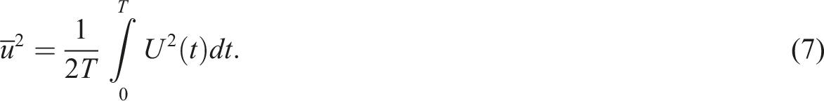
The proposed solution (8) encompasses a singular unknown, specifically the frequency ω, which necessitates determination. Substituting (8) into (7) results in

By inserting (9) into (6), the frequency is ascertained as suggested by He.33,67,68 Additionally, He
42
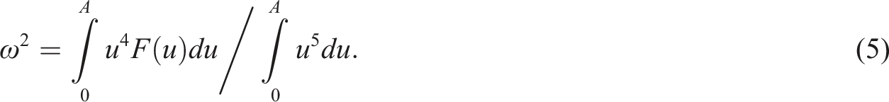
defined the frequency of the cubic oscillator as comparable to the function’s first derivative concerning the variable u evaluated at the designated point

Recently, El-Dib39,71 presented an improved formulation of the stiffness term for the nonlinear equation (3), as illustrated below

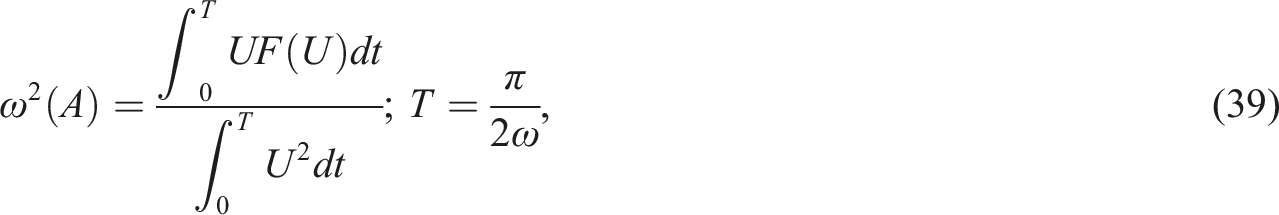
Then, independently integrate the numerator and denominator of the stiffens term related to the variable t from zero to T where T is the period. When compared to equation (4), the formula of the frequency will take the following shape
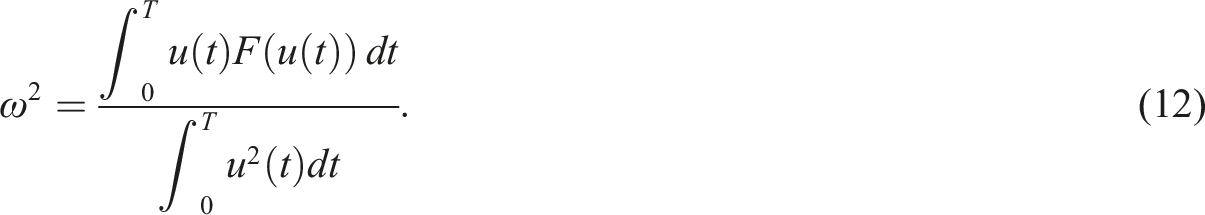
The above formula can be established using the mean square error technology:
The following error was made while comparing equation (4) to equation (1)

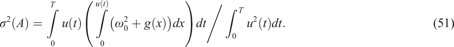
The mean square error is defined as

The minimum value requires that


The result of solving equation (16) is formula (12). The frequency corresponding to the appropriate trial solution that matches the initial conditions can be obtained by performing the aforementioned integrals. The benefit of using this formulation is that it enables analysis of the frequency for successive approximations to the generalized Duffing oscillator. The formula presented above offers the most efficient and straightforward method for calculating frequency. The analysis procedure described above validates the frequency formula’s accuracy.
Enhanced He’s frequency formula
We shall explain how He’s frequency formula (6) can be included in El-Dib’s frequency formula (12) in the paragraphs that follow:
Let’s define the function

Consequently, the generalized form of equation (1) is represented as

The linear harmonic equation is discovered if n = 0 in equation (18), and its potential frequency calculated as


The cubic Duffing’s frequency in this instance has been proved by He
33
to correspond to the first derivative of the function

Utilizing

To estimate the frequency

This outcome perfectly matches He’s
69
observations. It does not, however, precisely match the results obtained from the sophisticated Lindstedt–Poincaré solution.
66
The frequency-amplitude connection is found to be as follows in Ref.
72

Consequently, relying solely on the first derivative for

Furthermore,

Once more, the frequency estimation, when derived through the derivative

This result is not in concordance with the findings derived from the Homotopy Perturbation Method (HPM)
66
nor with those from the equivalent linearized method
73

As previously highlighted, the appropriate derivative methodology is

For elevated values of n, the precise derivative formula to determine the frequency can be expressed as
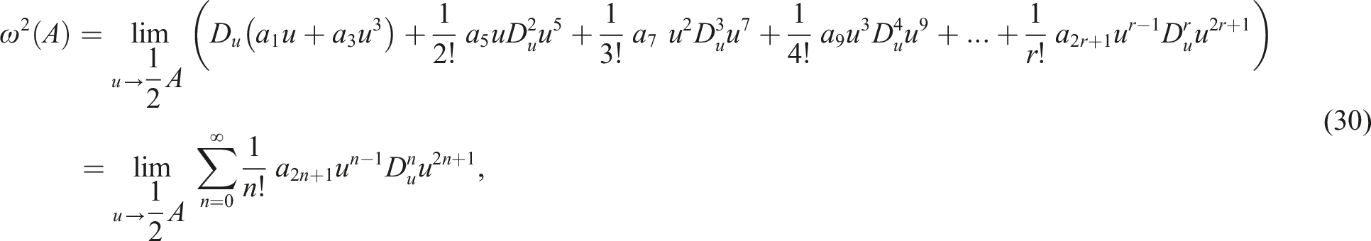
This is a development of He’s fundamental frequency formula, where
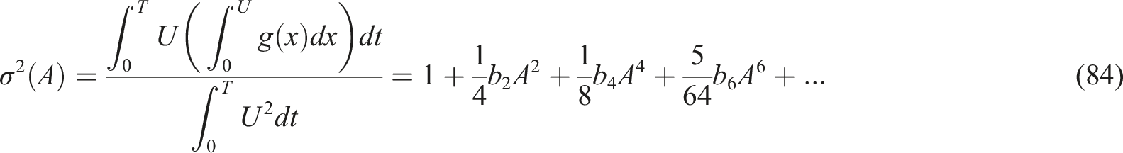
Frequency formula in terms of a power series form
When the infinite series (30), which results in, is expanded, the significance of this frequency may be appreciated

The series given above can be formatted as a power series as
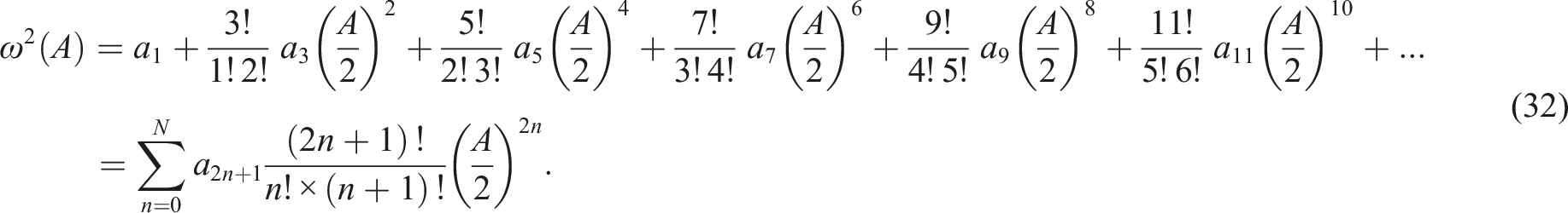
This suggests that the interrelation between frequency and amplitude has been examined through the lens of a power series, consistent with the differential expression depicted in (30).
It’s important to note that the nonlinear equation (18) can be simplified to the form of a fundamental pendulum equation if the coefficient

Using (32) as a starting point, the corresponding linearized form is

This suggests that the frequency articulating the simple pendulum’s oscillation is as follows

This aligns with the findings previously reported in Ref.
24
The following format can be used to indicate a rough solution

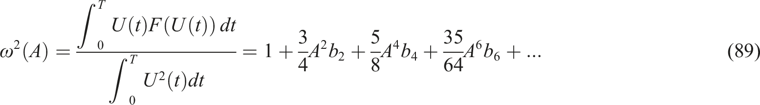
The integrative performance of the frequency formula
Utilizing the expansion denoted by (31) is beneficial for calculating the frequency for higher values of n in the generalized
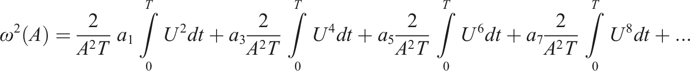
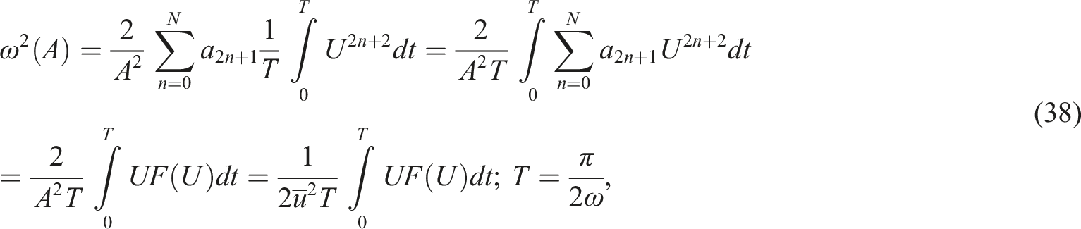
For a generic trial solution, the aforementioned formula can be represented in the format of (12).
To elucidate the precision of the solution using formula (12), one might examine the Duffing oscillator characterized by cubic nonlinearity

Deriving the analytical solution can be expressed as The visualization of the approximate solution to equation (40) for 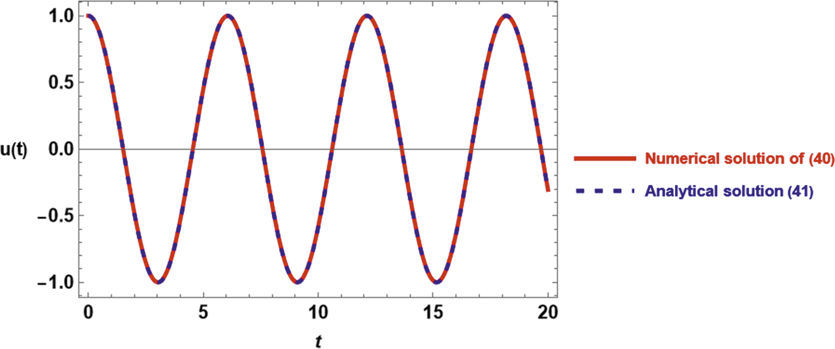

This comparison shows that the analytical solution has an excellent agreement with the numerical solution.
The Helmholtz oscillator
The Helmholtz oscillator has garnered significant attention from the scientific community, as evidenced by the extensive body of research on the topic. 73 Recognized as a foundational principle in both physics and engineering, the Helmholtz oscillator has been the focal point of myriad scholarly inquiries. 74 Over the past decade, the nonlinear Helmholtz equation has been a particular area of emphasis. The practice of translating real-world challenges into mathematical models serves as a potent instrument for comprehension. It is posited that solutions derived from these models can offer insights into the dynamics of nonlinear oscillations across various scientific and engineering domains, including but not limited to, electronics, naval applications, finance, and other models. 75 This manuscript introduces an analytical method tailored for crafting the frequency formula pertinent to the Helmholtz oscillator. Helmholtz-type nonlinearities, characterized by quadratic characteristics, owe their nomenclature to Helmholtz’s pioneering assertion that the eardrum functions akin to a linear and quadratic geometric component-based restoring force to an asymmetric oscillator. 76 Contemporary research, however, has shifted its focus towards non-perturbative approaches in the pursuit of optimal approximate solutions. 37
Established the frequency formula for the quadratically nonlinear oscillator
When the function


Let’s assume that the initial condition remains valid. If we posit that equation (42) possesses a precise direct frequency formula


It’s important to highlight that when the function
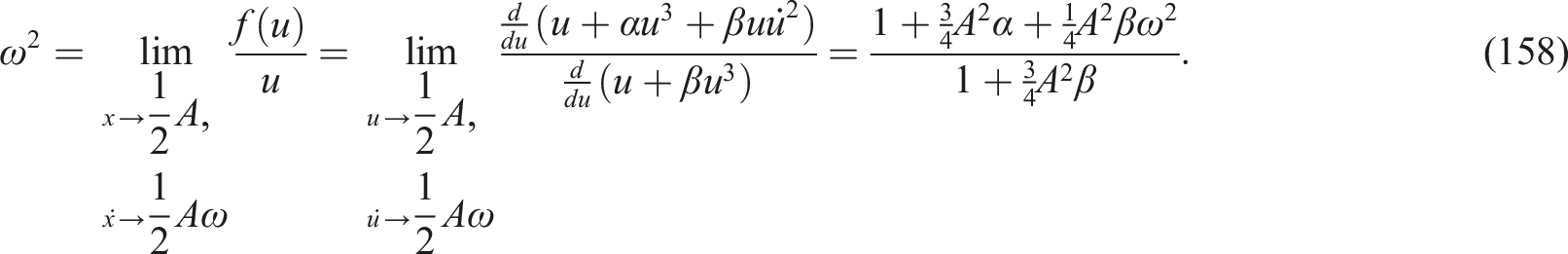
Given that an even function can be derived from the differentiation of an odd function concerning the variable u, the even function

Differentiating the power series (17) concerned with the variable u gives


It should be observed that the corresponding differentiative form

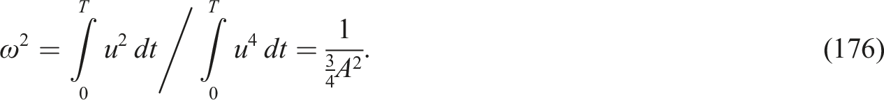
To derive the integrative form of the parameter

Employing (50) with the integrative frequency formula given in (39) yields
To illustrate this objective, the solution for the quadratically nonlinear oscillator, as represented by (42), can be expressed as follows

The frequency

The frequency

To ascertain the accuracy of the suggested approach, a numerical solution is employed as a reference point. A side-by-side comparison with the numerical solution of equation (53) is undertaken to assess the solution given by equation (52). The outcomes are showcased in Figure 2. The exact numerical solution of equation (53) is represented by a solid red line, whereas the blue-dashed line signifies the analytical solution (52). This juxtaposition underscores the accuracy of the analytical solution provided by (52). The visualization of the approximate solution to equation (53) for 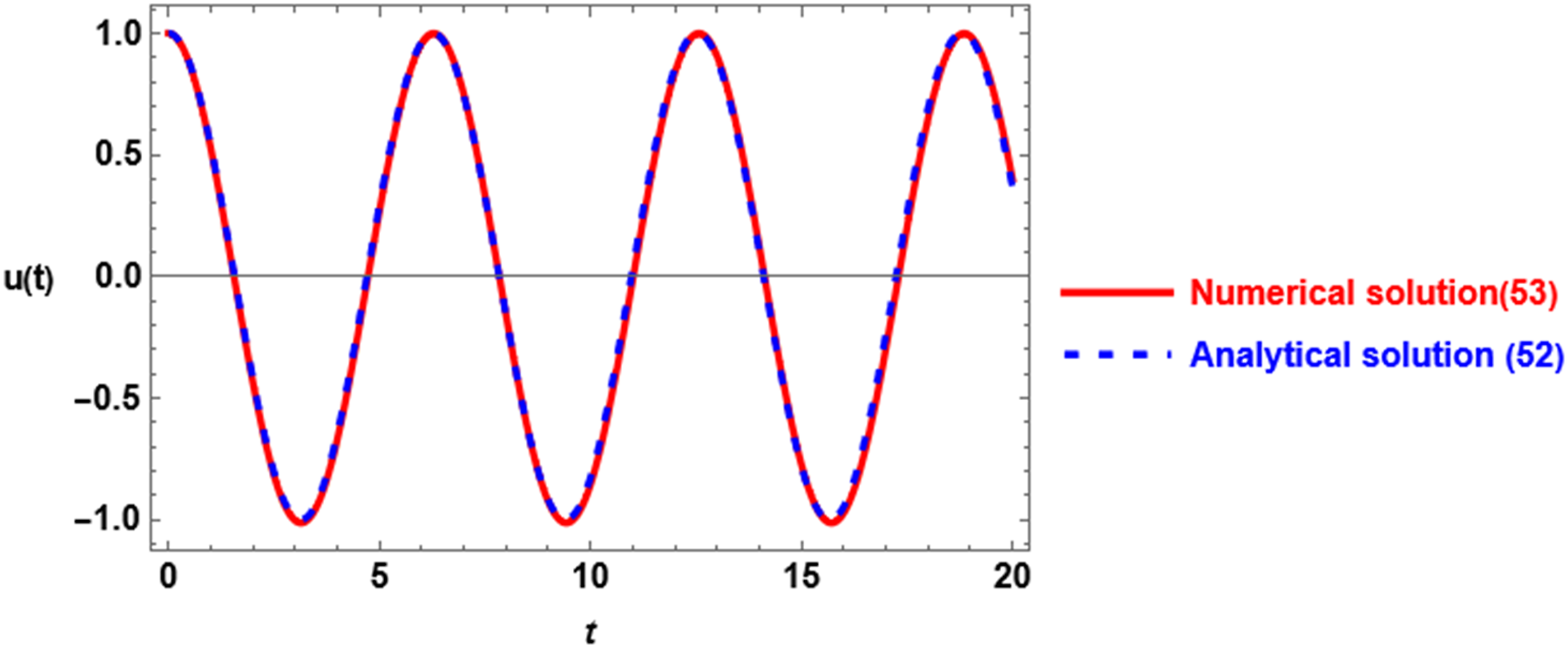
Frequency formula for the Helmholtz–Duffing oscillator
An oscillator where the restoring force is not confined solely to odd functions or exclusively to even powers, but encompasses both odd and even powers, is termed the Helmholtz–Duffing oscillator, as illustrated below

The functions


A straightforward methodology to derive the linearized version of an oscillator (55) can be articulated using El-Dib’s formula (12). This can be accomplished by reformatting equation (55) into the subsequent alternative expression
61

Accordingly, equation (60) will linearized in the form

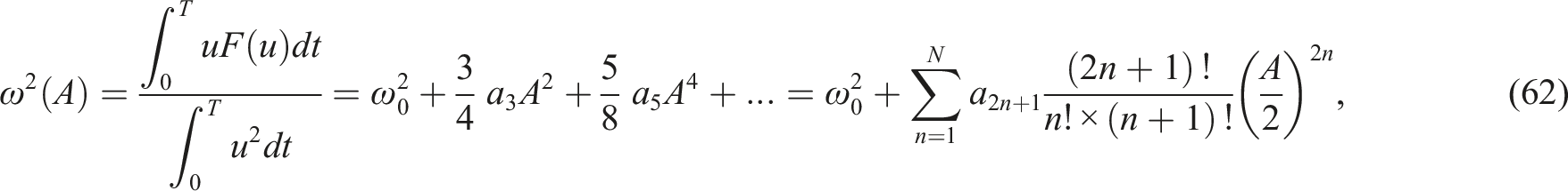
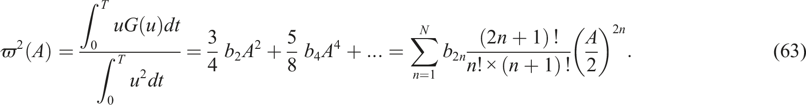

Figure 3 showcases a comparison between the analytical solution of equation (55) and its numerical counterpart. Both the analytical solutions, denoted by (59) and (64), will be juxtaposed for evaluation. For this illustration, we will consider specific functions, accompanied by the initial conditions set out in (2)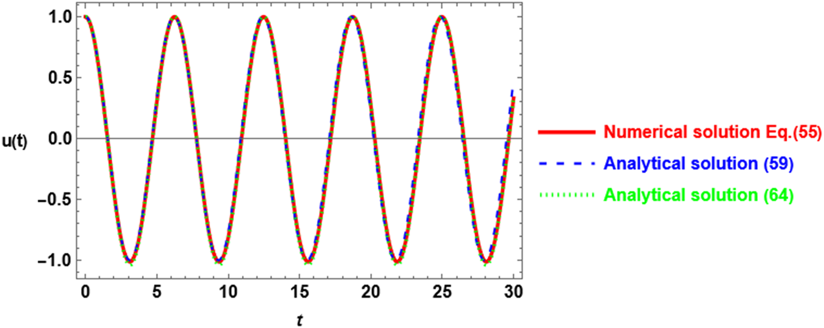


The frequency corresponding to solution (59) is defined as

The frequency associated with solution (64) and the value of the non-homogeneous component are, respectively, provided by


The analytical solutions, as denoted by (59) and (64), are graphically represented alongside the numerical solution of equation (55) in Figure 3. The approximate solution, as outlined by (59), is depicted by a blue-dashed line, whereas the analytical solution (64) is shown with a green-dotted line. In contrast, the numerical solution corresponding to the Helmholtz–Duffing equation (55) is marked by a red solid line, specifically for a system characterized by parameters
Application
The application focuses on a general vibratory system about N/MEMS, elucidating the theory outlined in the preceding formalism.
Consider the dynamics of microstructures, which can be depicted by a nonlinear ordinary differential equation. This equation embodies the typical form associated with a set of oscillators from N/MEMS,76–79 commonly employed in the realms of nanoscience and nanotechnology

Given the initial conditions:
Equation (70) serves as an extension of the Helmholtz–Duffing oscillator, which is composed of a combination of both odd and even nonlinear terms. It can be expressed as


Equation (71) can be reformulated as
48

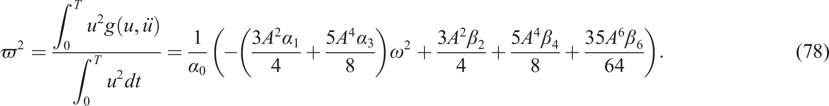
By integrating both the numerator and the denominator independently over the interval (0, T), we get
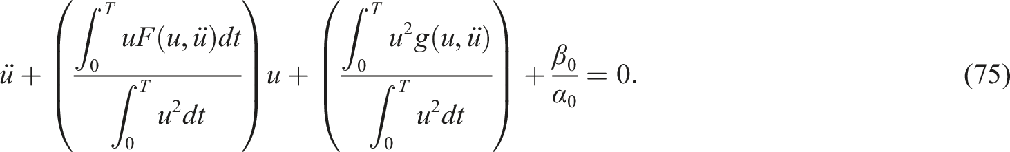
By utilizing the trial solution given in (8) and proceeding with the integration, equation (75) can be reformulated as

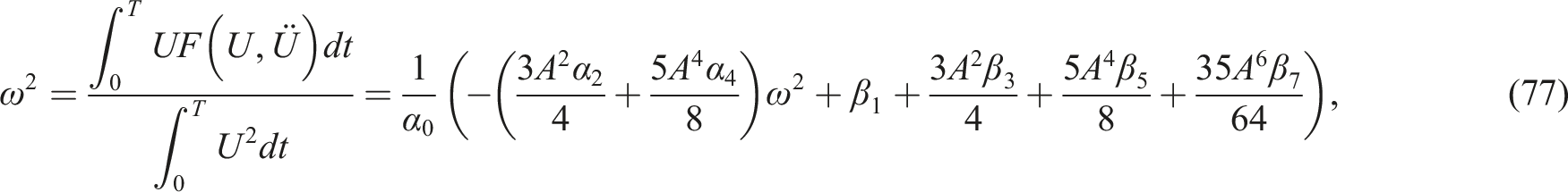
Solving equation (77) for
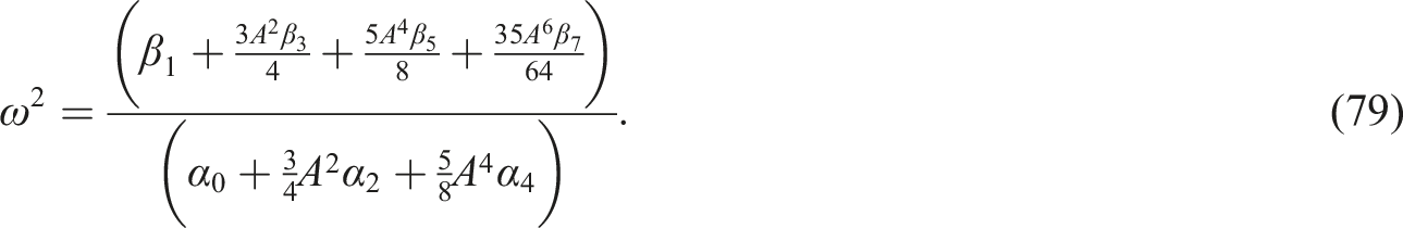
The solution of the non-homogenous second-order harmonic equation (76) is given by

The solution is visually represented in Figure 4, juxtaposed with the numerical solution for equation (70). A scrutiny of Figure 4 reveals that the analytical solution aligns exceptionally well with the numerical counterpart, showing a relative error estimated to be 0.027. Comparison of the approximate solution 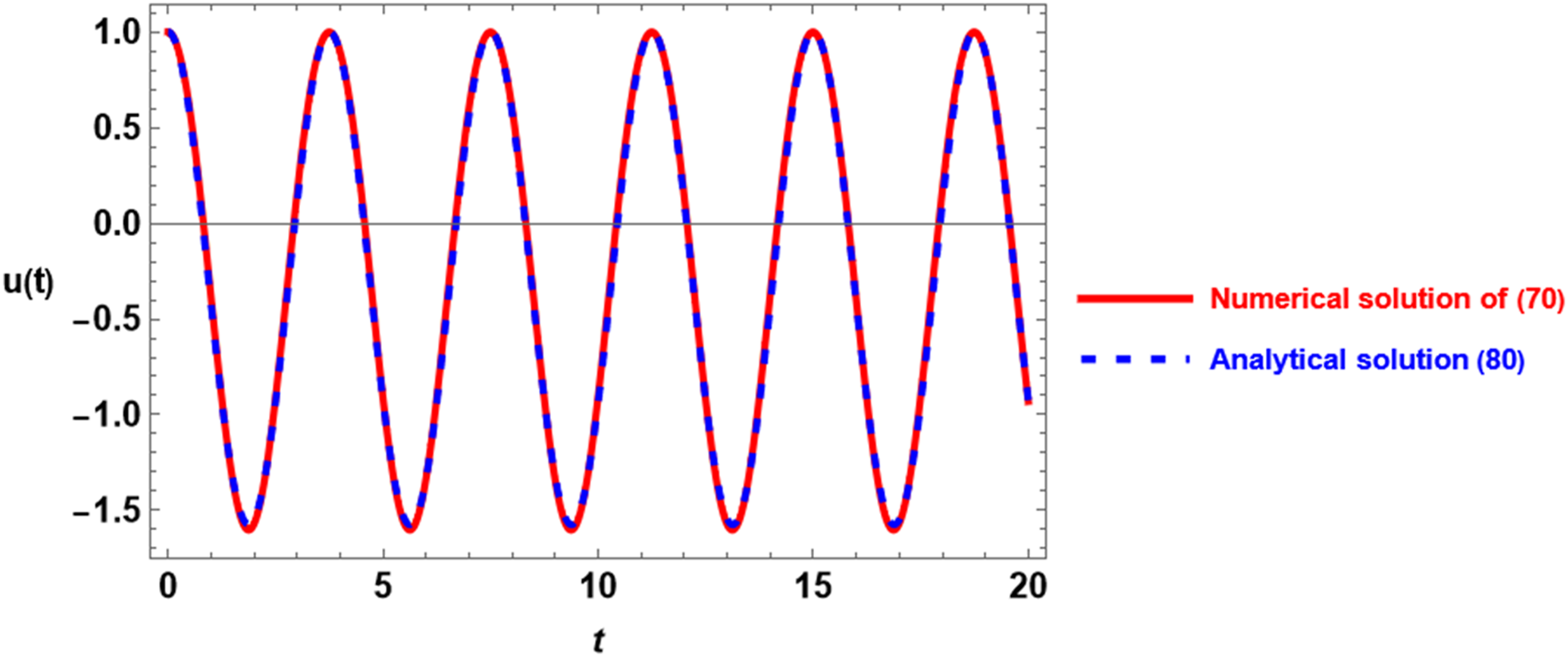
The Van der Pol oscillator, augmented with extended damping nonlinearity
Van der Pol is celebrated for the eponymous equation that delineates a rudimentary self-oscillating triode circuit. 80 This equation has been the cornerstone for a myriad of electro-technical apparatuses, where the triode is replaced with entities like an arc lamp, a glow discharge tube, or an electronic vacuum tube. When augmented with a driving term, this equation stands as a benchmark system manifesting chaotic dynamics. Moreover, it’s associated with a prominent class of oscillations termed relaxation oscillations. Here, “relaxation” refers to the discharging activity of a capacitor. Van der Pol played a pivotal role in championing this nomenclature, which is deeply rooted in the nascent stages of nonlinear oscillation theory. 81
Van der Pol has demonstrated a dissipative equation that exhibits prolonged spontaneous oscillations without the use of force. The equation describing the amplitude of an oscillating current produced by a triode can be streamlined as follows
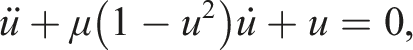
In the ensuing section, our focus will be on the Van der Pol oscillator, with a particular emphasis on damping forces that incorporate higher-order nonlinearity. The goal is to distill this oscillator down to a fundamental harmonic oscillator. Drawing from the knowledge accumulated in our previous deliberations, we aim to refine the quadratic order of nonlinear forces.
Suppose we have a Van der Pol oscillator given in the form


It’s important to highlight that the initial conditions, as denoted by (2), remain applicable. The primary objective is to linearize this oscillator. It’s observed that the damping force’s nonlinearity manifests in a quadratic form. The fundamental principle revolves around transforming squared powers into odd powers. This transformation can be achieved in one of two methods. Firstly, it’s recognized that odd powers can be derived by integrating the quadratic powers related to the variable u. Subsequently, one can utilize formula (51) to derive a constant damping term. The alternative approach involves expressing these powers as a rational fraction. This is done by multiplying the numerator with the variable u and then dividing by the same variable. Consequently, both the numerator and denominator evolve into odd functions. In such scenarios, the El-Dib integral formula, denoted by (12), becomes applicable. This formula yields a constant that symbolizes a function in terms of amplitude A. The result is a straightforward harmonic equation.
Accordingly, the first scope of the nonlinear oscillator (81) can be rewritten in the form

The damping linear oscillator (83) has the following solution
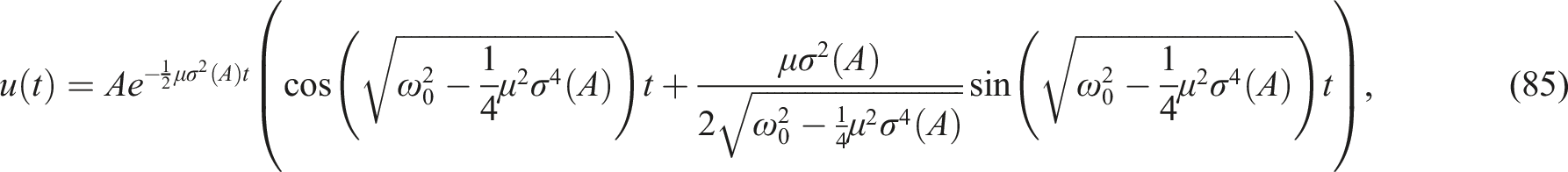
Given the second scope, equation (81) can be reformulated as


Employing the trial solution (8) and using the El-Dib formula (12) to the above equation which is reduced to

As mentioned before, the solution of equation (88) can be written as
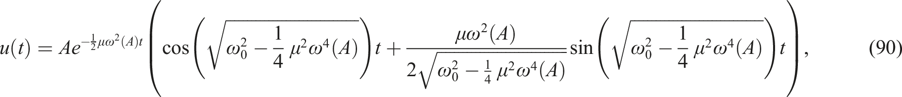
To shed light on the analytical solutions of equation (81), we undertook a numerical comparison of solutions (85) and (90) against the numerical solution of equation (81), as previously delineated. By consolidating the numerical representations of these three solutions into one unified format, we aimed to simplify the comparative analysis and pinpoint the most precise solutions. The graphical representation reveals a commendable alignment of both solutions with their numerical counterpart. Figure 5 Specifically, the relative error for solution (85) stands at 0.02601, while the error associated with solution (90) is measured at 0.06954.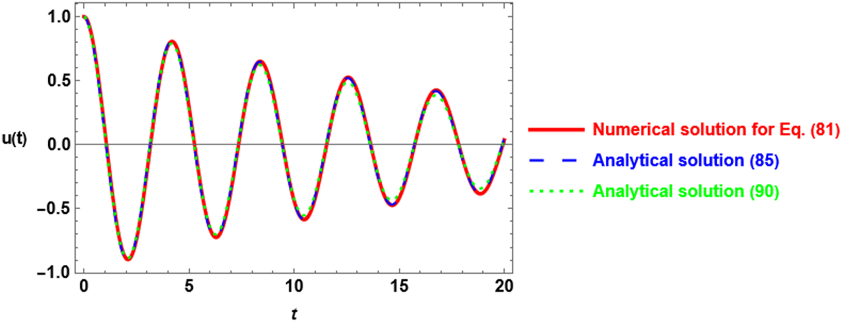
with the numerical solution of equation (81) for a system of
Fast and simple approach to establish the equivalent linearization oscillation
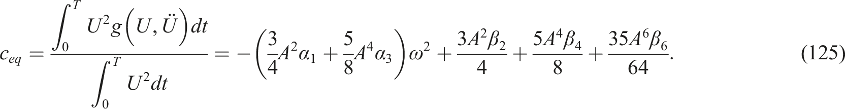
In the present section, our focus is on broadening the application of the El-Dib formula (12) to address oscillators exhibiting pronounced nonlinearity. The fundamental premise of El-Dib’s approach operates as follows:
Suppose we possess a function represented by a differential equation. This function exhibits nonlinearity of the variable u and includes both its second and first derivatives concerning the independent variable t, presented in the format

The target is to discern how to derive an equivalent linear differential equation from the nonlinear version, characterized as follows


The comparison of equations (92) and (94), leads to express the following errors

The total mean square errors are convenient to use here, which are defined as
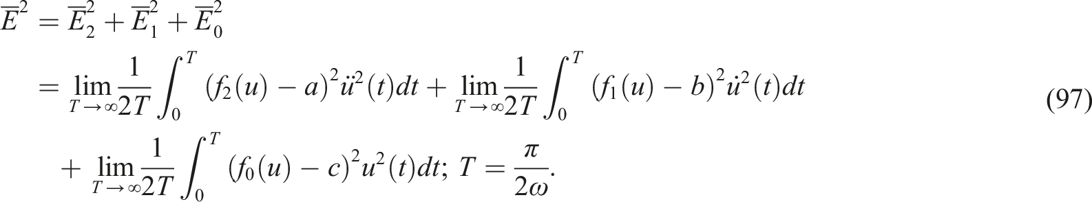
The minimum value requires that


Upon simplification, we arrive at the subsequent equations


To derive the equivalent linear second-order differential equation using the conventional derivative, one must introduce the trial solution U that adheres to the initial conditions specified for the problem at hand. By aptly selecting the trial solution, the corresponding approximate solution can be achieved. Moreover, the aforementioned formulas can be employed to generate successive approximate solutions, as detailed in Ref. 82
Let’s assume we possess a series of trial solutions for the nonlinear oscillation: U0(t), U1 (t), U2 (t), …, and so forth. These are denoted as the zero-order, first-order, second-order, and subsequent orders of approximate solutions. For each instance, there are distinct coefficients corresponding to the order of the approximate solution. Consequently, the linear equation (92) transforms into


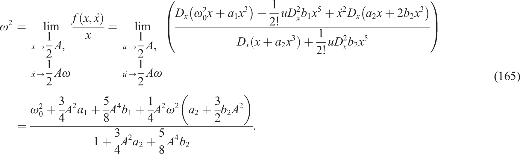
Assuming the partial derivatives provided in equation (95) are expressed in terms of the trial solution

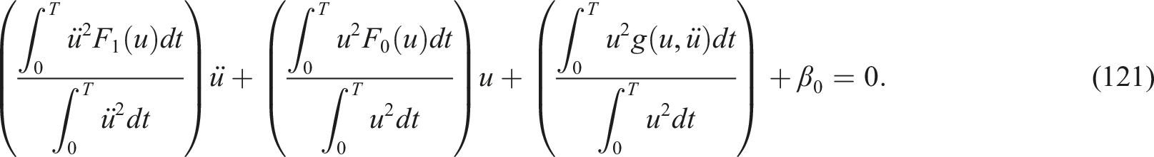
Employing (108) into equation (94) which can be rearranged as

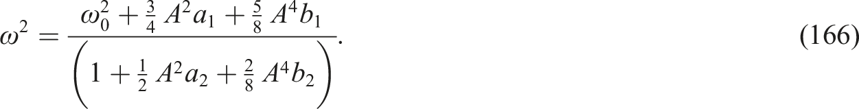
By integrating both the numerator and the denominator for each coefficient of the aforementioned second-order equation across the domain
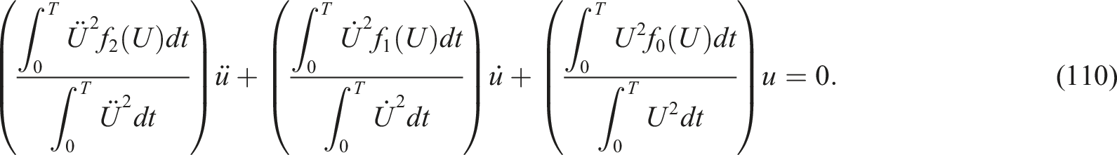
This can be rewritten in the familiar situation of the damping linear second-order equation as follows


The linear damping equation, represented by (111), possesses a solution in the format


Application
One can apply the formula presented in equation (110) to the example outlined in equation (70). It’s evident that this equation is formulated as


Utilizing El-Dib’s enhancement,
40
equation (116) can be restructured as

Applying the integral form yields
By utilizing the trial solution given in (8) and completing the integrations, the linearized version corresponding to the original equation (116) is derived as

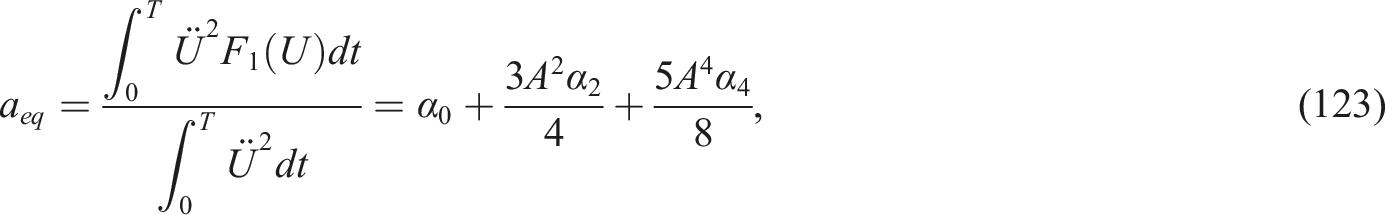
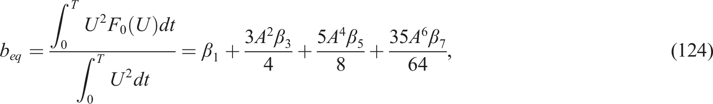


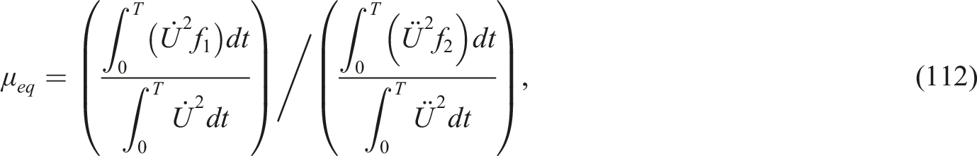
From (124) and (123), it’s evident that the frequency
Implementation of the Toda oscillator
The Toda oscillator is a well-known nonlinear system that arises from the Toda lattice, a one-dimensional chain of particles with an exponential interaction potential. The Toda lattice and its associated oscillator have been studied extensively due to their integrable nature and the presence of soliton solutions. The Toda oscillator and lattice have applications in various fields, including condensed matter physics, nonlinear optics, and even biology. The integrable nature of the system makes it a valuable tool for studying more complex, non-integrable systems.
This example is dedicated to providing a concise overview of the Toda oscillator as referenced in Refs66,83,84

It’s advantageous to bifurcate the nonlinearity into odd and even nonlinear forces. Substituting the exponential function in equation (80) with its counterparts, the hyperbolic functions

Selecting

Equation (129), when expressed in terms of the Taylor expansion, can be represented in the form of a power series. This utilizes expansion (32) for the odd function and expansion (48) for the even function.
The Toda oscillator will have the form if the coefficient


This is the equivalent linearized form of the Toda oscillator given by equation (128), which has the following solution

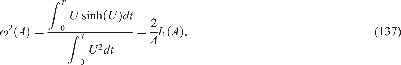
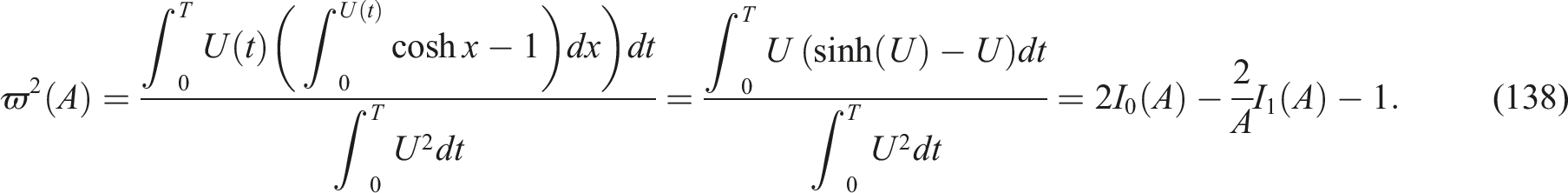
El-Dib’s formula (12) can be used to derive the previously indicated solution. Equation (129) can be rewritten as

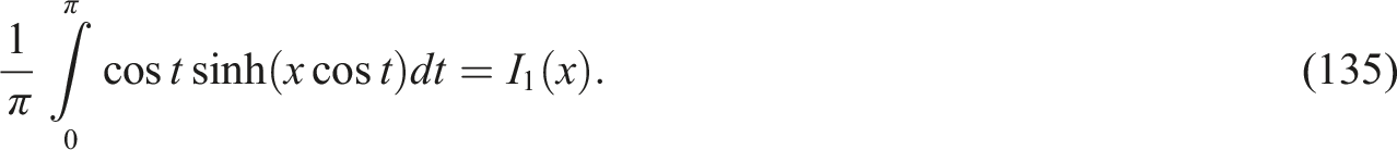
Utilizing the trial solution given by equation (8), integrate the denominators of the two fractions across the time interval (0, T), as well as the numerators. The resulting integral representation of the first kind of Bessel functions can be expressed as
Equation (134) transformed to the linearized form

The Toda oscillator is a rich and complex nonlinear system that offers a plethora of interesting dynamics and behaviors. Its study can provide valuable insights into the general nature of nonlinear oscillatory systems and their associated phenomena. Figure 6 shows the numerical representation of Toda’s frequency formula. The comparison with the numerical solution demonstrates that the analytic periodic solution (133), represented by the blue-dot-curve, and the numerical solution, represented by the red-dash-curve, have a good agreement.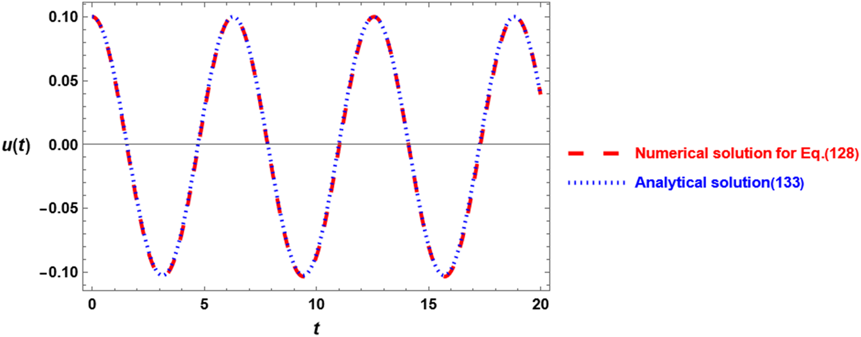
Implementing the Tangent (or hyperbolic tangent) oscillator
The Tangent (hyperbolic tangent) oscillator is a specific type of nonlinear oscillator that involves the tangent function in its formulation. To implement or analyze the Tangent oscillator, one would typically start by defining its differential equation and then proceed to solve it using various methods. For a small amplitude of oscillation, you might be able to use perturbation methods to find an approximate solution. For larger amplitudes or more complex scenarios, numerical methods method might be more appropriate. Here’s a general analytical non-perturbative approach to implementing the Tangent oscillator:
The oscillator characterized by the tangent function is presented as85,86

It makes sense to assume that the weighted residuals methodology and the frequency formula of He, which are two different approaches that can be used to determine the frequency formula for the nonlinear oscillator, would yield consistent results. The frequency formula of He is specifically used in
86
for the odd function and is described as follows

As was previously established, the frequency extracted from the aforementioned peculiar non-polynomial function is not accurate. It is well-known that if the function isn’t expanded, the implementation of Galerkin’s integral formula is impractical. The methods presented in this study can be used to derive a more accurate frequency formula. When the function is replaced with the hyperbolic tangent, the oscillator takes on the subsequent form, as detailed in reference
87

Equation (141) can be reformulated as

Considering the fraction in the preceding equation, which features an odd numerator and an even denominator, one can expect this equation to be transformed into the subsequent linear form

To evaluate both the numerator and the denominator of equation (143), one can restructure equation (142) in the following manner

Applying the integrative approach for the numerator as well as the denominator should be treated separately, as follows
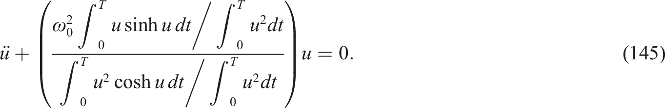
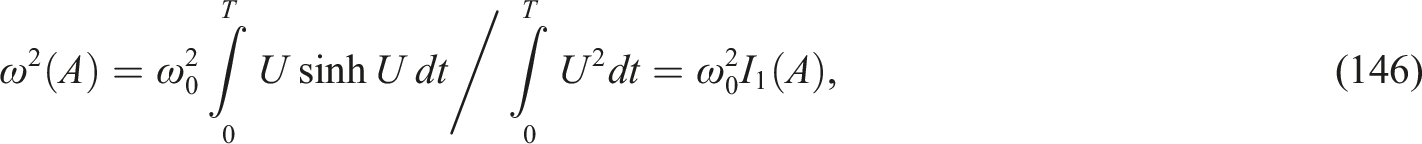

Accordingly, equation (145) becomes

Its solution seeking in the form
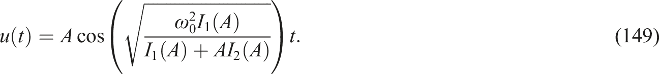
Should the function
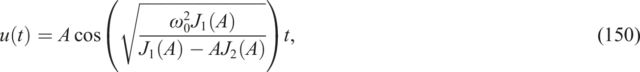
Once we have a solution, we can analyze it to understand the behavior of the Tangent oscillator. This might involve plotting u(t) versus time. Fig.(7) illustrates a comparison between the analytical solutions outlined in equation (149) and the precise numerical solution corresponding to equation (141). This visualization spans various amplitude values to facilitate a comprehensive comparison. Significantly, the solution delineated by equation (149) aligns impressively with the numerical solution across the entire amplitude spectrum.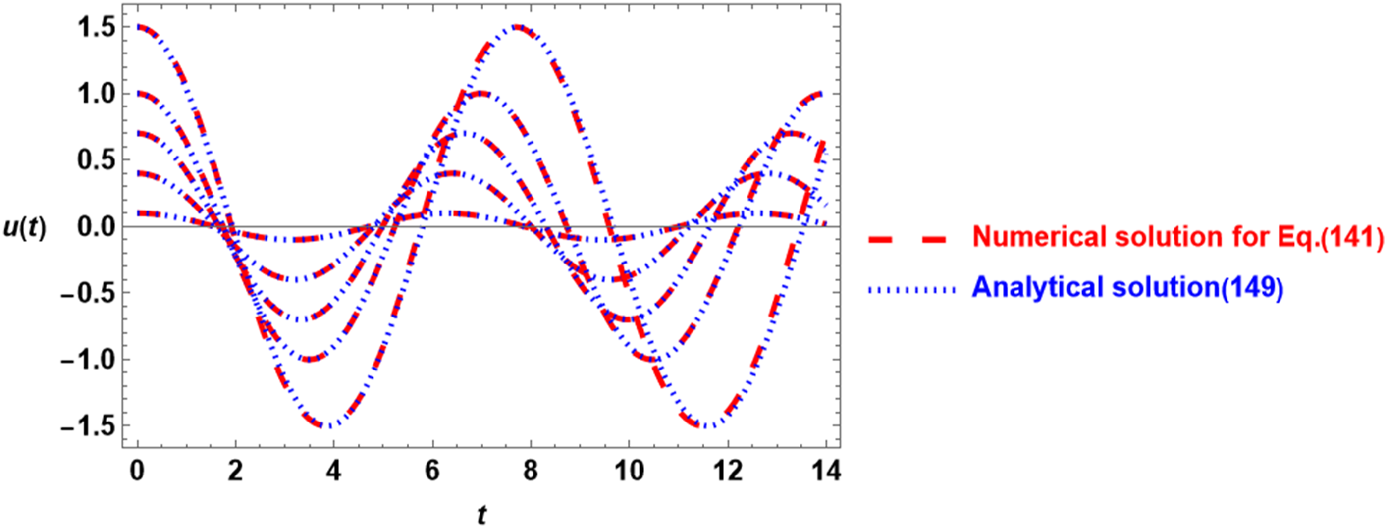
Relative restoring forces oscillators
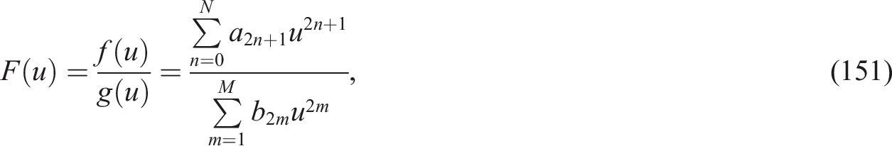
Oscillators with relative restoring forces are a subset of nonlinear oscillators where the restoring force is not just a function of the displacement but also depends on a fractional composed of two parts of a numerator function and another denominator function in variables of the system. The behavior of oscillators with relative restoring forces can be quite complex due to the interplay between the various terms. They can exhibit a range of behaviors, from simple periodic motion to chaotic dynamics.
This section explores nonlinear oscillators characterized by an even denominator present within the odd numerator of the restoring force. The literature has presented various restoring forces characterized by an even denominator. For an oscillator with a specific relative restoring force, it can be expressed as
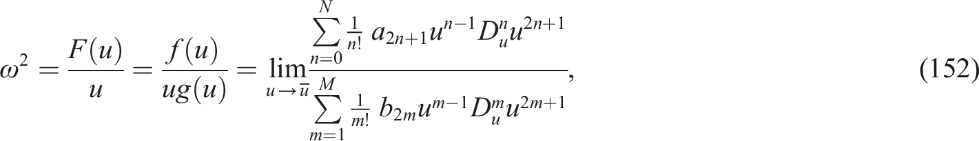
Utilizing the expanded He’s frequency formula (30), the frequency can be determined in the following manner

Application to vibration mode of a tapered beam
The vibration of tapered beams is a topic of interest in structural dynamics and engineering. Tapered beams, unlike uniform beams, have a non-constant cross-sectional area along their length. This variation in cross-sectional area introduces complexities in the vibration behavior of the beam. The following mathematical expression describes the principal vibrational formula of a tapered beam as mentioned in Ref
88


To linearize the above nonlinear equation, one can employ the modified He’s formula (30). By doing so, the nonlinear terms can be approximated, and the equation can be transformed into a linear form. This linearized equation can then be solved using standard techniques to obtain the vibration mode shapes and frequencies of the tapered beam. Upon applying the modified He’s formula (30), the vibration characteristics of the tapered beam can be determined. 89 These characteristics, such as the natural frequencies and mode shapes, are crucial for design and analysis purposes. 90
It is possible to rewrite this oscillator as


Since the odd numerator is present, the frequency can be roughly expressed as follows
As a result, the frequency is expressed in the format

We arrive at the same frequency formula by using Galerkin’s approach and the trial solution (8), which is presented as

The rough answer to equation (154) is as follows

It’s worth noting that the results obtained using He’s formula should be validated against experimental data or numerical simulations to ensure accuracy. 91 In conclusion, the application of He’s formula (30) to the vibration analysis of tapered beams provides a simplified approach to understanding their dynamic behavior. This method offers a quick and efficient way to analyze such complex structures without delving deep into intricate numerical simulations.
The free vibrations with type fifth-order nonlinearities 92
The fifth-order nonlinearities introduce additional complexities to the vibration behavior of the oscillator. Such nonlinearities can arise in various physical systems, especially when the amplitude of vibration becomes large.
Mathematical representation for the differential equation representing the free vibrations of a conservative oscillator with fifth-order nonlinearities is expressed by

To analyze the system, one could employ techniques like the modified He’s formula (30), which has been discussed earlier. This would involve approximating the fifth-order term to transform the equation into a more tractable form. Once linearized, standard techniques can be used to determine the system’s response. Solving the linearized equation will provide insights into the vibration characteristics of the oscillator.
Equation (162) can be rearranged as follows

This leads to the following formulation of the regaining force

Hence, the frequency is determined to be
Upon further simplification, the frequency is deduced as
By opting for the suggested solution (8) as previously indicated, the frequency derived from the Galerkin formula takes the shape


However, it’s essential to remember that the linearized solution is an approximation that becomes significant

The simplest way to find nonlinear singular oscillator frequency
The frequency of nonlinear singular oscillators is of importance in the field of nonlinear dynamics. 93 Singular oscillator equations of motion contain terms that, under certain conditions, become unbounded, or infinite. 93 Determining the frequency of such oscillators is challenging due to their singularities. 94 Since singularities might lead to infinite reactions, several traditional methods are not suitable. The frequency may vary in tandem with the amplitude, especially in highly nonlinear systems.
Finding the nonlinear singular oscillator’s frequency is the main goal of this section. We shall look at the single oscillator’s frequency-amplitude connection. Connecting the frequency and amplitude of nonlinear oscillators is one way to use this technology. It may be necessary to modify the conventional method for singular oscillators in order to accommodate the singularities.
For the special attention to the oscillator
Although there are various approaches to finding the frequency of nonlinear singular oscillators, the best approach for a given system often depends on its particular features, such as its singularity and nonlinearity. Examine the system below that exhibits strong singularity as

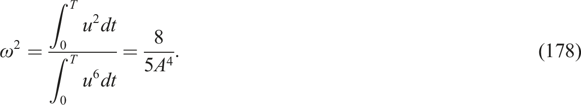
Applying He’s frequency formula directly yields the following frequency calculation

This result makes ω imaginary and shows that there is no oscillation. The distinctive development of the restorative force

One interesting word for the restorative energy shown in (172) is the enhancement of the original function. The frequency is determined directly from the original potential function; the enhancement technique is solely needed to produce an odd numerator and an even denominator. Taking (172) as a ballpark estimate for the frequency, we arrive at

Combining (172) and (173) yields a valid formula with two odd polynomials in the numerator and denominator. As such, He’s differentiative technique will be applied separately to the numerator and denominator. The frequency is then determined to be

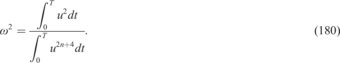
Equation (170) can be rewritten to adapt the integrative frequency formula to the particular requirements and characteristics of the nonlinear system being studied

Interestingly, the outcomes of this approach agree with the results of using He’s formula. This congruence demonstrates the effectiveness of the proposed method in solving special issues in nonlinear oscillatory systems. In addition to confirming the methodology, the consistency of the results confirms El-Dib’s frequency formula (12) as a trustworthy analytical tool. This type of connection is significant because it demonstrates how multiple analytical methods can converge to provide comparable outcomes. This boosts confidence in the theoretical understanding and practical implementation of these strategies in the handling of difficult dynamic problems.
Remark: for the anti-cubic nonlinearity


The stronger restorative force is
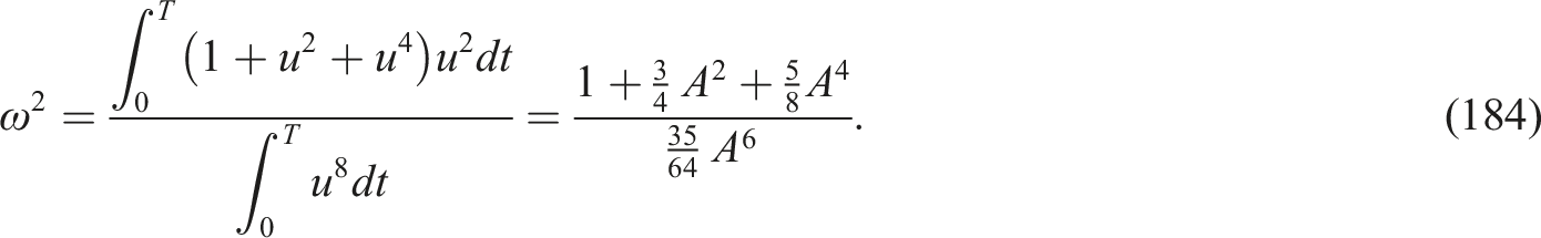
Examine the singular oscillator composed of anti-cubic and anti-quintic equations that follow

It is convenient to rewrite equation (181) in the form

The improved restorative force has the following format

Hence, the following is a representation of the approximate solution

Examine this Duffing using an Anti-Cubic Oscillator

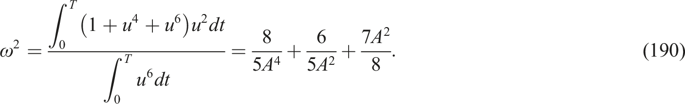
There are two distinct parts to the restorative force


Enhancing the restoring force as

The frequency can therefore be calculated as
The following form of the solution is identified
Conclusion
This study presents refined methodologies adept at formulating periodic solutions for the generalized Duffing and Helmholtz oscillators, as well as their related variants. The nonlinear facets of the oscillator are categorized into distinct odd and even components. Both these components play pivotal roles in shaping the frequency. Notably, the even components necessitate integration concerning the system variable for frequency determination. Collectively, they can be synthesized to craft a non-homogeneous linear harmonic equation. The oscillator’s frequency is discerned from the secular function, which embodies the odd component. In contrast, the non-secular function, representing the even component, aids in elucidating the non-homogeneity of the harmonic oscillator. This strategy culminates in three unique nonlinear frequency styles and their corresponding inhomogeneity components. The frequency, in its differential guise, is showcased as an extension of He’s formula. Simultaneously, a frequency rendition in the vein of a power series is elucidated. Moreover, a frequency interpretation in an integrative mold is also delineated. This technique finds applicability in the Toda, Tangent, and Van der Pol oscillators. The proposition’s scope is further expanded to encapsulate the singular oscillator. In the realms of engineering and science, it’s commonplace to encounter even functions, quadratic forms, or singularities. This research augments the guidance on the utilization of frequency formulas for all-encompassing nonlinear oscillators. It’s imperative to underscore that the El-Dib frequency integrative formula, encapsulated in equation (12), epitomizes the most streamlined articulation of the amplitude-frequency relationship. As the saying goes, “In nonlinear vibration theory, elegance lies in simplicity.” This manuscript proffers a potentially streamlined methodology for the expeditious evaluation of a nonlinear oscillator’s frequency attributes. The outcome of this singular approach is laudably precise, underscoring its commendable accuracy.
Future directions in this research area will focus on several key aspects. Firstly, there will be a continued emphasis on refining and enhancing the present approach, particularly in terms of the advanced trial solution. This will involve developing more accurate approximations and incorporating additional factors to improve the precision of the analytical solutions obtained. Furthermore, there will be a concerted effort to address the discussion of the solution in the presence of the periodic force. This entails exploring the effects of the periodic force on the stability and dynamics of the system in greater detail. Additionally, there will be a focus on understanding how various parameters, such as the amplitude and frequency of the periodic force, influence the behavior of the system, and its response to external stimuli. Overall, future research endeavors will seek to deepen our understanding of nonlinear oscillatory systems and their responses to external forces. By refining analytical techniques and exploring the effects of different factors on system dynamics, researchers aim to provide valuable insights into the behavior of these complex systems and pave the way for advancements in various fields of science and engineering.
Footnotes
Author contributions
The author is solely responsible for the conception, formulation, derivation, calculation, drafting, revision, and submission of the paper.
Declaration of conflicting interests
The author(s) declared no potential conflicts of interest with respect to the research, authorship, and/or publication of this article.
Funding
The author(s) received no financial support for the research, authorship, and/or publication of this article.