
Abstract
In this paper, the Khater II analytical technique is used to examine novel soliton structures for the fractional nonlinear third-order Schrödinger (3-FNLS) problem. The 3-FNLS equation explains the dynamical behavior of a system’s quantum aspects and ultra-short optical fiber pulses. Additionally, it determines the wave function of a quantum mechanical system in which atomic particles behave similarly to waves. For example, electrons, like light waves, exhibit diffraction patterns when passing through a double slit. As a result, it was fair to suppose that a wave equation could adequately describe atomic particle behavior. The correctness of the solutions is determined by comparing the analytical answers obtained with the numerical solutions and determining the absolute error. The trigonometric Quintic B-spline numerical (TQBS) technique is used based on the computed required criteria. Analytical and numerical solutions are represented in a variety of graphs. The strength and efficacy of the approaches used are evaluated.
Keywords
AMS classification: 35J10; 35D30; 35R10; 65N15; 35Q51
Introduction
Numerous academics in diverse fields, including engineering and applied sciences, have recently concentrated their efforts on the physical interpretation of optical fibers. 1 Organic artificial materials used in the manufacturing of optical fibers include the well-known silica (drawing glass) and polymers with a thickness less than a human hair. 2 This procedure transforms the fiber into a translucent one with increased flexibility. 3 This kind of fiber is often used to transfer light down a long rope of optical fiber, which is a critical step in fiber-optic communications. 4 This fiber transfers data over a greater distance and at a higher bandwidth than electrical wires. 5 Transmission procedures occur without a single signal being lost or with far less signal loss than metal lines do because fibers are resistant to electromagnetic interference. 6 Illumination and imaging are regarded to be the second critical function of optical fiber. 7 Where this occurs, the material is often wrapped in bundles to bring light into, or pictures out in small areas. 8 Fiber scopes, fiber optic sensors, and fiber lasers are all examples of this approach. 9
Optical fibers are composed of a kernel encased in a transparent substance with a lower refractive index. 10 The phenomenon of perfect interior reflection, which enables the fiber to operate like a superconductor, permits light to be retained in the heart. 11 Multi-standard fibers are referred to as fibers that follow numerous pathways or circumferential modes. 12 In contrast, single-mode fibers (SMF) follow a single direction. On the other hand, multi-mode fibers have a larger core diameter and are often utilized for connections over short distances and for applications needing high power transfer. 13 Single-mode fibers are being used for the majority of contact lines more than 1000 m (3300 ft) in width. It is crucial in fiber optic communication to be able to join optical fibers with little loss. 14 It is more complex than electrical wiring or cable connections and involves meticulous fiber cleaning, perfect fiber core alignment, and coupling. 15
Optical fiber is one of a number of various disciplines that have been described mathematically using fractional or integer order equations or systems. 16 Mechanical engineering, electrochemistry, biology, quantum optics, plasma physics, chemistry, mathematical physics, and hydraulic engineering are just a few of these other subjects. 17 That is why several scholars in a variety of fields of science are concentrating their efforts on obtaining accurate and numerical solutions to the specified nonlinear evolution equations. 18 As a result, numerous computational, semi-analytical, and numerical techniques have been developed, including the extended simplest equation method, the extended tanh expansion method, the generalized Kudryashov method, the modified Khater method, the Sin–Cos expansion method, the Sech–Tanh expansion method, the Sine-Gordon expansion method, and the new auxiliary equation method.19-23 However, there is no one-size-fits-all analytical technique for all nonlinear evolution problems.24-26
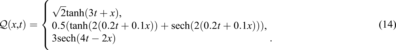
In this context, we used the Khater II scheme to the 3-FNLS27-31 to evaluate an unlimited number of solutions and then used the TQBS scheme32,33 to determine the absolute value of error between the precise and numerical solutions. The three-FNLS equation is denoted by ref. 34


This study paper’s remaining parts are organized as follows: The Khater II technique is used in the section Applications to find new solitary solutions to the 3-FNLS problem. Additionally, the TQBS numerical scheme is used to evaluate numerical solutions and determine the absolute error value between the computational and numerical solutions. The section Results and Discussion explains the findings and provides a physical description of the drawings that are shown. The section Conclusion summarizes the results of this investigation and the paper’s contributions.
Applications
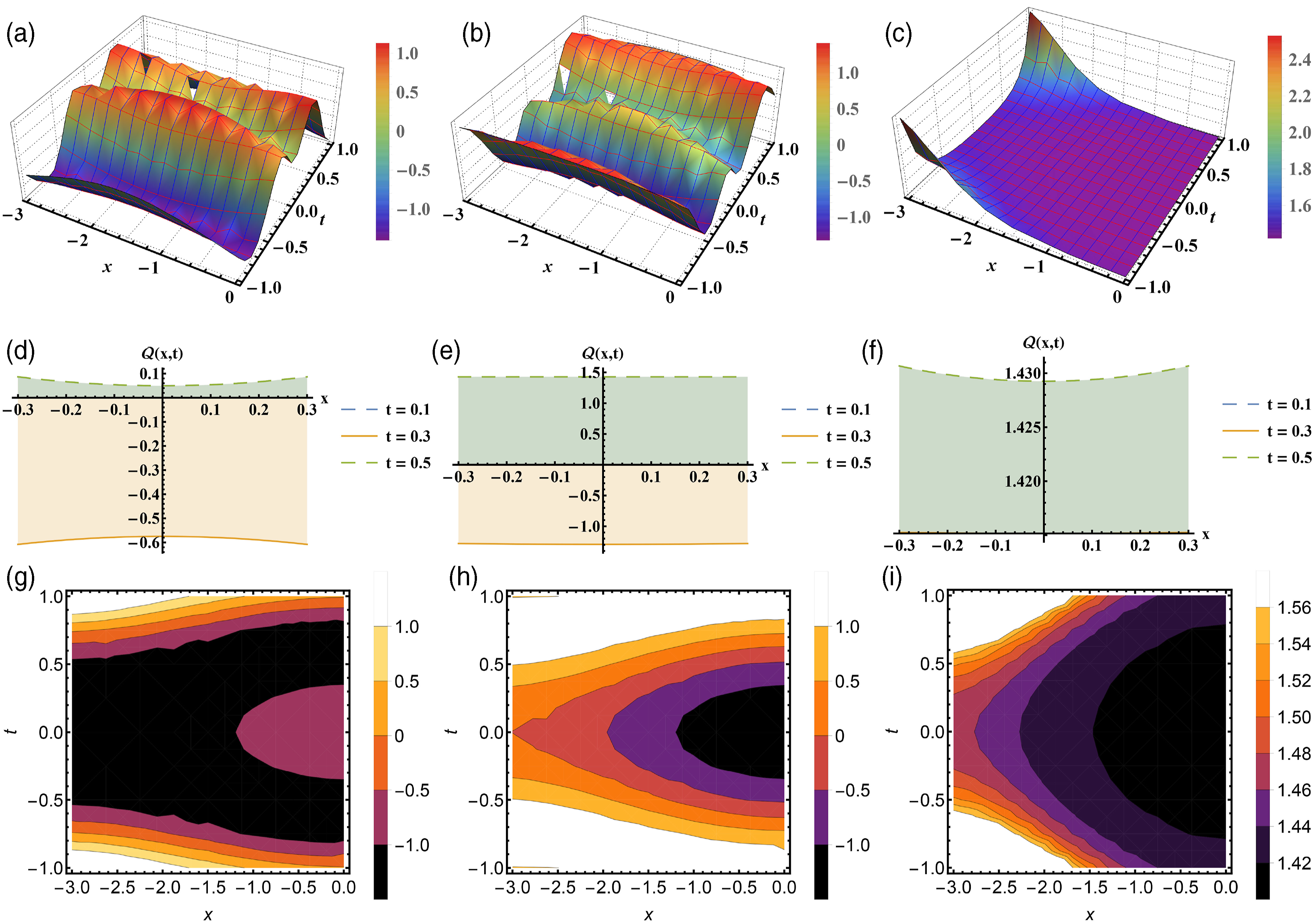
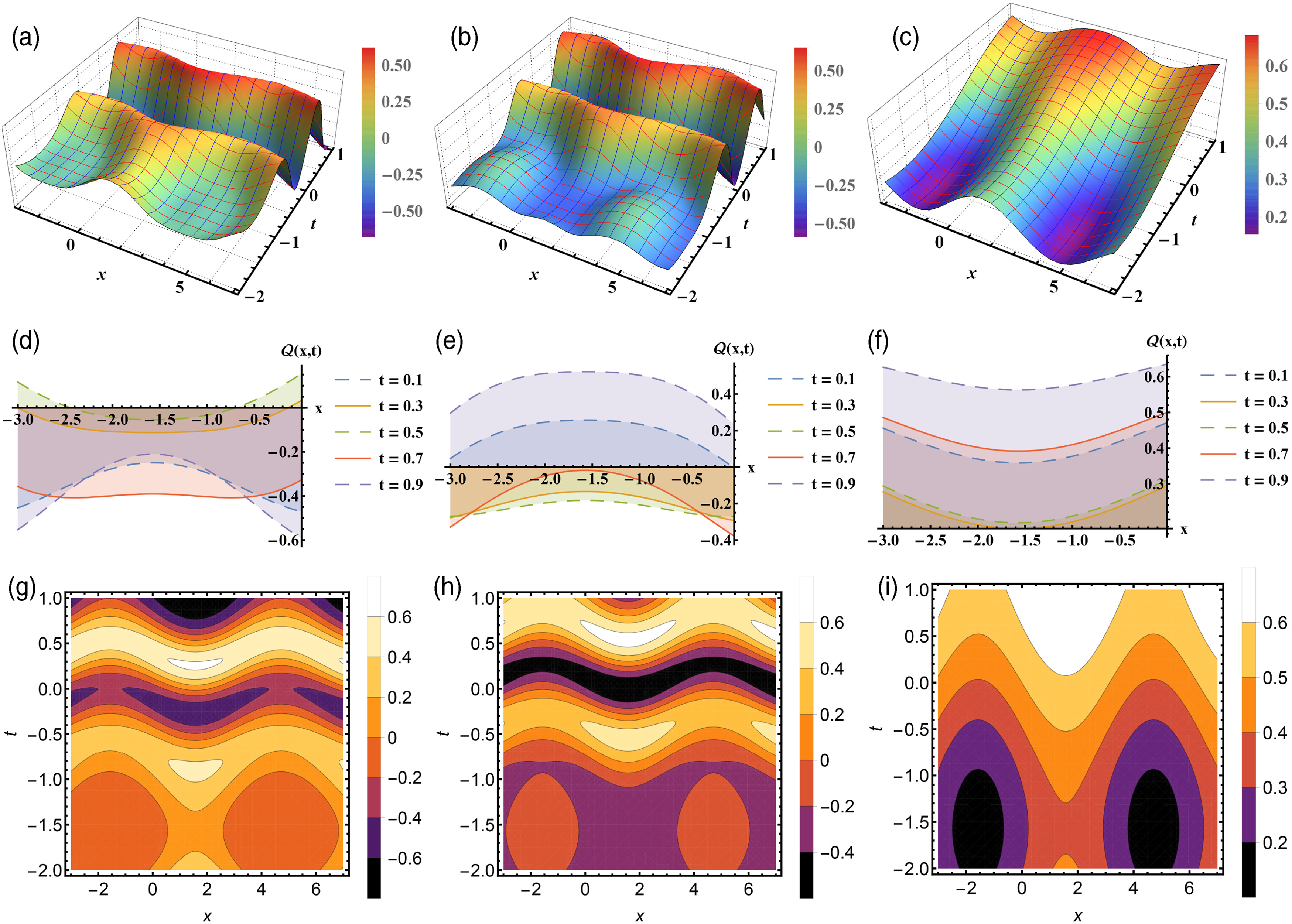
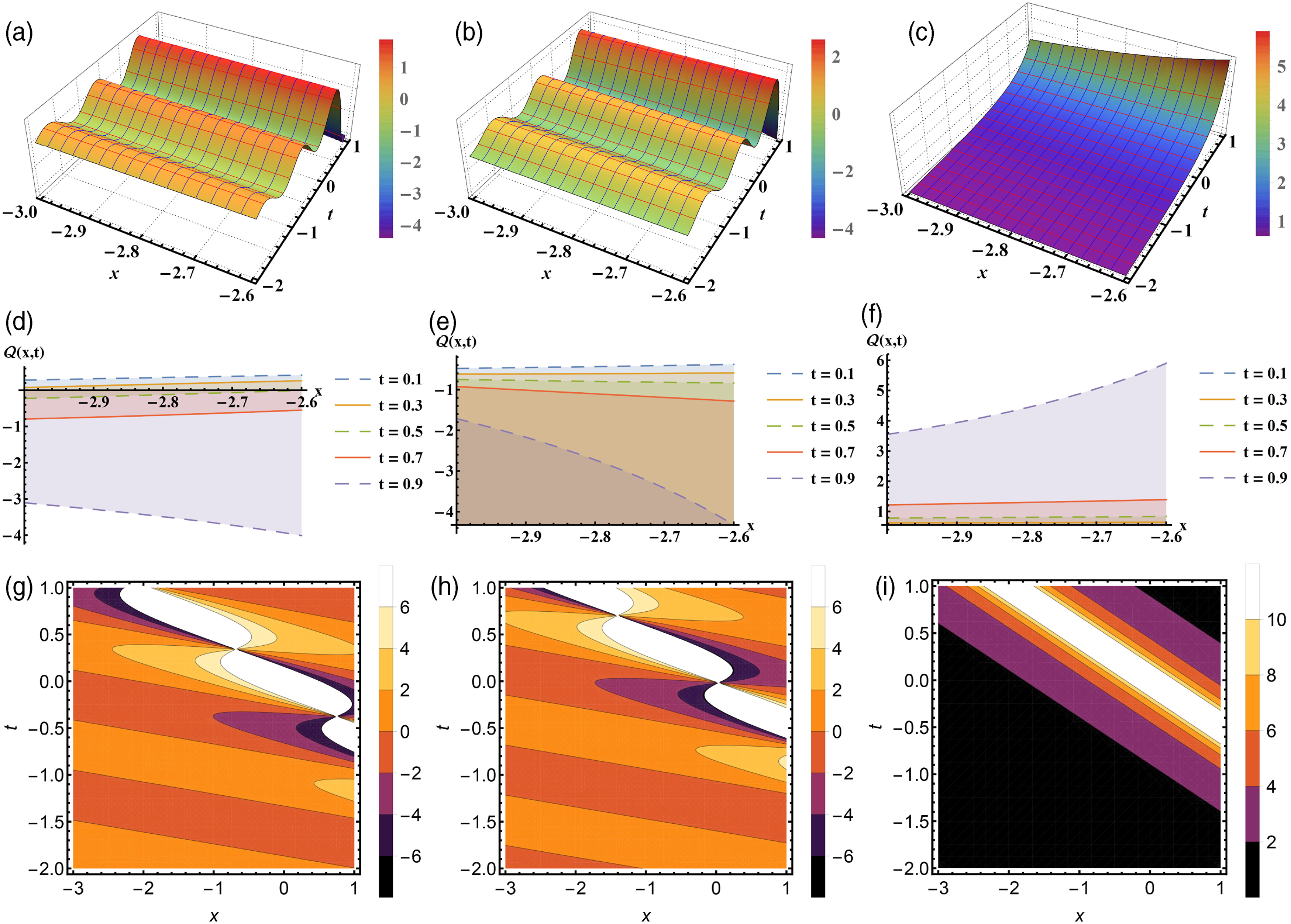
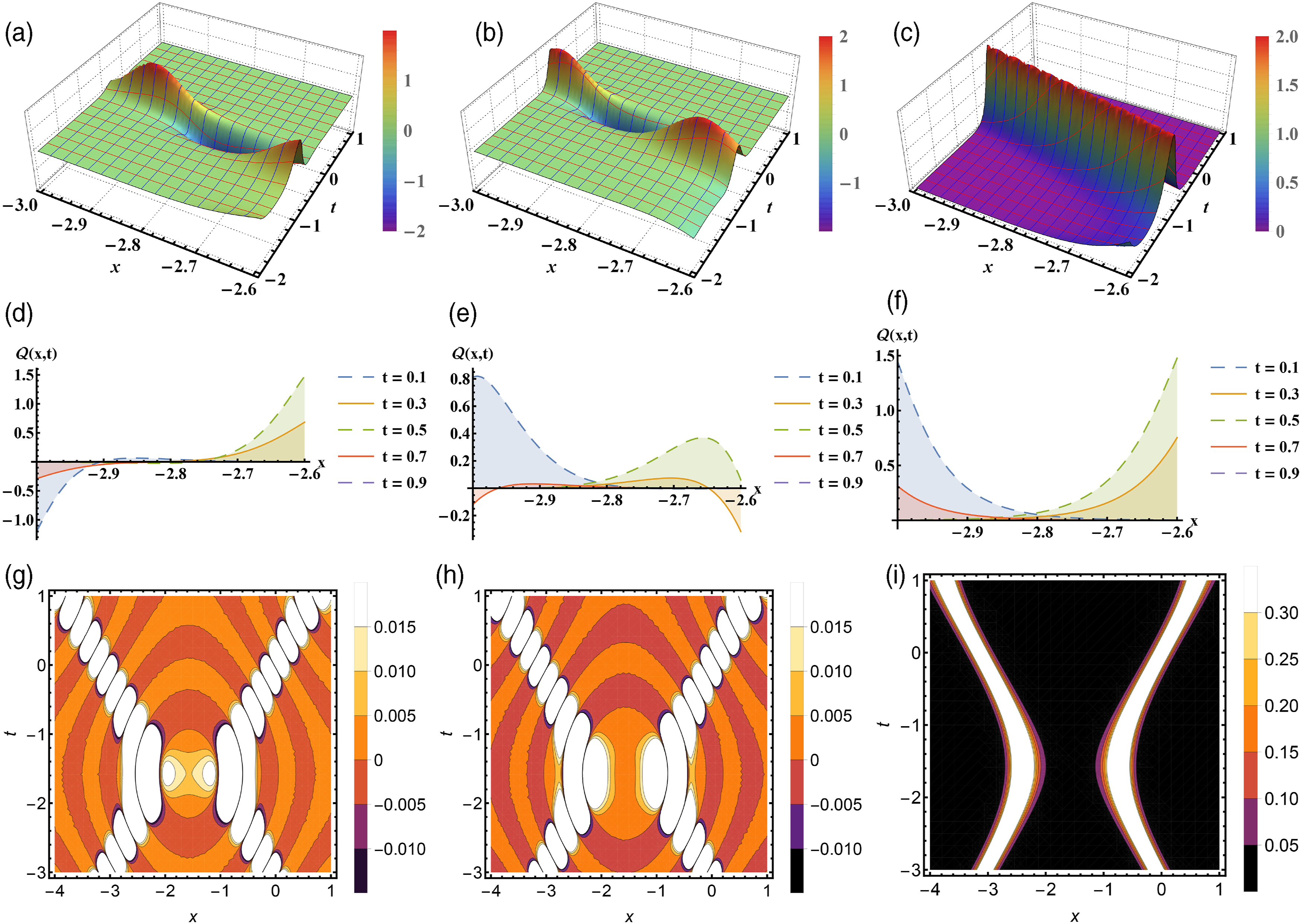
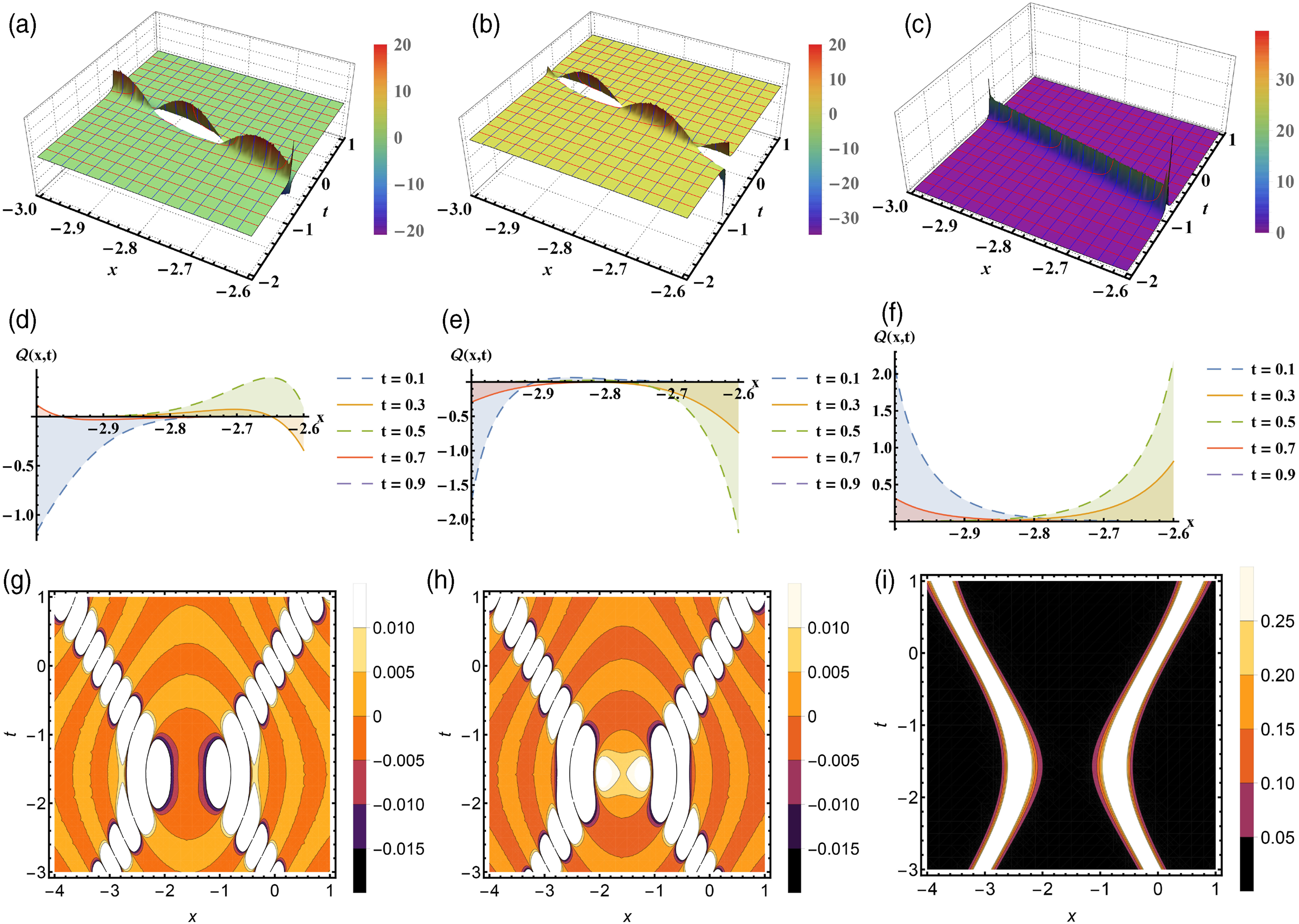
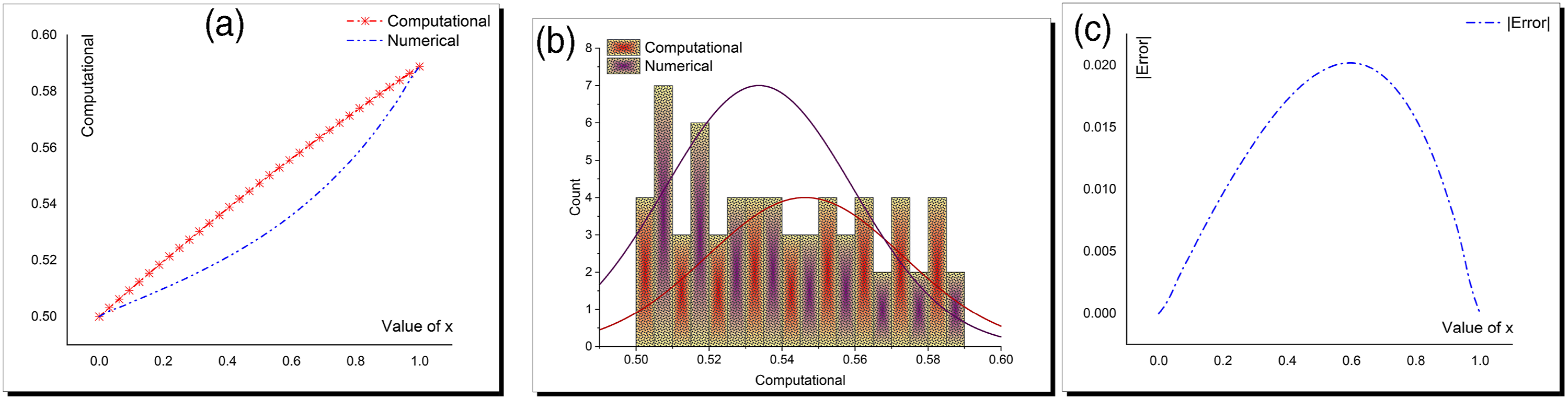
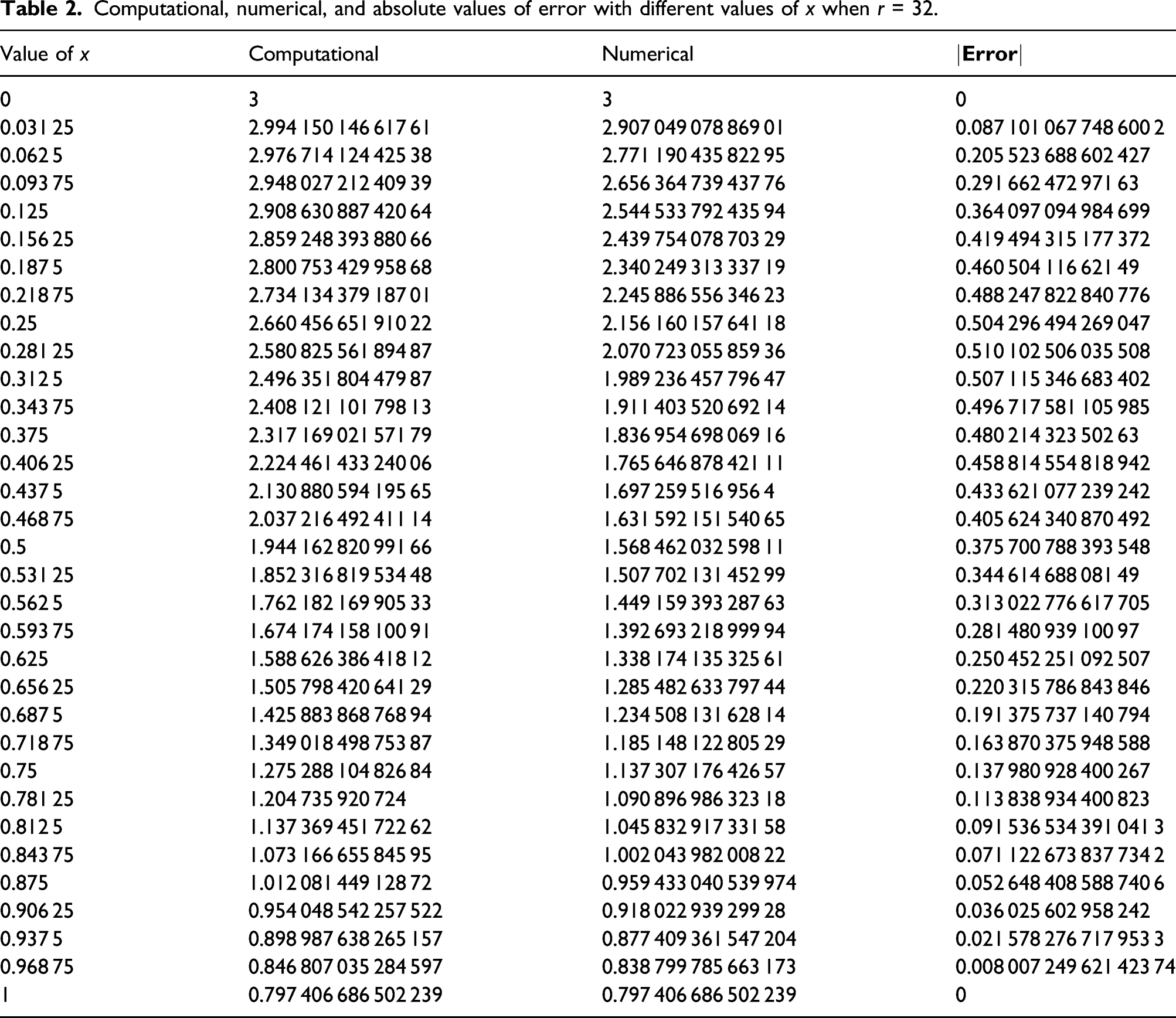
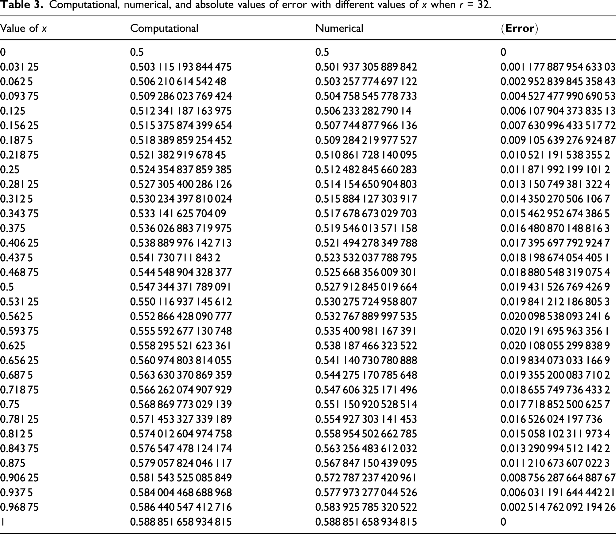
Here, the analytical and approximate solutions of the conformable fractional NLS equation are investigated by employing the suggested schemes. This study’s goal is to construct novel solutions’ structures and check their accuracy by calculating the absolute value of error between analytical and approximate solutions (Figures 1–10). Graphical representations of equation (8) for the real, imaginary, and absolute values of the Graphical representations of equation (9) for the real, imaginary, and absolute values of the Graphical representations of equation (10) for the real, imaginary, and absolute values of the Graphical representations of equation (11) for the real, imaginary, and absolute values of the Graphical representations of equation (12) for the real, imaginary, and absolute values of the Graphical representations of equation (13) for the real, imaginary, and absolute values of the Computational, numerical, and absolute value of error according to the shown Table 1. Computational, numerical, and absolute value of error according to the shown Table 2. Computational, numerical, and absolute value of error according to the shown Table 3.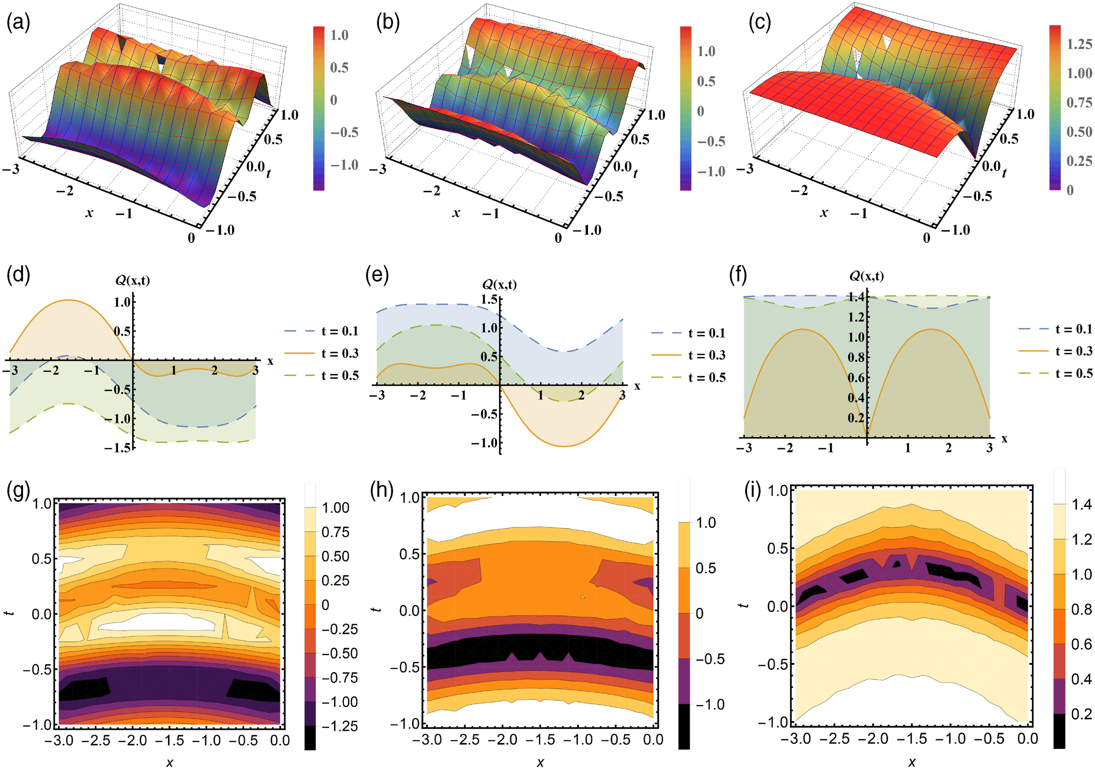
Solitons wave solutions
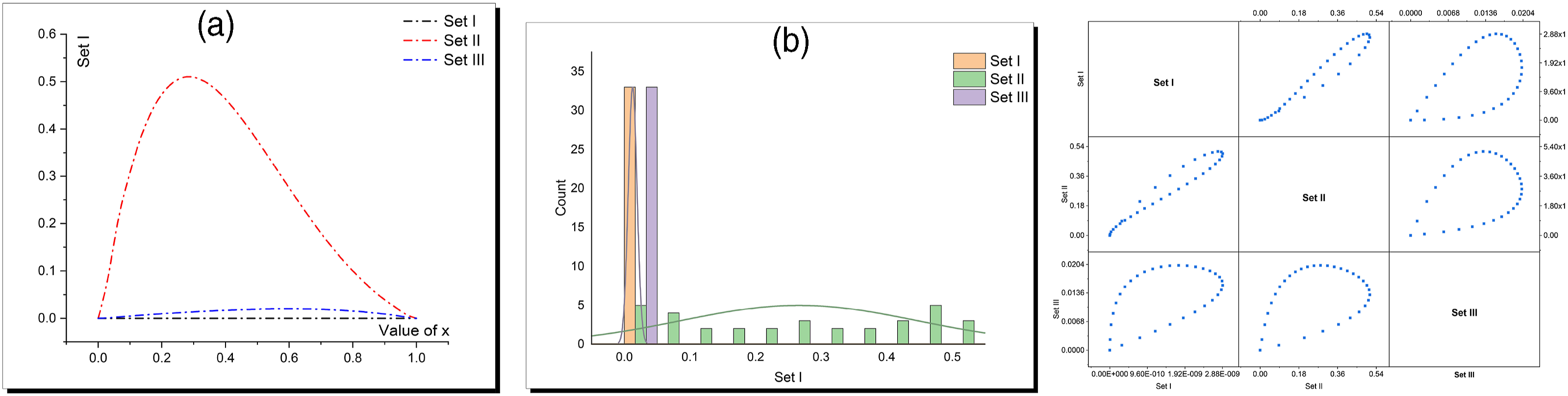
Applying the Khater II method to the considered model for investigating the soliton wave solutions, gets the following values of the above-shown parameters: Set I


For δ ≠ 0, we obtain


Approximate solutions
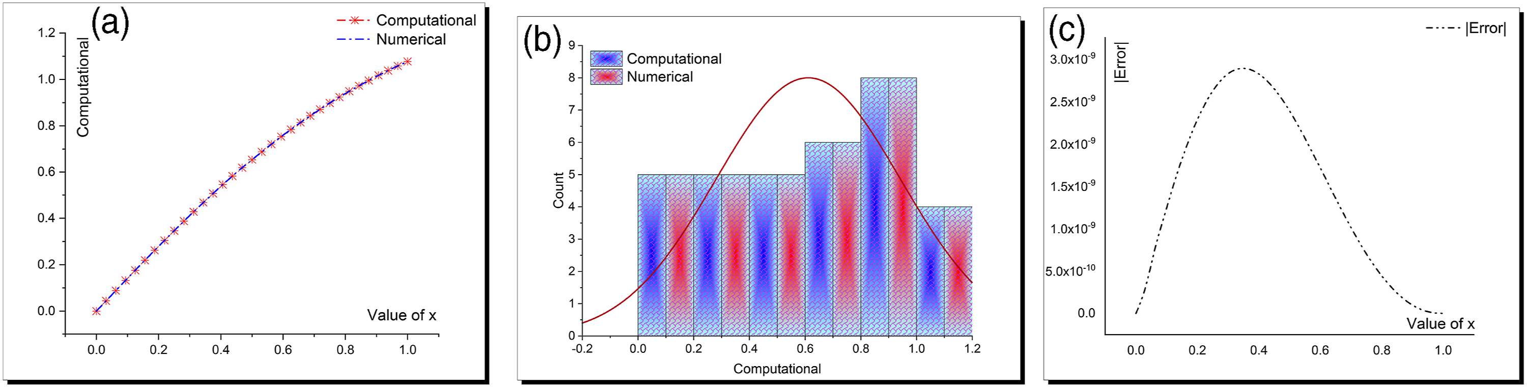
Computational, numerical, and absolute values of error with different values of x when r = 32.
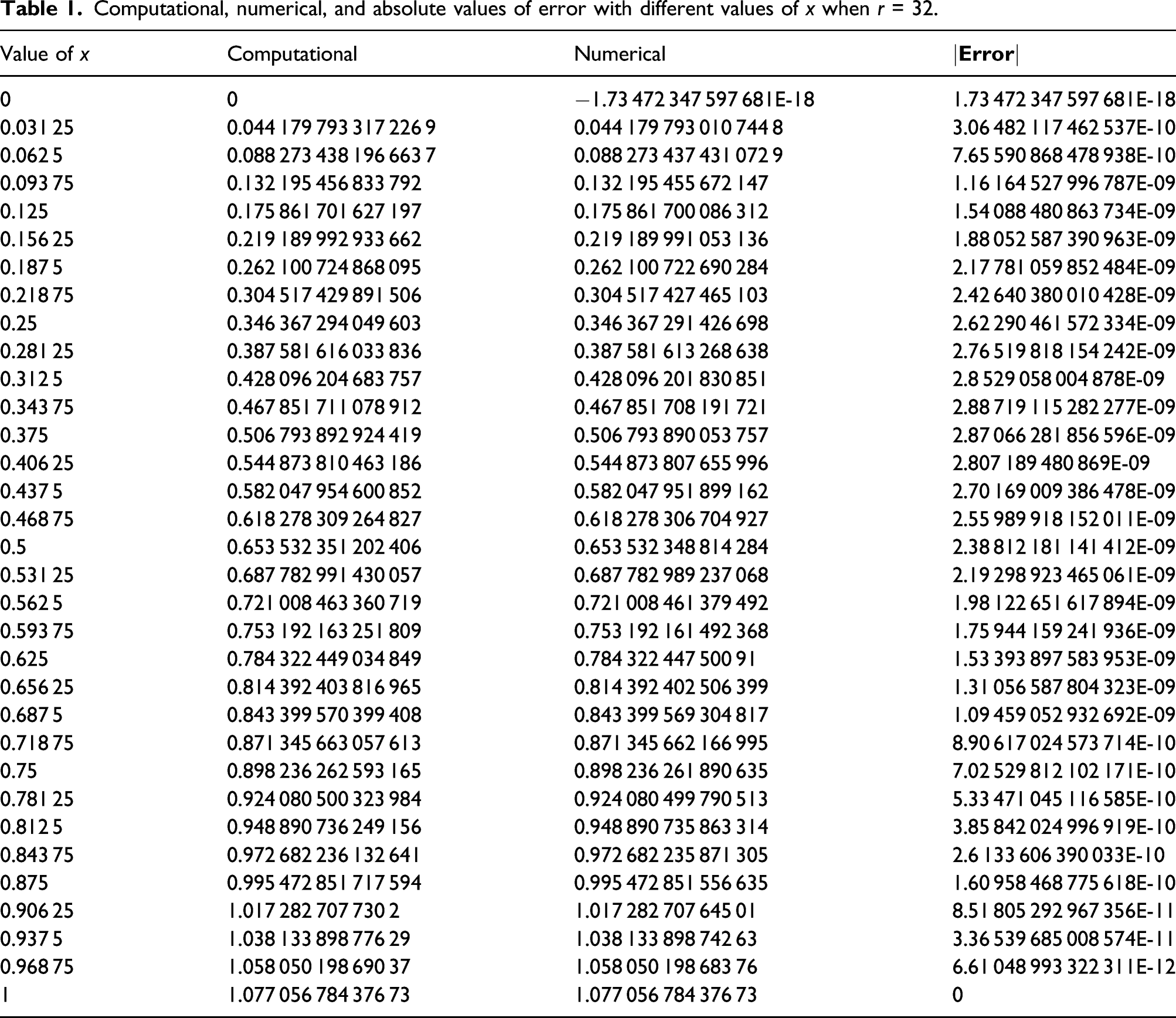
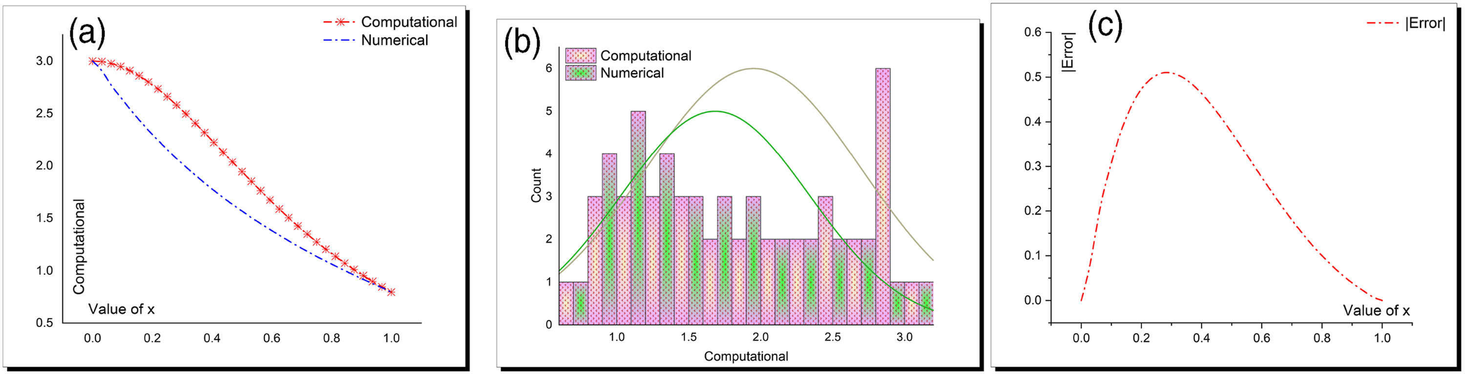
Computational, numerical, and absolute values of error with different values of x when r = 32.
Computational, numerical, and absolute values of error with different values of x when r = 32.
Results and discussion
This part explores the paper’s findings and innovation by exhibiting the benefits of the analytical and numerical techniques utilized, the acquired results, and their comparison to previously published solutions, ultimately proving the correctness of the found solutions. Finally, we will analyze the physical meaning of the numbers presented. Mostafa M. A. Khater discovered the Khater II technique for the first time. He created this extended technique in order to get innovative structures for explicit wave solutions to a class of nonlinear evolution equations. The efficacy and potency of this technique have been established. 35 The TQBS scheme has been employed to find the numerical solutions of the investigated model based on the obtained solutions (8), (10), (12). The analytical solutions have been explained through some different graphs (1, 2, 3, 4, 5, 6). While the matching between both solutions is explained through some distinct plots (7, 8, 9). Comparing our solutions to show the solutions’ accuracy leads to verify our obtained solutions and superiority of equation (8) over other constructed solutions.
Conclusion
The 3-FNLS model was effectively studied in this research work using the Khater II approach. Numerous separate precise solutions for moving and isolated waves have been discovered. These solutions have been illustrated using a variety of drawings that demonstrate additional and unexpected aspects of the fractional models under consideration. Our acquired answers have been discussed in terms of their correctness and uniqueness. Additionally, the potency and usefulness of the approaches utilized are discussed and validated.
Footnotes
Acknowledgment
We greatly thank Taif University for providing fund for this work through Taif University Researchers Supporting Project number (TURSP-2020/52), Taif University, Taif, Saudi Arabia.
Authors’ contribution
Dexu Zhao and Mostafa Khater have revised the conceptualization, data curation, and methodology. Dianchen Lu and Mostafa Khater have revised Data curation, Investigation, and Software. Samir Salama and Piyaphong Yongphe have revised the physical meaning of the obtained solutions and raised the given graphs resolutions. All authors have read and agreed to the published version of the manuscript.
Declaration of conflicting interests
The author(s) declared no potential conflicts of interest with respect to the research, authorship, and/or publication of this article.
Funding
The author(s) disclosed receipt of the following financial support for the research, authorship, and/or publication of this article: We greatly thank Taif University for providing fund for this work through Taif University Researchers Supporting Project number (TURSP-2020/52), Taif University, Taif, Saudi Arabia.
Availability of data and material
The data that support the findings of this study are available from the corresponding author upon reasonable request.
Code availability
The used code of this study is available from the corresponding author upon reasonable request.