Sage Journals: Discover world-class research

Abstract

An efficient method for solving vibration equations is the basis of the vibration analysis of a cracked multistage blade–disk–shaft system. However, dynamic equations are usually time varying and nonlinear, and the time required for solving is greatly increased accompanied by an increase in the model order caused by the multistage system and the nonlinearity caused by cracks. In this article, an efficient method for solving the time varying and nonlinear vibration equation is investigated. In the proposed method, the time varying terms are transformed into constant terms, while the local nonlinear matrix of the cracked blade is separated from the assembly stiffness matrix under the constraint of proper orthogonal decomposition (POD) transformation rules. Furthermore, the POD transformations of the constant terms and the linear assembled stiffness matrix can be implemented in the pretreatment steps to achieve a more efficient POD reduction operation. This research provides a method for efficiently performing the comprehensive and rapid analysis of nonlinear vibration characteristics of rotor systems.

Keywords

Efficient solution method time varying coefficient nonlinearity vibration equation multistage blade–disk–shaft system

Introduction

Blades generally play a significant role in turbomachinery, and damage monitoring of rotating blades is becoming a popular research topic. Vibration modeling and characteristic analysis are the basis of damage monitoring. The model of a blade–disk–shaft system mainly includes the lumped-parameter model, the finite element model, and the continuous parameter model.^1–5 Compared with the performance of the lumped-parameter model and the finite element model, the continuum model has higher precision, clearer analytical expression and higher computational efficiency, and has been widely used.

However, with the increase in the model order caused by a multistage system and the nonlinearity caused by cracks, the time required to solve the vibration equation is greatly increased, which affects the efficiency of vibration analysis. Therefore, the ability to rapidly solve nonlinear equations is particularly important. There are two approaches to quickly solve such equations, that is, constructing and optimizing the solution method and dimension reduction of the model.

In the research on solution methods for nonlinear equations, a large number of analytical, approximate analytical, and numerical methods have been proposed. Anjum and He⁶ combined the variational iteration method with the techniques of the Laplace transform to find the approximate nonlinear frequency and approximate analytic solution of the model problem in microelectromechanical systems. Akuro and Chinwuba⁷ used the continuous piecewise linearization method to solve the equations of coupled nonlinear models of a fixed-end two-mass system. Moreover, they investigated the effect of the mass ratio on the response. He et al.⁸ proposed an approach to obtain the approximate periodic solutions of nonlinear oscillators. Then, they derived the frequency–amplitude relationship by adopting He’s frequency formulation. Noeiaghdam et al.⁹ specifically designed the homotopy perturbation method to solve a second kind of linear Volterra integral equation and found the optimal approximation and optimal error. He and El‐Dib¹⁰ discussed the solution and the stability conditions of the third-order Duffing equation by using the reducing rank method with the homotopy perturbation method. Biswal et al.¹¹ used the homotopy perturbation method to obtain the velocity profile of fluid flow for the Jeffery–Hamel problem. Lu and Zheng¹² explored the full power of the Adomian decomposition method (ADM), and they demonstrated the standard ADM and ADM with an integration factor to calculate explicit closed-form solutions of first-order scalar partial differential equations. Lichae et al.¹³ adopted the asymptotic Adomian decomposition method (AADM) to solve the fractional order Riccati differential equations. Bavi et al.¹⁴ solved the nonlinear vibrations of rotor–stator contact in a two-degree-of freedom model by employing Runge–Kutta numerical methods. They also analyzed the effect of gravity, damping, and asymmetry on the rotor response. Zhan¹⁵ analyzed the order conditions of high-order explicit exponential Runge–Kutta methods for stiff semilinear delay differential equations. Vermeire and Hedayati Nasab¹⁶ introduced a family of accelerated implicit explicit Runge–Kutta schemes for solving stiff system equations. Akbas¹⁷ used the Newmark average acceleration method to solve the free vibration responses and the forced vibration responses of the axially functionally graded beam. Liu et al.¹⁸ solved the free vibration and transient dynamic behaviors of functionally graded material on the basis of Newmark’s method.

The above methods provide efficient ways to solve nonlinear equations. Analytical and approximate analytical methods can be employed to analyze the influence of various parameters on the solution, which can provide intuitive graphical analysis of the solution. However, the solution and derivation of such methods are cumbersome; thus, this approach is difficult to apply to large-scale equations that lack simple analytical expressions. In the numerical method, the solutions are composed of numerical points. The disadvantage is that the development trend of the solution and the influence of related parameters cannot be directly analyzed, but a large number of complicated formula derivation steps can be reduced, which has advantages in solving large-scale and nonlinear vibration equations without simple analytical expressions.

With the intention of analyzing large-scale nonlinear vibration equations of a cracked bladed disk rotor system, scholars have also performed extensive research on the dimension reduction of the vibration model to quickly solve transient and steady-state vibration responses. Wang et al.¹⁹ employed the complex free interface component mode synthesis method to reduce the order of a model. Pourkiaee and Zucca²⁰ employed the Craig–Bampton method and modal synthesis based on loaded interface modeshapes to present a new reduced-order model for the nonlinear vibration analysis of mistuned bladed disks with shrouds. Joannin et al.²¹ introduced a novel reduced-order modeling technique combining the concepts of nonlinear complex modes with characteristic constraint modes. Sun et al.²² proposed a novel framework in which the sophisticated geometrical structure was considered by the finite solid element method, and efficient model order reduction was applied to the model. Alsaleh et al.²³ demonstrated that a two-degree-of-freedom (DOF) model could predict flexural vibrations under rigid conditions with an error of less than 5%. They also illustrated the applicability of employing simple models to predict the dynamic response of a real rotor system. The above studies provide important methods and strategies for dimension reduction of vibration equations, and each method has its own advantages and application scope.

Another kind of dimension reduction method is proper orthogonal decomposition (POD), and its advantage is that it can reduce a system with moderate order to that of a very small order. Therefore, POD has been widely applied in the field of nonlinear research. Vergari et al.²⁴ developed a reduced-order model for heat transfer problems in computational fluid dynamics that relied on the POD. Yu et al.²⁵ reduced a 22-DOF nonlinear system of a high-pressure rotor to a 2-DOF system, preserving the oil film oscillation property by employing a modified POD method. Im et al.²⁶ proposed a new reduction process in which the dynamic substructures were reduced via POD. Lu et al.²⁷ proposed a modified nonlinear POD method to reduce the order of the multiple DOFs of a rotor system. Sidhu et al.²⁸ introduced a sparse proper orthogonal decomposition–Galerkin methodology for the model dimension reduction of nonlinear parabolic partial differential equation systems. Nguyen et al.²⁹ employed the POD technique to project the original large-scale full chemical process model onto a small system with a reduced model space. Jin et al.³⁰ proposed a new adaptive POD method to address the weakness of the local property of the interpolation tangent-space of the Grassmann manifold method. Eftekhar Azam et al.³¹ provided effective online estimations of the possible structural damage by tracking the time evolution of stiffness parameters in the model order reduction procedure. Luo³² presented a hybrid model method based on POD for the aerodynamic design optimization of a low-speed 4.5-stage compressor.

Compared with the order of the finite element model, the order of the continuum model of the blade–disk–shaft system discretized by the assumed modal method is very low; thus, it is more suitable to adopt the POD reduction method. However, if the POD method is directly applied to time varying and nonlinear equations, the POD transformation must be performed in each iteration process but not in the pretreatment step. Therefore, although the POD reduces the order of the equation, the POD transformation in the iterative process increases the calculation time, which results in the failure to reduce the time consumption.

Based on the analysis of the literature and the summary of the problems described above, a continuum dynamic model of a cracked multistage blade–disk–shaft system is established in Dynamic model of a multistage blade–disk–shaft system to illustrate the inevitability of introducing nonlinearities and time varying coefficients into the model. Furthermore, based on the POD method, an efficient method referred to as constant coefficients local nonlinearity POD (CC_LNLPOD) is proposed in Proposed CC_LNLPOD method to solve time varying and nonlinear equations. Then, in Comparison of the results of different solving methods, the accuracy and time consumption of the proposed method are compared with those of other methods. Finally, the conclusions are drawn in Conclusions.

Dynamic model of a multistage blade–disk–shaft system

In this section, a continuum dynamic model of a cracked multistage blade–disk–shaft system is established to illustrate the inevitability of introducing nonlinearity and time varying coefficients into vibration equations. After that, the shortcomings of conventional numerical methods in solving time varying and nonlinear equations of multistage bladed disk rotor systems are further discussed.

Modeling of a normal system

First, the absolute coordinates of the microunit of continuum components (shafts, disks, and blades) are established in a fixed coordinate system. The velocity expression is then obtained by derivation of the time variant coordinates (displacements). On this basis, the kinetic and potential energy equations of the components are obtained by integration. Then, the energy equations are discretized by the assumed modal method, while the vibration equations about generalized coordinates are established based on the Lagrange equation.

The schematic diagram of the multistage blade–disk–shaft system is shown in Figure 1, and it contains a bending and torsional shaft, three disks, and flexible blades fixed onto the outer edge of the disk with a setting angle β. oxyz denotes the global coordinate, Px_iy_iz_i is the rotating coordinate attached to the i^th disk with a rotational speed Ω, and z_di is the coordinate of the i^th disk in the z-axis. h_d and h_b represent the thicknesses of the disk and blade, respectively.

Figure 1.

Schematic diagram of the multistage bladed disk rotor system.

Based on the hypothesis of small deformation, the motion of the blade–disk–shaft system can be projected in three planes (oxy, ozx, and ozy) along three coordinate axes. One of the disks is taken as an example, and the motion decomposition is shown in Figures 2 and 3. The omitted view in the ozy plane is similar to that of Figure 2. The bold line represents the rigid body displacement of the component, while the dashed line represents the elastic deformation of the component.

Figure 2.

Decomposition of motion in the ozx plane.

Figure 3.

Decomposition of motion in the oxy plane.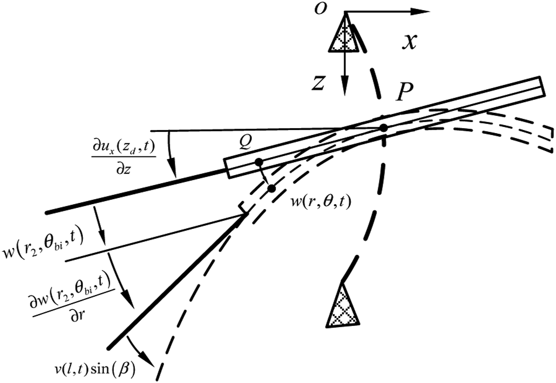

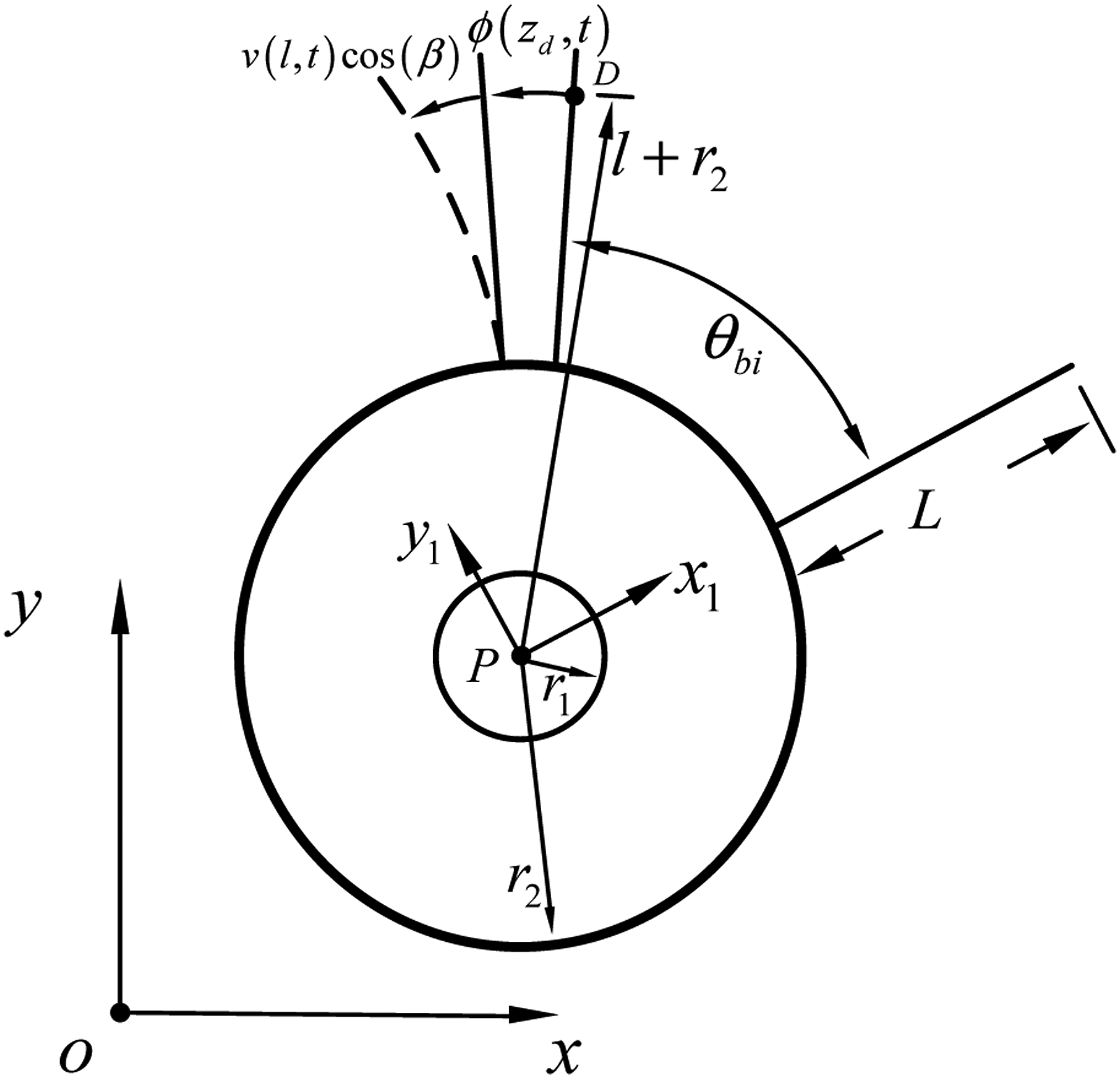
Figure 2 shows a schematic diagram of the decomposition of motion in the ozx plane. In this figure, Q is an arbitrary microunit in the disk, $w (r, θ, t)$ denotes the deflection of the disk at arbitrary position $(r, θ)$ , and $(r, θ)$ is the local polar coordinate system in the disk. $u_{x} (z, t)$ denotes the deflection of the shaft in the x-direction. $\partial u_{x} (z_{d}, t) / \partial z$ is the rotation of the cross section of the shaft at z_d. $w (r_{2}, θ_{b i}, t)$ is the deflection of the disk at $(r_{2}, θ_{b i})$ , where r₂ represents the external diameter of the disk and $θ_{b i}$ represents the reference angle of the i^th blade. $\partial w (r_{2}, θ_{b i}, t) / \partial r$ is the dip angle of the disk where the i^th blade is set. $v (l, t) \sin (β)$ denotes the out-of-plane deflection of the blades.

Figure 3 shows a schematic diagram of the decomposition of motion in the oxy plane. In this figure, D is an arbitrary microunit in the blade, its distance from the root of the blade is l, and L is the length of the blade. The direction of the x_i-axis is coincident with the spanwise direction of the reference blade (the first blade). r₁ and r₂ are the inner diameter and outer diameter of the disk, respectively. $ϕ (z_{d}, t)$ denotes the torsional displacement of the shaft. $v (l, t) \cos (β)$ denotes the in-plane deflection of the blades.

According to the decomposition of motion and coordinate system settings described above, the coordinates of arbitrary microunits in the shaft during the rotation of the rotor and the structural elastic vibration with respect to the fixed coordinate system can be expressed as follows

u = (u_{x} (z), u_{y} (z), z)

(1)In the same way, the coordinates of arbitrary microunit Q in the disk with respect to the fixed coordinate system can be expressed as

(x_{Q}, y_{Q}, z_{Q})

, and the coordinates of arbitrary microunit D in the blade with respect to the fixed coordinate system can be expressed as

(x_{D}, y_{D}, z_{D})

The velocity expression can be obtained through the derivation operation of the time variant coordinates (displacements). Based on the consideration of the translational motion and the rotation around the z-axis, the total kinetic energy of the shaft can be acquired by integrating the kinetic energy of the microunit along the shaft

T_{s} = \frac{1}{2} ρ_{s} A_{s} \int_{0}^{s} ({\dot{u}}_{x}^{2} + {\dot{u}}_{y}^{2}) d z + \frac{1}{2} ρ_{s} I_{s p} \int_{0}^{s} {(Ω + \dot{ϕ})}^{2} d z

(2)where S is the length of the shaft, ρ_s denotes the density, A_s is the area of the cross section of the shaft, and I_sp is the polar moment of inertia.

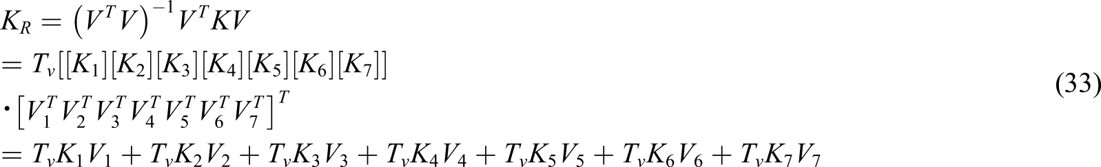
According to elasticity theory, the torsion and bending of the shaft are considered, and the total potential energy of the shaft can be given as follows³³

U_{s} = \frac{1}{2} E_{s} I_{s x} \int_{0}^{s} ({(\frac{\partial^{2} u_{x}}{\partial z^{2}})}^{2} + {(\frac{\partial^{2} u_{y}}{\partial z^{2}})}^{2}) d z + \frac{1}{2} G_{s} I_{s p} \int_{0}^{s} {(\frac{\partial φ}{\partial z})}^{2} d z

(3)where E_s and G_s are the Young’s modulus and shear modulus, respectively. I_sx is the area moment of inertia on the x₁-axis.

In this study, the disk is assumed to be a rigid body without considering its elastic deformation. Moreover, the inertia product and moment of inertia of the disks are relatively large, so the disk cannot be treated as particles. Therefore, the translational and rotational kinetic energy of the j^th disk is as follows

T_{d j} = \frac{1}{2} ρ_{d} h_{d} \int_{r_{1}}^{r_{2}} \int_{0}^{2 π} ({\dot{x}}_{Q}^{2} + {\dot{y}}_{Q}^{2} + {\dot{z}}_{Q}^{2}) r d r d θ

(4)In the same way, the kinetic energy associated with the i^th blade can be obtained as follows

T_{b i} = \frac{1}{2} ρ_{b} A_{b} \int_{0}^{L} ({\dot{x}}_{D}^{2} + {\dot{y}}_{D}^{2} + {\dot{z}}_{D}^{2}) d l

(5)The kinetic energy for all the blades in the j^th disk is as follows

T_{B j} = \sum_{i = 0}^{N_{j} - 1} T_{b i}

(6)where N_j is the number of blade in the j^th disk.

The bending potential energy and centrifugal potential energy of the i^th blade can be given as follows³⁴

U_{b i} = \sum \frac{1}{2} M d θ = \frac{1}{2} E I \int_{0}^{L} {(\frac{\partial^{2} v_{i} (l, t)}{\partial r^{2}})}^{2} d l

(7)

U_{c i} = \frac{1}{4} ρ A_{b} Ω^{2} \int_{0}^{L} [{(r_{2} + L)}^{2} - {(r_{2} + l)}^{2}] {(\frac{\partial v_{i} (l, t)}{\partial l})}^{2} d l

(8)The equivalent coupling potential energy between blades can be calculated as follows

U_{couple} = \sum_{i = 0}^{N - 1} \frac{1}{2} \int_{0}^{L} k_{i} (l) {(v_{i + 1} (l, t) - v_{i} (l, t))}^{2} d l

(9)where

k_{i} (l)

denotes the equivalent coupling stiffness between the blades.

Then, the total potential energy of the blades in the j^th disk can be given as follows

U_{B j} = \sum_{i = 0}^{N_{j} - 1} (U_{b i} + U_{c i}) + U_{couple}

(10)The assumed mode method is adopted to discretize the continuous system. The displacements of the shaft can be expressed as follows³³

u_{x} (z, t) = U^{T} q_{x} = q_{x}^{T} U

(11)

u_{y} (z, t) = U^{T} q_{y} = q_{y}^{T} U

(12)

ϕ (z, t) = Φ^{T} q_{ϕ} = q_{ϕ}^{T} Φ

(13)where

U

and

Φ

denote the assumed modal matrix

q_{x}

and

q_{y}

, and

q_{ϕ}

denotes the generalized coordinate associated with the shaft.

In a similar way, the displacements of the blade can be expressed as follows³⁴

v (l, t) = V^{T} q_{v} = q_{v}^{T} V

(14)where

V

denotes the assumed modal matrix associated with the blade and

q_{v}

denotes the generalized coordinate of the blade.

The equations above are substituted into the energy expressions, and the Lagrange equations are employed to yield the following discretized equations of motion in matrix notation

\frac{d}{d t} (\frac{\partial L}{\partial \dot{η}}) - \frac{\partial L}{\partial η} = Q

(15)

L = T - U = T_{s} - U_{s} + \sum_{j = 1}^{n} T_{d j} + T_{B j} - U_{B j}

(16)where

η

denotes the generalized coordinate matrix,

Q

is the generalized force matrix corresponding to the generalized coordinates, and the bending torsion coupling excitation caused by the eccentricity of the disk is also considered. The discretized equations of motion in matrix notation can be given as follows

M \ddot{η} + C \dot{η} + Kη = Q

(17)The detailed expressions associated with the generalized coordinates

q_{x}

q_{y}

q_{ϕ}

, and

q_{v}

are shown in equations (37)–(40), respectively, in Appendix 1.

Multistage blade–disk–shaft system with a cracked blade

In the modeling of a cracked blade, the released energy associated with the crack is considered as follows^33,35

U_{c} = \frac{1}{2} \frac{{(E I)}^{2}}{K_{crack}} η^{T} V (l_{c}) ″ V {(l_{c})}^{″ T} η

(18)where

K_{crack}

is the breathing stiffness of the crack, which can accurately consider the influence of the centrifugal effect and bending vibration on the crack. The breathing function can be found in our recent publication³⁵

K_{crack} = k_{c} \times {\begin{matrix} \infty \\ {(\frac{h / 2 - y_{c}}{y_{0} - y_{c}})}^{3} \\ 1 \end{matrix} \begin{matrix} σ_{b} \geq \frac{σ_{d}}{y_{c}} \\ \frac{σ_{d}}{((h / 4) + (y_{c} / 2))} < σ_{b} < \frac{σ_{d}}{y_{c}} \\ σ_{b} \leq \frac{σ_{d}}{((h / 4) + (y_{c} / 2))} \end{matrix}

(19)where

σ_{b}

is the bending stress,

σ_{d}

is the centrifugal stress, and

k_{c}

is the stiffness of the open crack,³⁶ which can be expressed as follows

k_{c} = \frac{E I}{6 (1 - μ^{2}) h Q (γ)}

(20)The kinetic energy, bending potential energy, and centrifugal potential energy are the same as those of a normal blade. In the same way, the assumed mode method and Lagrange equation are used to construct the coupling vibration equation associated with the cracked blade

\begin{matrix} \begin{array}{l} M_{v} {\ddot{q}}_{v} + C_{v} {\dot{q}}_{v} \\ + (K_{v} - \cos^{2} (β) Ω^{2} M_{v} + \frac{1}{2} (K_{Ω} + K_{Ω}^{T}) + 2 K_{cp} - \underline{\underline{K_{c}}}) q_{v} \\ - K_{cp} q_{v (i + 1)} - K_{cp} q_{v (i - 1)} \\ (- \cos (Ω t + θ_{b i}) M_{s v d z d s}^{T} - \sin (Ω t + θ_{b i}) M_{s d v z d s}^{T}) {\ddot{q}}_{x} \\ + (2 Ω \sin (Ω t + θ_{b i}) M_{s v d z d s}^{T}) {\dot{q}}_{x} \\ + (Ω^{2} \cos (Ω t + θ_{b i}) M_{s v d z d s}^{T}) {\ddot{q}}_{x} \\ (- \sin (Ω t + θ_{b i}) M_{s v d z d s}^{T} + \cos (Ω t + θ_{b i}) M_{s v d z d s}^{T}) {\ddot{q}}_{y} \\ (- 2 Ω \cos (Ω t + θ_{b i}) M_{s v d z d s}^{T}) {\dot{q}}_{y} \\ + (Ω^{2} \sin (Ω t + θ_{b i}) M_{s v d z d s}^{T}) q_{y} \\ + M_{ϕ v d z d ϕ}^{T} {\ddot{q}}_{ϕ} - Ω^{2} M_{ϕ v d z d ϕ}^{T} q_{ϕ} \end{array} & = Q_{v c} \end{matrix}

(21)where

K_{c}

is the additional stiffness caused by the crack, and it is calculated as follows³⁵

K_{c} = \frac{{(E I)}^{2}}{K_{crack}} V (l_{c}) ″ V {(l_{c})}^{″ T}

(22)Due to the accurate consideration of the centrifugal effect and bending vibration on cracks, nonlinearity is inevitably introduced into the vibration equations of blade–disk–shaft systems. Combining the equations associated with the shaft (equations (37)–(39)) that associated with the normal blade (equation (40)) and that of the cracked blade (equation (21)), the assembled vibration equation of the cracked multistage blade–disk–shaft system can be constructed as follows

M \ddot{η} + C \ddot{η} + K_{crack} η = Q

(23)

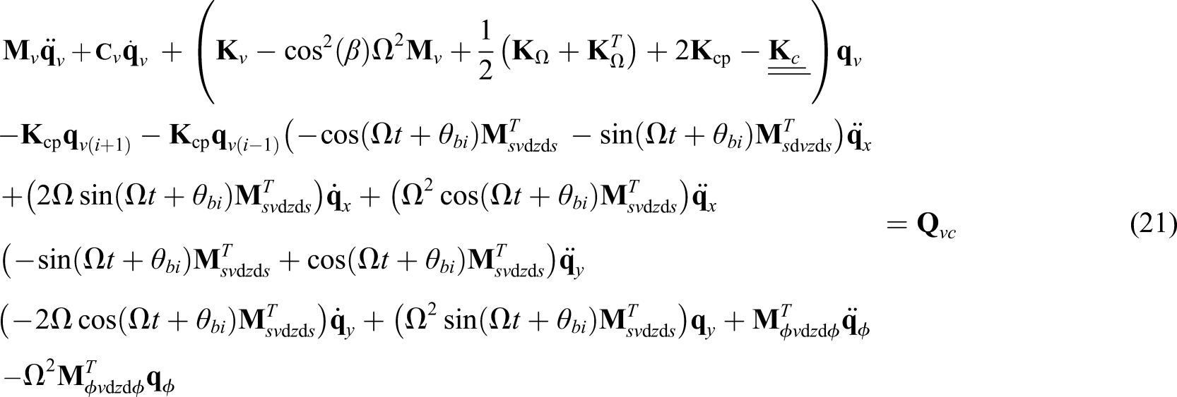
As seen in equations (21) and (37)–(40), the assembled vibration equation (equation (23)) is time varying and nonlinear.

Conventional solution for time varying and nonlinear equations

The Newmark-β direct integration method³⁷ is commonly used to solve the assembled vibration equation of the cracked blade–disk–shaft system with time varying coefficients and nonlinearities. The solving methodology is shown in Figure 4.

Figure 4.

Flowchart of the conventional solving method.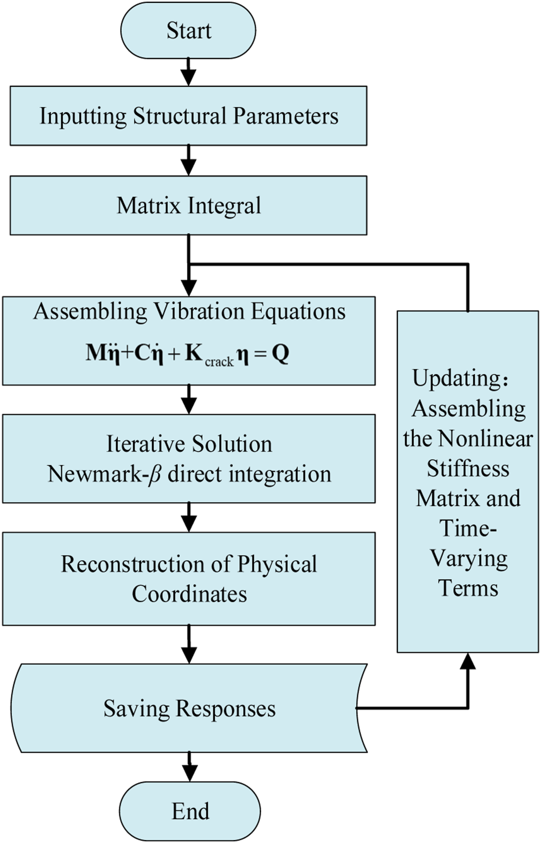

As seen in equations (37)–(40), there are many constant matrices with time varying coefficients in the assembled vibration equation, equation (23), and these constant matrices are obtained by the matrix integral of the assumed modal matrices, as shown in the “matrix integral” step.

Then, according to equations (21) and (37)–(40), the standard form of equation (23) can be assembled in the “assembling vibration equation” step.

After that, the Newmark-β direct integration method is adopted to solve the responses of the generalized coordinates at each iterative step in the “iterative solution” step.

Afterward, the responses of the physical coordinates are obtained by combining the responses of the generalized coordinates with the associated assumed modalities in the “reconstruction of physical coordinates” step.

At this time, the breathing state and instantaneous stiffness of the crack can be determined and calculated according to equation (19).

Finally, the assembled stiffness matrix and time varying terms are updated in the next time step.

With the increase in the model order caused by the multistage system and the nonlinearity caused by cracks, the time required to solve the vibration equation is greatly increased. Therefore, the above solving methodology needs to be optimized.

Proposed CC_LNLPOD method

Due to the influence of time varying coefficients and nonlinearity, POD dimension reduction needs to be carried out in the iterative process. Although the dimension can ultimately be reduced, the calculation time cannot be reduced. Therefore, on the basis of the POD method, an efficient solution method is proposed to optimize the solving methodology for time varying and nonlinear equations.

In the proposed method, two key transformations are adopted for the time varying and nonlinear equations so that the POD dimension reduction transformation of the large matrix can be carried out in the pretreatment step, which greatly reduces the calculation amount of the POD dimension reduction transformation in the iterative process and achieves a more efficient POD reduction operation.

First, the time varying coefficients of matrices are transformed into constant coefficients (CC) by introducing coordinate transformation and constructing equation transformation approaches. Then, matrix segmentation and separation strategies are proposed to separate the local nonlinear stiffness matrix of the cracked blade from the assembly stiffness matrix under the constraint of POD transformation rules. Only the POD transformation of the small-sized local nonlinear stiffness matrix (LNLPOD) needs to be performed in the iteration process. Thus, the proposed method is abbreviated as CC_LNLPOD.

Nonlinear transient POD

General nonlinear systems with multiple degrees of freedom can be rewritten in the following matrix form²⁵

\ddot{Z} = - C \dot{Z} - K Z + F

(24)where C is the damping matrix, Κ is the stiffness matrix, and F is the force vector. Z denotes state variables.

The nonlinear transient POD is described as follows.²⁵

Under the given initial conditions and the rotational speed, all information of the displacements in the transient process is collected into a matrix $χ = [z_{1}, z_{2}, \dots z_{M}]$ through numerical calculation. Each column of the matrix represents a time series of the displacements of a certain degree of freedom $z_{i} = {(z_{i} (t_{1}), z_{i} (t_{2}), \dots z_{i} (t_{N}))}^{T}$ , where $i = 1, 2, \dots M$ , and M is the number of degrees of freedom. Then, the spatial correlation matrix $T = χ^{T} χ$ can be obtained, which is an M×M matrix having the eigenvectors $φ_{1}, φ_{2}, \dots φ_{M}$ with the corresponding eigenvalues $λ_{1} > λ_{2} > \dots > λ_{M}$ .

Put $φ_{1}, φ_{2}, \dots φ_{k}$ into the M×k matrix V = $(φ_{1}, φ_{2}, \dots φ_{k})$ , which is used for transforming the state variables Z. Substituting $Z = V P$ into equation (24) leads to

V \ddot{P} = - C V \dot{P} - Κ V \ddot{P} + F

(25)and premultiplying this equation by

{(V^{T} V)}^{- 1} V^{T}

results in

\ddot{P} = - {(V^{T} V)}^{- 1} V^{T} C V \dot{P} - {(V^{T} V)}^{- 1} V^{T} K V P + {(V^{T} V)}^{- 1} V^{T} F

(26)Letting

C_{R} = {(V^{T} V)}^{- 1} V^{T} C V

K_{R} = {(V^{T} V)}^{- 1} V^{T} K V

, and

F_{R} = {(V^{T} V)}^{- 1} V^{T} F

, yields

\ddot{P} = - C_{R} \dot{P} - K_{R} V P + F_{R}

(27)which is a k-DOF system obtained from the original M-DOF system by the POD reduction transformation.

Time varying terms to constant terms

In the fixed coordinate system, the coefficients of the vibration equations are periodically time varying, as shown in equations (21) and (37)–(40). Time varying coefficients introduce difficulties in performing the POD transformation in equation (27) in pretreatment steps, resulting in the failure to achieve an efficient solution. Therefore, it is necessary to transform time varying periodic coefficients (PC) into constant coefficients.

Coordinate transformation is used to realize the transformation from a time varying coefficient to a constant coefficient, and the transformation equation is constructed as follows. $q_{\tilde{x}}$ and $q_{\tilde{y}}$ are denoted as the generalized coordinates of the new coordinate system. The periodicity of the time varying coefficients of the original generalized coordinates $q_{x}$ and $q_{y}$ can be observed, and the following transformation equation can be constructed

\begin{matrix} q_{x} = \cos (Ω t) q_{\bar{x}} - \sin (Ω t) q_{\bar{y}} \\ q_{y} = \sin (Ω t) q_{\bar{x}} + \cos (Ω t) q_{\bar{y}} \end{matrix}

(28)Then, the transformation relationship between the first derivative and the second derivative of the generalized coordinates can be constructed by the derivation rule

\begin{matrix} {\dot{q}}_{x} = \cos (Ω t) {\dot{q}}_{\bar{x}} - \sin (Ω t) {\dot{q}}_{\bar{y}} - Ω \sin (Ω t) q_{\bar{x}} - Ω \cos (Ω t) q_{\bar{y}} \\ {\dot{q}}_{y} = \sin (Ω t) {\dot{q}}_{\bar{x}} + \cos (Ω t) {\dot{q}}_{\bar{y}} + Ω \cos (Ω t) q_{\bar{x}} - Ω \sin (Ω t) q_{\bar{y}} \end{matrix}

(29)

\begin{matrix} {\ddot{q}}_{x} = \cos (Ω t) {\ddot{q}}_{\bar{x}} - \sin (Ω t) {\ddot{q}}_{\bar{y}} - 2 Ω \sin (Ω t) {\dot{q}}_{\bar{x}} - 2 Ω \cos (Ω t) {\dot{q}}_{\bar{y}} - Ω^{2} \cos (Ω t) q_{\bar{x}} + Ω^{2} \sin (Ω t) q_{\bar{y}} \\ {\ddot{q}}_{y} = \sin (Ω t) {\ddot{q}}_{\bar{x}} + \cos (Ω t) {\ddot{q}}_{\bar{y}} + 2 Ω \cos (Ω t) {\dot{q}}_{\bar{x}} - 2 Ω \sin (Ω t) {\dot{q}}_{\bar{y}} - Ω^{2} \sin (Ω t) q_{\bar{x}} - Ω^{2} \cos (Ω t) q_{\bar{y}} \end{matrix}

(30)Equations (28)–(30) are substituted into equations (39) and (40), and the time varying coefficients can be eliminated by replacing the original generalized coordinates

q_{x}

and

q_{y}

with the new generalized coordinates

q_{\tilde{x}}

and

q_{\tilde{y}}

. Then, equations (43) and (44) can be obtained, in which the time varying terms are transformed into constant terms.

Then, equations (28)–(30) are substituted into equations (37) and (38). Equation (41) can be acquired by constructing the transformation $(\cos (Ω t) \times (equation (37))) + (\sin (Ω t) \times (equation (38)))$ , while equation (42) can be obtained by constructing the transformation $(- \sin (Ω t) \times (equation (37))) + (\cos (Ω t) \times (equation (38)))$ .

The coordinate transformation and constructing equation transformation are introduced, and the time varying terms are transformed into constant terms, as shown in Appendix 2.

Separation of local nonlinearity

With the new generalized coordinates $q_{\tilde{x}}$ and $q_{\tilde{y}}$ , the assembled mass matrix and damping matrix are constants, as shown in Appendix 2. Therefore, their POD dimension reduction transformations can be presented in the pretreatment steps.

However, considering the influence of the centrifugal effect and bending vibration on the crack, nonlinearity is inevitably introduced into the stiffness matrix of crack blades. In contrast, the stiffness matrix of normal blades is constant. If the POD transformation is adopted for the assembled stiffness matrix in the iterative process, it will result in unnecessary updates and increase the calculation time.

In the following strategy, the local nonlinear stiffness matrix of the cracked blade is separated from the assembly stiffness matrix under the constraint of POD transformation rules. Then, the POD transformation of the assembled stiffness matrix after separating the local nonlinear matrix can be implemented in the pretreatment step to achieve a more efficient POD reduction operation.

Segmentation of the assembled stiffness matrix

This section aims to explain the basic principles of the strategy. The number of mode truncation orders of assumed modal matrices $U$ , $Φ$ , and $V$ are set as n_s = 5, n_f = 4, and n_b = 3, respectively. The blade numbers of these three disks are set as N₁ = 5, N₂ = 6, and N₃ = 7. It is assumed that each stage contains a cracked blade. Therefore, the assembled stiffness is a 68×68 (n_s × 2+ n_f+ n_b × (N₁ + N₂ + N₃)) matrix, and its segmentation is shown in Figure 5.

Figure 5.

Segmentation of the assembled stiffness matrix.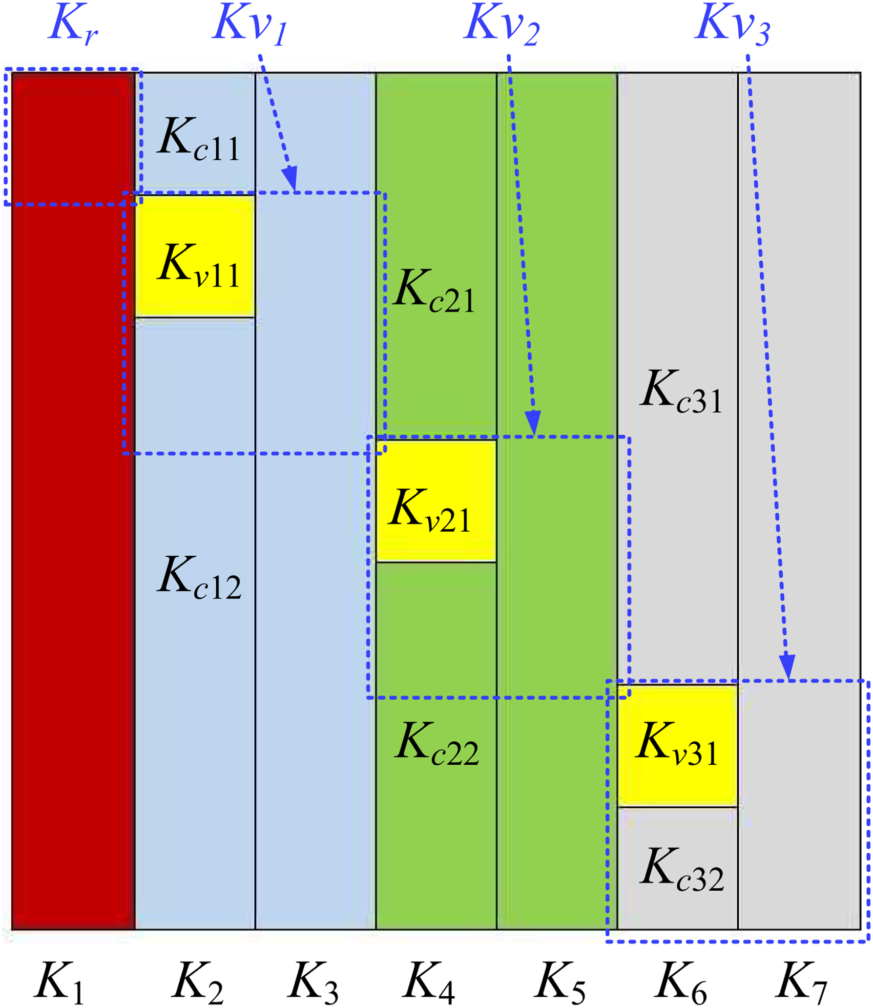

K_r is associated with the shaft, corresponding to the lateral generalized coordinates in two directions and the torsional generalized coordinates, and it is a 14×14 matrix. K_v1, K_v2, and K_v3 are local assembled matrices corresponding to the blades attached to these three disks. Their orders are 15×15, 18×18, and 21×21, respectively.

To facilitate the computation, the assembled stiffness matrix is segmented into seven column matrix blocks K₁–K₇, as shown in Figure 5, and their column numbers are 14, 3, 12, 3, 15, 3, and 18. K₁, K₃, K₅, and K₇ are constant matrices. K₂, K₄, and K₆ contain the nonlinear matrices K_v11, K_v21, and K_v31 of the cracked blade, respectively. Furthermore, K₂ is segmented into K_c11, K_v11, and K_c12, K₄ is segmented into K_c21, K_v21, and K_c22, and K₆ is segmented into K_c31, K_v31, and K_c32.

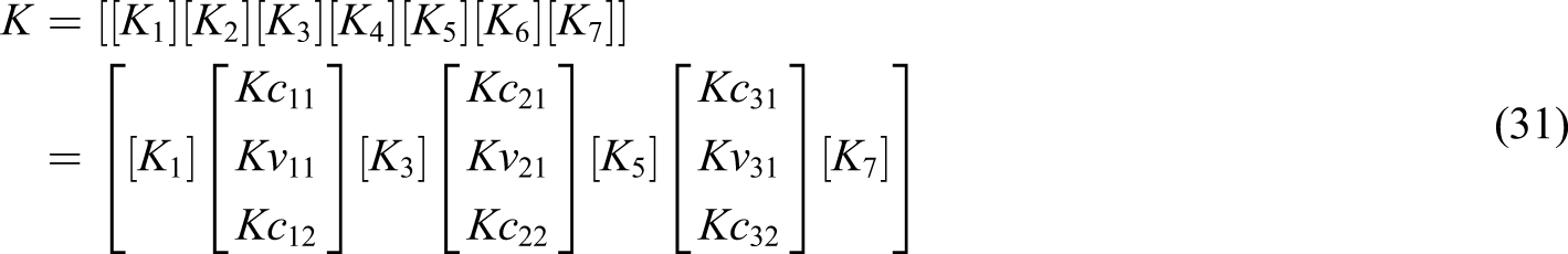
Finally, the assembled stiffness matrix is segmented into 13 matrix blocks, as shown in equation (31). There are only three 3×3 nonlinear matrices, K_v11, K_v21, and K_v31, and the other matrix blocks are constant

\begin{array}{l} K = [[K_{1}] [K_{2}] [K_{3}] [K_{4}] [K_{5}] [K_{6}] [K_{7}]] \\ = [[K_{1}] [\begin{matrix} K c_{11} \\ K v_{11} \\ K c_{12} \end{matrix}] [K_{3}] [\begin{matrix} K c_{21} \\ K v_{21} \\ K c_{22} \end{matrix}] [K_{5}] [\begin{matrix} K c_{31} \\ K v_{31} \\ K c_{32} \end{matrix}] [K_{7}]] \end{array}

(31)

Separation of local nonlinearity

First, the POD transform matrix $V$ , as shown in equation (25), is segmented as follows

V = {[\begin{matrix} V_{1}^{T} & V_{2}^{T} & V_{3}^{T} & V_{4}^{T} & V_{5}^{T} & V_{6}^{T} & V_{7}^{T} \end{matrix}]}^{T}

(32)The orders of the matrix blocks in V correspond to those in the assembled stiffness matrix K, as shown in equation (31). Thus, the matrix blocks are content with matrix operation rules.

Letting ${(V^{T} V)}^{- 1} V^{T} = T_{v}$ , the POD transform of the assembled stiffness matrix, as shown in equation (26), can be rewritten as follows

\begin{array}{l} K_{R} = {(V^{T} V)}^{- 1} V^{T} K V \\ = T_{v} [[K_{1}] [K_{2}] [K_{3}] [K_{4}] [K_{5}] [K_{6}] [K_{7}]] \\ \cdot {[V_{1}^{T} V_{2}^{T} V_{3}^{T} V_{4}^{T} V_{5}^{T} V_{6}^{T} V_{7}^{T}]}^{T} \\ = T_{v} K_{1} V_{1} + T_{v} K_{2} V_{2} + T_{v} K_{3} V_{3} + T_{v} K_{4} V_{4} + T_{v} K_{5} V_{5} + T_{v} K_{6} V_{6} + T_{v} K_{7} V_{7} \end{array}

(33)where

T_{v} K_{1} V_{1}, T_{v} K_{3} V_{3}, T_{v} K_{5} V_{5}, T_{v} K_{7} V_{7}

are constant matrices and can be solved in pretreatment steps.

Denoting $T_{v}$ by $[\begin{matrix} T_{v 11} & T_{v 12} & T_{v 13} \end{matrix}]$ , where $T_{v 11}$ , $T_{v 12}$ , and $T_{v 13}$ satisfy the matrix multiplication rules with $K c_{11}$ , $K v_{11}$ , and $K c_{12}$ . Then, $T_{v} K_{2} V_{2}$ can be reconstructed as given below

T_{v} K_{2} V_{2} = [\begin{matrix} T_{v 11} & T_{v 12} & T_{v 13} \end{matrix}] [\begin{matrix} K c_{11} \\ K v_{11} \\ K c_{12} \end{matrix}] V_{2} = T_{v 11} K c_{11} V_{2} + T_{v 12} K v_{11} V_{2} + T_{v 13} K c_{12} V_{2}

(34)where

T_{v 11} K c_{11} V_{2}

and

T_{v 13} K c_{12} V_{2}

are constant matrices, which can be solved in pretreatment steps.

T_{v 12} K v_{11} V_{2}

is the POD transform of the cracked blade in the first disk, and this operation needs to be implemented at each time step during the iteration. At this point,

K v_{11}

is only a 3×3 matrix, and the computation time of

T_{v 12} K v_{11} V_{2}

is significantly lower than that of

{(V^{T} V)}^{- 1} V^{T} K V

In a similar way, $T_{v}$ is denoted by $[\begin{matrix} T_{v 21} & T_{v 22} & T_{v 23} \end{matrix}]$ , where $T_{v 21}$ , $T_{v 22}$ , and $T_{v 23}$ satisfy the matrix multiplication rules with $K c_{21}$ , $K v_{21}$ , and $K c_{22}$ . Then, $T_{v} K_{4} V_{4}$ can be reconstructed as given below

\begin{array}{l} T_{v} K_{4} V_{4} = [\begin{matrix} T_{v 21} & T_{v 22} & T_{v 23} \end{matrix}] [\begin{matrix} K c_{21} \\ K v_{21} \\ K c_{22} \end{matrix}] V_{4} \\ = T_{v 21} K c_{21} V_{4} + T_{v 22} K v_{21} V_{4} + T_{v 23} K c_{22} V_{4} \end{array}

(35)where only

T_{v 22} K v_{21} V_{4}

needs to be operated during the iteration.

In a similar way, $T_{v} K_{6} V_{6}$ can be reconstructed as follows

\begin{array}{l} T_{v} K_{6} V_{6} = [\begin{matrix} T_{v 31} & T_{v 32} & T_{v 33} \end{matrix}] [\begin{matrix} K c_{31} \\ K v_{31} \\ K c_{32} \end{matrix}] V_{6} \\ = T_{v 31} K c_{31} V_{6} + T_{v 32} K v_{31} V_{6} + T_{v 33} K c_{32} V_{6} \end{array}

(36)where only

T_{v 32} K v_{31} V_{6}

needs to be operated during the iteration.

Consequently, these three 3×3 nonlinear matrices, K_v11, K_v21, and K_v31, are separated from the assembled stiffness matrix under the constraint of POD transformation rules.

Flowcharts of the proposed method

The main innovation of this method is that two key operations, the coordinate transformation and nonlinearity separation, are constructed, such that the POD dimension reduction transformation of the large matrix can be carried out in the pretreatment step. This greatly reduces the calculation amount of POD dimension reduction transformation in the iterative process to realize the efficient solution of time varying and nonlinear equations.

The flowcharts of the proposed method are shown in Figure 6. Compared with Figure 4, the main differences in steps are as follows:

Figure 6.

Flowcharts of the proposed constant coefficients local nonlinearity proper orthogonal decomposition method.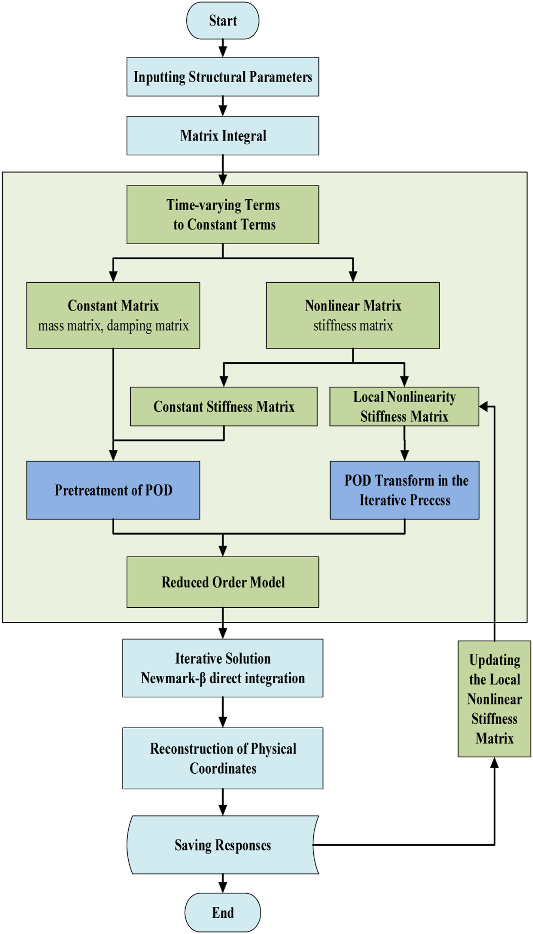

First, the time varying terms are transformed into constant terms by introducing the coordinate transformation and the constructing equation transformation. At this point, the assembled vibration equations only contain a constant mass and damping matrix and a nonlinear stiffness matrix.

Then, matrix segmentation and separation strategies are proposed to separate the local nonlinear stiffness matrix of the cracked blade from the assembly stiffness matrix under the constraint of POD transformation rules. At this point, the assembly nonlinear stiffness matrix is divided into a constant matrix and a local nonlinear matrix.

After that, the POD dimension reduction transformation of the constant mass matrix, damping matrix, and constant stiffness matrix can be implemented in the pretreatment step, which achieves a more efficient POD reduction operation. Only the small-sized local nonlinear stiffness matrix needs to be transformed in the iteration process at each time step.

Finally, the pretreatment and dynamic updated POD transformations are fused to construct the reduced-order model, which can be solved numerically by the Newmark-β method.

Comparison of the results of different solving methods

This section compares the response errors and efficiencies of five models. The original time varying and nonlinear vibration model (equations (37)–(40)) is abbreviated as PC. The POD transformed model of the PC is abbreviated as PC_POD. The constant coefficient model (equations (41)–(44)) is abbreviated as CC. The POD transformed model of the CC is abbreviated as CC_POD. The POD transformed model of the CC adopts the local nonlinear separation strategy, which is the proposed method and is abbreviated as CC_LNLPOD.

The rotation speed of the rotor system is Ω = 2900 r/min and the rotating frequency is 1× = 48.3 Hz. Aerodynamic loads are applied to blades by traveling wave excitation, and the fundamental frequencies are set to 6×, 7×, and 8× at these three stages. An eccentric load is applied to the rotating shaft.

Comparison of the PC and PC_POD

The response error comparisons of the PC_POD models (with different reduction orders) and the original model PC are shown in Figure 7. In this case, the generalized degrees of freedom of the PC is f_d = 68 (the parameter M in equation (25)), and the generalized degrees of freedom of the three PC_POD models are f_rd = 5, f_rd = 15, and f_rd = 25, (the parameter k in equation (25)), respectively.

Figure 7.

Vibration responses of a shaft solved by PC and PC_POD models. (a) Time domain waveforms and (b) frequency spectra. PC_POD: proper orthogonal decomposition transformed model of the PC; PC: periodic coefficients.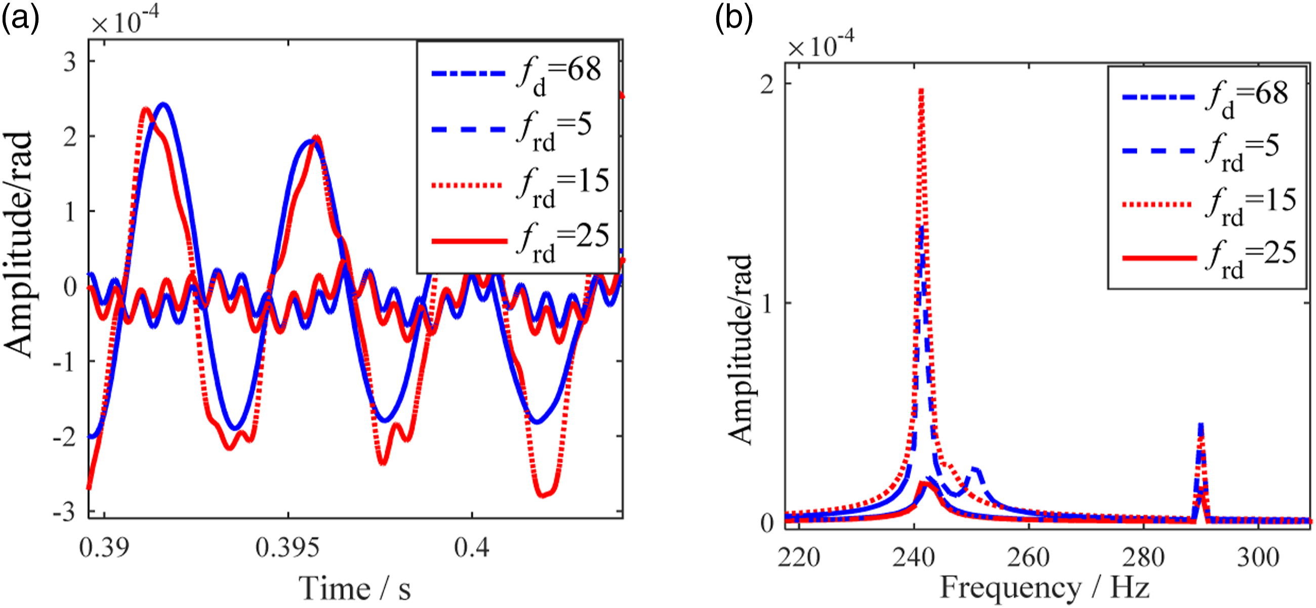

Figure 7 shows that when the generalized degree of freedom is reduced to f_rd = 5 and f_rd = 15, the response amplitudes of the reduced-order models differ greatly from that of the original model f_d = 68. The frequency components and amplitudes of the spectra are also significantly different, which indicates that these two reduced-order models cannot obtain the same precision as the original model.

The time-domain waveform of the model whose order is reduced to f_rd = 25 is almost the same as that of the PC model f_d = 68. In addition, the frequency components and amplitudes of these two models coincide well. This shows that the accuracy of the PC_POD model with DOFs reduced to f_rd = 25 satisfies the requirements of the quantitative and qualitative analysis of vibration responses.

Figure 8 shows the computation time of the four models mentioned above. The solved time history, that is, the duration of the vibration response, is one second. After reducing the order, the solution time of the model can be reduced. The time reductions of low-order models are significant, but the precision of the models when f_rd = 5 and f_rd = 15 cannot meet the accuracy requirements. However, the accuracy of the reduced model when f_rd = 25 satisfies the requirements, but its time reduction is not sufficient.

Figure 8.

Time-consuming comparisons of the PC and PC_PODs. PC_POD: proper orthogonal decomposition transformed model of the PC; PC: periodic coefficients.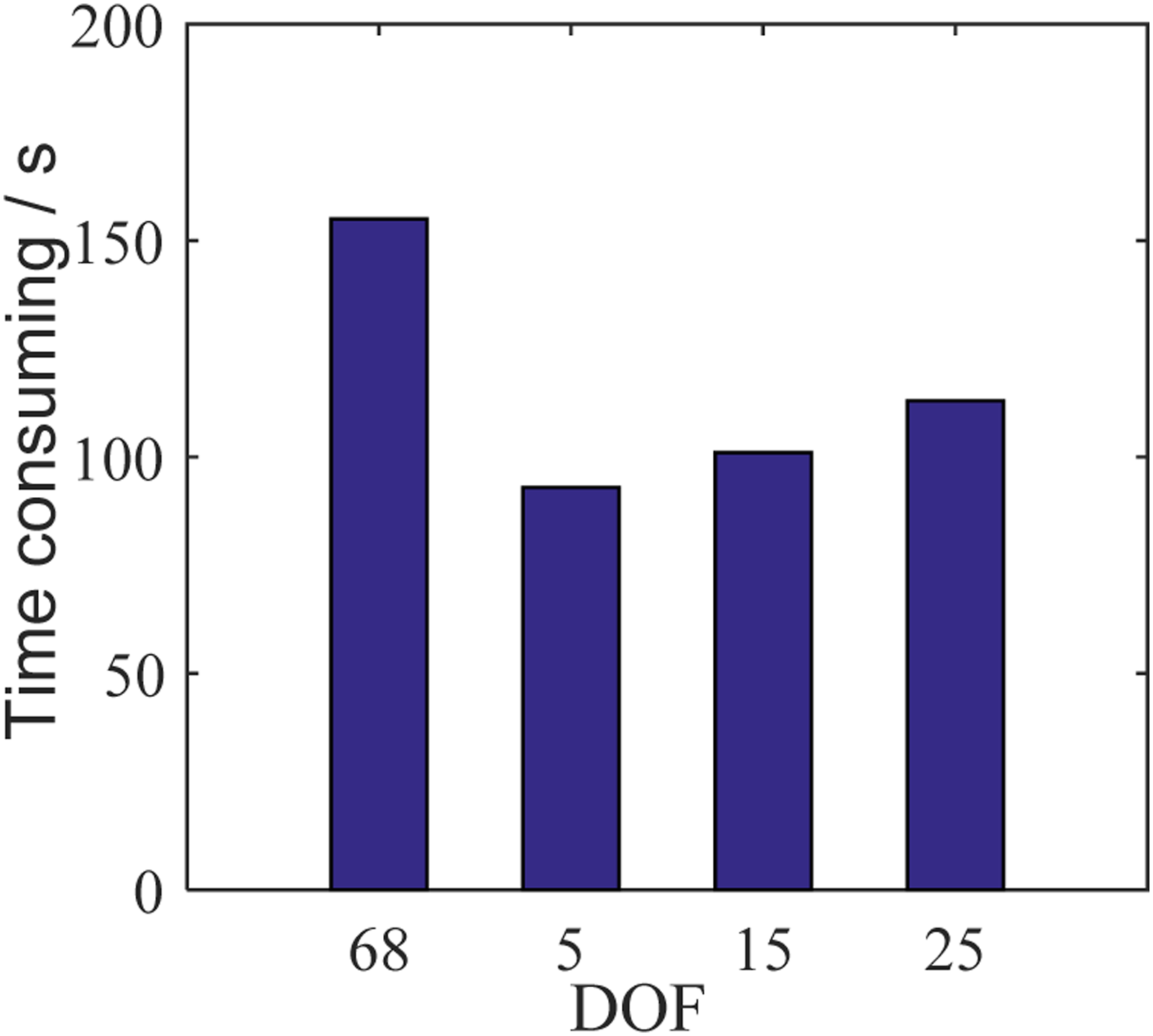

The accuracy and time-consuming comparisons show that it is not a reasonable strategy to directly apply the POD for the periodic coefficient model.

Comparison of the CC versus CC_LNLPOD

The transformation from the time varying equation (periodic coefficient) PC into the CC equation is realized by the variable substitution of the generalized coordinates, which do not involve model reduction. Therefore, the accuracies of the PC and CC are equivalent.

In the CC model, the time varying mass matrix and damping matrix are transformed into a constant matrix so that their POD transformations can be carried out in the pretreatment step, which can significantly reduce the calculation time. However, the assembly stiffness matrix is nonlinear, and its POD transformation needs to be carried out in iterations. The proposed local nonlinearity separation strategy does not change the model orders but optimizes its solution strategy. Therefore, the accuracy of CC_LNLPOD is the same as that of CC_POD.

Therefore, we only compare the accuracies of the CC_LNLPOD and CC models. The orders of the CC_LNLPOD models are reduced to f_rd = 15 and f_rd = 25, and the order of the CC model is f_d = 68. The comparison results of the vibration responses are shown in Figure 9. The solution results of the reduced model CC_LNLPOD when f_rd = 15 are significantly different from those of the original model CC ( f_d = 68), which indicates that the reduced model when f_rd = 15 cannot retain the response characteristics of the original model.

Figure 9.

Comparison of the vibration response of the CC and CC_LNLPODs: (a) torsional responses and (b) lateral responses. CC: constant coefficients; CC_LNLPODs: constant coefficients local nonlinearity proper orthogonal decomposition.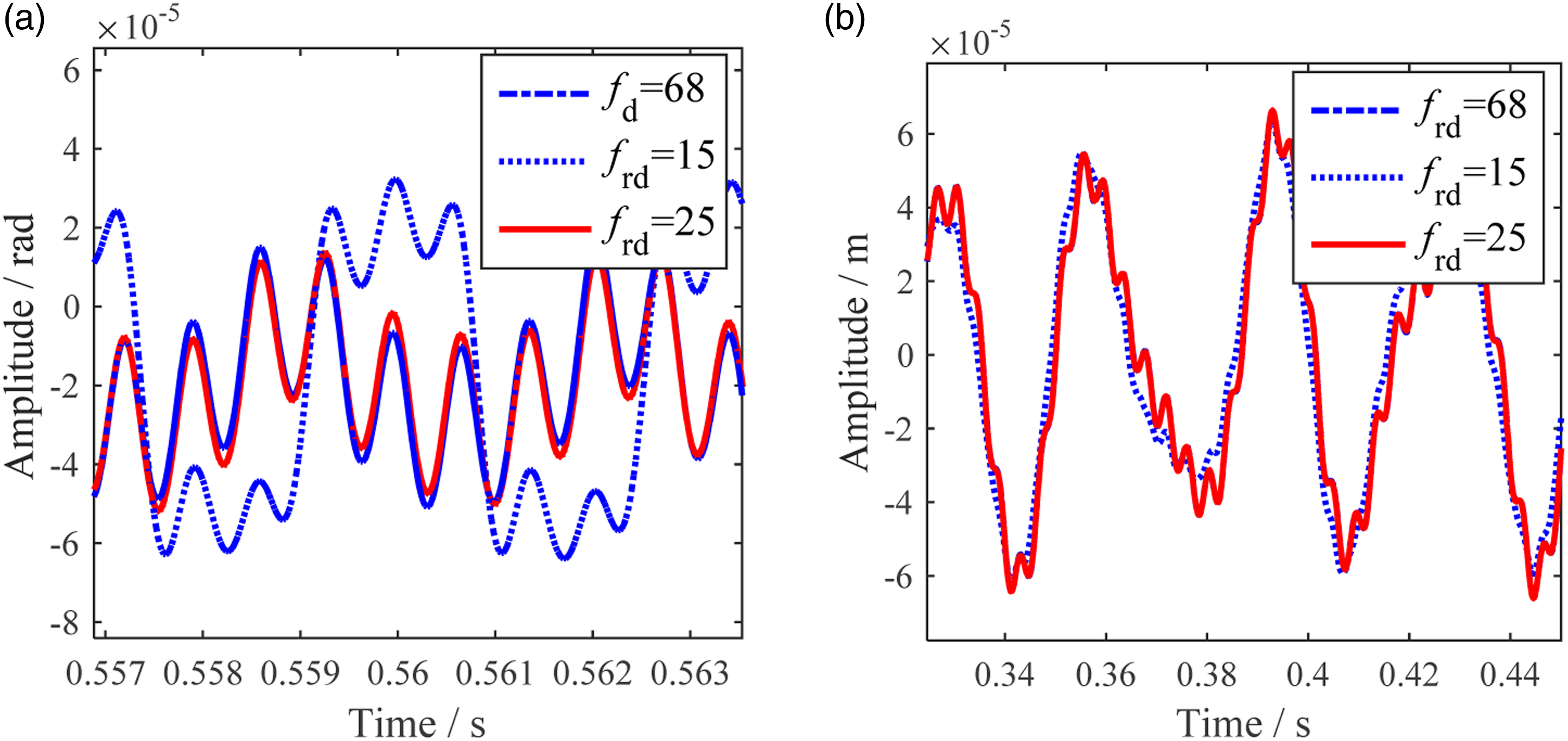

In the reduced-order model CC_LNLPOD when f_rd = 25, the time-domain waveform coincides well with that of the original model CC with f_d = 68. This shows that the accuracy of the CC_LNLPOD model with DOFs reduced to f_rd = 25 satisfies the needs of quantitative and qualitative analysis of vibration responses.

Time consumption comparison

This section compares the time consumption of each model when f_rd = 25. Figure 10 shows the comparisons of the time consumption of the PC, CC, CC_POD, and CC_LNLPOD models when the solved time histories, that is, the durations of the vibration response are 0.5 s, 1 s, and 2 s. Figure 10 shows that constant coefficient transformation, POD transformation, and local nonlinearity separation all have significant effects on reducing the computational time. Compared with the original periodic coefficient model, the computation time of the CC, CC_POD, and CC_NLPOD models decreases significantly with time.

Figure 10.

Time consumption comparisons of the four models.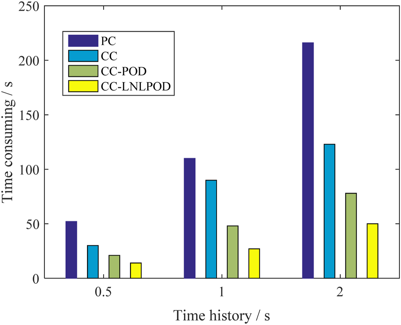

Table 1 compares the time consumptions of the four models for three time histories (0.5 s, 1 s, and 2 s). The time consumptions of the CC model are 57.7%, 81.8%, and 56.9% of that of the original PC model, respectively. Although the solving efficiency is improved, the time-consuming reduction rates are less than 50%. The time consumptions of the CC_POD model are 40.4%, 43.6%, and 36.1% of that of the PC model. The efficiency has been improved again. The time consumption of CC_LNLPOD, in which the constant coefficient transformation and local nonlinearity separation are proposed and adopted, are 26.9%, 24.5%, and 23.1% of that of the original PC model, respectively. The efficiency of the solution is greatly improved, and the time-consuming rate is approximately 1/4 that of the PC model.

Table 1.

Comparison of the time consumption of the four models.

f_d = 68 and f_rd = 25
Time history (s)	Time consumption				Time consumption comparison
Time history (s)	PC (s)	CC (s)	CC_POD (s)	CC_LNLPOD (s)	CC/PC (%)	CC_POD/PC (%)	CC_LNLPOD/PC (%)
0.5	52	30	21	14	57.7	40.4	26.9
1	110	90	48	27	81.8	43.6	24.5
2	216	123	78	50	56.9	36.1	23.1

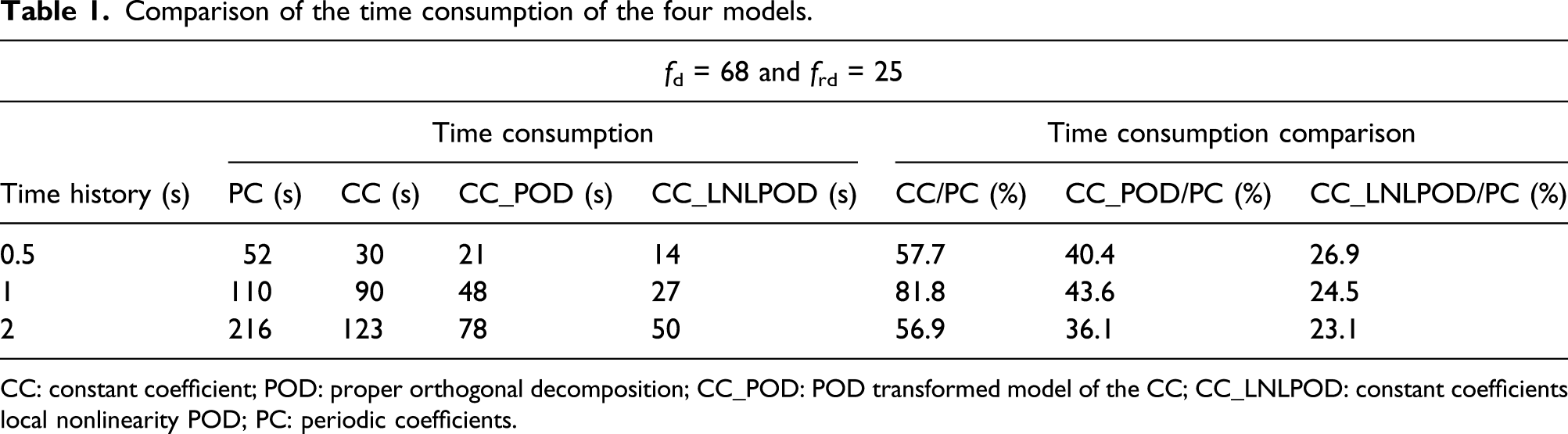
CC: constant coefficient; POD: proper orthogonal decomposition; CC_POD: POD transformed model of the CC; CC_LNLPOD: constant coefficients local nonlinearity POD; PC: periodic coefficients.

The comparison results show that the proposed CC_LNLPOD solution method significantly reduces the computational time, and its accuracy is consistent with that of the original PC model, thereby achieving an efficient solution for the equation with time varying coefficients and nonlinearities.

Conclusions

In this study, an efficient solving method is proposed for the time varying and nonlinear vibration equation of a multistage blade–disk–shaft system. The main contributions of this study are summarized as follows.

Vibration equations are established to illustrate the inevitability of time varying coefficients and nonlinearities in the dynamic models that consider the influence of the centrifugal effect and bending vibration on blade cracks.

By introducing the coordinate transformation and constructing equation transformation, the time varying terms are transformed into constant terms, and the assembled vibration equations only contain a constant mass matrix, constant damping matrix, and nonlinear stiffness matrix.

Matrix segmentation and separation strategies are proposed to separate the local nonlinear stiffness matrix of the cracked blade under the constraint of POD transformation rules. In addition, the assembly of the nonlinear stiffness matrix is divided into a constant matrix and a local nonlinear matrix.

After the transformation of the time varying terms and the separation of the local nonlinear terms, the POD dimension reduction transformation of the assembled matrix can be carried out in the pretreatment step, which greatly reduces the calculation time.

The comparison results show that, on the premise of ensuring the solution accuracy, the time-consuming rate of the proposed method is approximately 1/4 of that of the conventional method.

Footnotes

Declaration of conflicting interests

The author(s) declared no potential conflicts of interest with respect to the research, authorship, and/or publication of this article.

Funding

The author(s) disclosed receipt of the following financial support for the research, authorship, and/or publication of this article: This work was supported by the National Natural Science Foundation of China (No. 51905399) and the Scientific Research Starting Foundation of Central South University (No. 202044013).

ORCID iD

Jingsong Xie

Appendix 1. Time varying vibration equations

(37)

( M x + ∑ j − 1 n ( M d x z d j + M d x d z d j + 1 2 M v x d z d j + M v x z d j ) ) q ¨ x + C x q ˙ x + ( K x − Ω 2 ∑ j − 1 n M d x d z d j − 1 2 Ω 2 ∑ j − 1 n M v x d z d j ) q x − sin ( Ω t ) ∑ j = 1 n M x ϕ j q ¨ ϕ + ( Ω ∑ j − 1 n ( 2 M d x d z d j + M v x d z d j ) ) q ˙ y − ∑ j − 1 n ∑ i − 0 N j − 1 ( ( sin ( Ω t + θ b i ) M v x z d v j + cos ( Ω t + θ b i ) M v x d z d v j ) q ¨ v j i + 2 Ω ( cos ( Ω t + θ b i ) ) M v x z d v j q ˙ v j i − Ω 2 ⁡ sin ( Ω t + θ b i ) ( M v x z d v j ) q v j i )

where n–number of disk, n = 3, j–serial number of the disks, N_j–number of blades in the j^th disk, i–serial number of the blades, M x = ρ s A s ∫ 0 s U U T d z , K x = E s I s x ∫ 0 s ( ∂ 2 U / ∂ z 2 ) ( ∂ 2 U T / ∂ z 2 ) d z , M d x z d = ρ d h d π ( r 2 2 − r 1 2 ) U U T | z d , M d x d z d = ( 1 / 4 ) ρ d h d π ( r 2 4 − r 1 4 ) ( ∂ U / ∂ z ) ( ∂ U T / ∂ z ) | z d , M v x d z d = ρ b A b ( ( 1 / 3 ) L 3 + r 2 L 2 + r 2 2 L ) N ( ∂ U / ∂ z ) ( ∂ U T / ∂ z ) | z d , M v x d z d v = ρ b A b sin ( β b ) ∂ U / ∂ z | z d ∫ 0 L ( l + r 2 ) V T d l , M v x z d = ρ b A b L N U U T | z d , M v x z d v = ρ b A b cos ( β b ) U | z d ∫ 0 L V T d l , C x = α M x + β K x , M x ϕ = m e e ∫ 0 s U ( z ) δ ( z − z d ) Φ T ( z d ) d z = m e e U ( z d ) Φ T ( z d ) (38)

( M y + ∑ j − 1 n ( M d y z d j + M d y d z d j + 1 2 M v y d z d j + M v y z d j ) ) q ¨ y + C y q ˙ y + ( K y − Ω 2 ∑ j − 1 n M d y d z d j − 1 2 Ω 2 ∑ j − 1 n M v y d z d j ) q y + cos ( Ω t ) ∑ j = 1 n M y ϕ j q ¨ ϕ − ( Ω ∑ j − 1 n ( 2 M d y d z d j + M v y d z d j ) ) q ˙ x + ∑ j − 1 n ∑ i − 0 N j − 1 ( ( + cos ( Ω t + θ b i ) M v y z d v j − sin ( Ω t + θ b i ) M v y d z d v j ) q ¨ v j i − 2 Ω ( sin ( Ω t + θ b i ) ) M v y z d v j q ˙ v j i − Ω 2 ⁡ cos ( Ω t + θ b i ) ( M v y z d v j ) q v j i ) = Q y

where M y = ρ s A s ∫ 0 s U U T d z , K y = E s I s x ∫ 0 s ∂ 2 U ∂ z 2 ∂ 2 U T ∂ z 2 d z , M d y d z d = 1 4 ρ d h d π ( r 2 4 − r 1 4 ) ∂ U ∂ z ∂ U T ∂ z | z d , M v y d z d v = ρ b A b ⁡ sin ( β b ) ∂ U ∂ z | z d ∫ 0 L ( l + r 2 ) V T d l , M v y z d = ρ b A b L N U U T | z d , M v y z d v = ρ b A b ⁡ cos ( β b ) U | z d ∫ 0 L V T d l , C y = α M y + β K y , M y ϕ = m e e ∫ 0 s U T ( z ) δ ( z − z d ) Φ ( z d ) d z = m e e U T ( z d ) Φ ( z d ) (39)

( M ϕ + ∑ j − 1 n M d ϕ z d j + ∑ j − 1 n M v ϕ z d j ) q ¨ ϕ + C ϕ q ˙ ϕ + ( K ϕ − Ω 2 ∑ j − 1 n M d ϕ z d j − Ω 2 ∑ j − 1 n M v ϕ z d j ) q ϕ − sin ( Ω t ) ∑ j = 1 n M ϕ x y j q ¨ x + cos ( Ω t ) ∑ j = 1 n M ϕ x y j q ¨ y + ∑ j = 1 n ∑ i = 0 N j − 1 ( M v ϕ z d v j q ¨ v j i − Ω 2 M v ϕ z d v j q v j i ) = Q ϕ

where M ϕ = ρ s I s p ∫ 0 s Φ Φ Τ d z , K ϕ = G s I s p ∫ 0 s ( ∂ Φ / ∂ z ) ( ∂ Φ T / ∂ z ) d z , M d ϕ z d = 1 2 ρ d h d π ( r 2 4 − r 1 4 ) Φ Φ Τ | z d , M v ϕ z d = ρ b A b N ( 1 3 L 3 + r 2 L 2 + r 2 2 L ) Φ Φ T | z d , M v ϕ z d v = ρ b A b ⁡ cos ( β b ) Φ | z d ∫ 0 L ( l + r 2 ) V T d l , C ϕ = α M ϕ + β K ϕ , M ϕ x y = m e e ∫ 0 s Φ ( z − z d ) U T ( z d ) d z = m e e ( z d ) U T ( z d ) (40)

M v j q ¨ v j + C v j q ˙ v j + ( K v j − cos 2 ( β ) Ω 2 M v j + 1 2 Ω 2 ( K Ω j + K Ω j T ) + 2 K cp j ) q v j − K cp j q v j ( i + 1 ) − K cp j q v j ( i − 1 ) ( − cos ( Ω t + θ b i ) M s v d z d s j T − sin ( Ω t + θ b i ) M s d v z d s j T ) q ¨ x + ( 2 Ω sin ( Ω t + θ b i ) M s v d z d s j T ) q ˙ x + ( Ω 2 cos ( Ω t + θ b i ) M s v d z d s j T ) q x ( − sin ( Ω t + θ b i ) M s v d z d s j T + cos ( Ω t + θ b i ) M s d v z d s j T ) q ¨ y ( − 2 Ω cos ( Ω t + θ b i ) M s v d z d s j T ) q ˙ y + ( Ω 2 ⁡ sin ( Ω t + θ b i ) M s v d z d s j T ) q y + M ϕ d v z d ϕ j T q ¨ ϕ − Ω 2 M ϕ d v z d ϕ j T q ϕ = Q v j

where M v = ρ b A b ∫ 0 L V V T d l , M s v d z d s = ρ b A b ⁡ sin ( β b ) ∂ U ∂ z | z d ∫ 0 L ( l + r 2 ) V T d l , M s d v z d s = ρ b A b ⁡ cos ( β b ) U | z d ∫ 0 L V T d l , M ϕ d v z d ϕ = ρ b A b ⁡ cos ( β b ) Φ | z d ∫ 0 L ( l + r 2 ) V T d l , K v = E I ∫ 0 L ∂ 2 V ∂ l 2 ∂ 2 V T ∂ l 2 d l , K Ω = 1 2 ρ A b ∫ 0 L [ ( r 2 + L ) 2 − ( r 2 + l ) 2 ] ∂ V ∂ l ∂ V T ∂ l d l , K cp = ∫ 0 L k cp ( l ) ( ∂ V ∂ l ∂ V T ∂ l ) d l , C v = α M v + β K v

Appendix 2. Constant coefficient vibration equations

(41)

( M x + ∑ j = 1 n ( M d x z d j + M d x d z d j + 1 2 M v x d z d j + M v x z d j ) ) q ¨ x ¯ + C x q ˙ x ¯ + ( K x − Ω 2 M x − Ω 2 ∑ j − 1 n ( M d x z d j + M v x z d j ) ) q x ¯ − 2 Ω ( M x + ∑ j − 1 n ( M d x z d j + M v x z d j ) ) q ˙ y ¯ − Ω C x q y ¯ − ∑ j = 1 n ∑ i = 0 N j − 1 ( ( sin ( θ b i ) M v x z d v j + cos ( θ b i ) M v x d z d v j ) q ¨ v j i + 2 Ω ⁡ cos ( θ b i ) M v x z d v j q ˙ v j i − Ω 2 ⁡ sin ( θ b i ) ( M v x z d v j ) q v j i ) = cos ( Ω t ) Q x + sin ( Ω t ) Q y

(42)

( M y + ∑ j − 1 n ( M d y z d j + M d y d z d j + 1 2 M v y d z d j + M v y z d j ) ) q ¨ y ¯ + C y q ˙ y ¯ + ( K y − Ω 2 M y − Ω 2 ∑ j = 1 n ( M d y z d j + M v y z d j ) ) q y ¯ + ∑ j − 1 n M y ϕ j q ¨ ϕ + 2 Ω ( M y + ∑ j = 1 n ( M d y z d j + M v y z d j ) ) q ˙ x ¯ + Ω C y q x ¯ + ∑ j = 1 n ∑ i = 0 N j − 1 ( ( + cos ( θ b i ) M v y z d v j − sin ( θ b i ) M v y d z d v j ) q ¨ v j i − 2 Ω ( sin ( θ b i ) ) M v y z d v j q ˙ v j i − Ω 2 ⁡ cos ( θ b i ) ( M v y z d v j ) q v j i ) = − sin ( Ω t ) Q x + cos ( Ω t ) Q y

(43)

( M ϕ + ∑ j = 1 n M d ϕ z d j + ∑ j = 1 n M v ϕ z d j ) q ¨ ϕ + C ϕ q ˙ ϕ + ( K ϕ + Ω 2 ∑ j = 1 n M d ϕ z d j − Ω 2 ∑ j = 1 n M v ϕ z d j ) q ϕ + ∑ j − 1 n M ϕ x y j ( - q ¨ y ¯ + 2 Ω q ˙ x ¯ + Ω 2 q y ¯ ) + ∑ j = 1 n ∑ i = 0 N j − 1 ( M v ϕ z d v j q ¨ v j i − Ω 2 M v ϕ z d v j q v j i ) = Q ϕ

(44)

M v j q ¨ v j + C v j q ˙ v j + ( K v j − cos 2 ( β ) Ω 2 M v j + 1 2 Ω 2 ( K Ω j + K Ω j T ) + 2 K cp j ) q v j − K cp j q v j ( i + 1 ) − K cp j q v j ( i − 1 ) ( − cos ( θ b i ) M s v d z d s j T − sin ( θ b i ) M s d v z d s j T ) q ¨ x ¯ + ( 2 Ω ⁡ cos ( θ b i ) M s v d z d s j T ) q ˙ x ¯ + ( Ω 2 ⁡ sin ( θ b i ) M s v d z d s j T ) q x ¯ ( − sin ( θ b i ) M s v d z d s j T + cos ⁡ θ b i ( θ b i ) M s d v z d s j T ) q ¨ y ¯ + ( 2 Ω ⁡ sin ( θ b i ) M s v d z d s j T ) q ˙ y ¯ − ( Ω 2 ⁡ cos ( θ b i ) M s v d z d s j T ) q y ¯ + M ϕ d v z d ϕ j T q ¨ ϕ − Ω 2 M ϕ d v z d ϕ j T q ϕ = Q v j

References

Kim

Hong

J-G

Chung

. Nonlinear dynamic modeling and response analysis of a rotor-blade system with whirling motion. Nonlinear Dyn 2019; 98: 953–970.

Rzadkowski

. Dynamic multi-stage analysis of a mistuned aircraft rotor with foreign object ingestion. J Vib Eng Tech 2018; 6: 339–355.

Yin

, et al. Nonlinear vibration response analysis of a rotor-blade system with blade-tip rubbing. Nonlinear Dyn 2016; 84: 1225–1258.

She

Tang

, et al. The effect of blade vibration on the nonlinear characteristics of rotor-bearing system supported by nonlinear suspension. Nonlinear Dyn 2017; 89: 987–1010.

Ghannad

Morteza

. Vibration mitigation of a flexible bladed rotor dynamic system with passive dynamic absorbers. Commun Nonlinear 2019; 69: 1–30.

Anjum

J-H

. Analysis of nonlinear vibration of nano/microelectromechanical system switch induced by electromagnetic force under zero initial conditions. Alexandria Eng J 2020; 59: 4343–4352.

Akuro

Chinwuba

. Analysis of the coupled nonlinear vibration of a two-mass system. J Appl Comput Mech 2019; 5: 935–950.

Skrzypacz

Zhang

, et al. Approximate periodic solutions to microelectromechanical system oscillator subject to magnetostatic excitation. Math Meth Appl Sci 2020. DOI:10.1002/mma.7018

Noeiaghdam

Dreglea

, et al. Error estimation of the homotopy perturbation method to solve second kind volterra integral equations with piecewise smooth kernels: application of the CADNA Library. Symmetry 2020; 12: 1730.

10.

El‐Dib

. The reducing rank method to solve third‐order Duffing equation with the homotopy perturbation. Numer Methods Partial Differ Equ 2021; 37: 1800–1808.

11.

Biswal

Chakraverty

Ojha

. Application of homotopy perturbation method in inverse analysis of Jeffery-Hamel flow problem. Eur J Mech B Fluid 2020; 86: 107–112.

12.

T-T

Zheng

W-Q

. Adomian decomposition method for first order PDEs with unprescribed data. Alexandria Eng J 2021; 60: 2563–2572.

13.

Lichae

Biaza

Ayati

. Asymptotic decomposition method for fractional order Riccati differential equation. Comput Methods Differential Eqs 2021; 9: 63–78.

14.

Bavi

Hajnayeb

Sedighi

H M

. Comments on “Nonlinear phenomena, bifurcations, and routes to chaos in an asymmetrically supported rotor–stator contact system” by Philip Varney and Itzhak Green [J. Sound Vib. 336(2015) 207–226]. J Sound Vib 2017; 409:336–342.

15.

Fang

Zhan

. High order explicit exponential Runge-Kutta methods for semilinear delay differential equations. J Comput Appl Math 2021; 388: 113279.

16.

Vermeire

Hedayati Nasab

. Accelerated implicit-explicit Runge-Kutta schemes for locally stiff systems. J Comput Phys 2021; 429: 110022.

17.

Akbas

. Forced vibration responses of axially functionally graded beams by using ritz method. J Appl Comput Mech 2021; 7: 109–115.

18.

Liu

Hao

, et al. Free vibration and transient dynamic response of functionally graded sandwich plates with power-law nonhomogeneity by the scaled boundary finite element method. Comp Methods Appl Mech Eng 2021; 376: 113665.

19.

Wang

Qian

, et al. Effects of unbalance on the nonlinear dynamics of rotors with transverse cracks. Nonlinear Dyn 2018; 91: 2755–2772.

20.

Pourkiaee

Zucca

. A reduced order model for nonlinear dynamics of mistuned bladed disks with shroud friction contacts. J Eng Gas Turb Power 2019; 141: 1–13.

21.

Joannin

Thouverez

Chouvion

. Reduced-order modelling using nonlinear modes and triple nonlinear modal synthesis. Comput Structures 2018; 203: 18–33.

22.

Sun

Chen

Hou

. Nonlinear dynamical behaviors of a complicated dual-rotor aero-engine with rub-impact. Archive Appl Mech 2018; 88: 1305–1324.

23.

Alsaleh

Sedighi

Ouakad

. Experimental and theoretical investigations of the lateral vibrations of an unbalanced Jeffcott rotor. Front Struct Civil Eng 2020; 14: 1024–1032.

24.

Vergari

Cammi

Lorenzi

. Reduced order modeling approach for parametrized thermal-hydraulics problems: inclusion of the energy equation in the POD-FV-ROM method. Prog Nucl Energ 2020; 118: 103071.

25.

Chen

Y-s

Cao

Q-j

. Bifurcation analysis for nonlinear multi-degree-of-freedom rotor system with liquid-film lubricated bearings. Appl Math Mech 2013; 34: 777–790.

26.

Kim

Cho

. Reduction process based on proper orthogonal decomposition for dual formulation of dynamic substructures. Comput Mech 2019; 64: 1237–1257.

27.

Chen

, et al. A modified nonlinear POD method for order reduction based on transient time series. Nonlinear Dyn 2015; 79: 1195–1206.

28.

Sidhu

Narasingam

Siddhamshetty

, et al. Model order reduction of nonlinear parabolic PDE systems with moving boundaries using sparse proper orthogonal decomposition: application to hydraulic fracturing. Comput Chem Eng 2018; 112: 92–100.

29.

Nguyen

Tran

SBQ

Khan

, et al. POD-DEIM model order reduction technique for model predictive control in continuous chemical processing. Comput Chem Eng 2020; 133: 106638.

30.

Jin

Hou

, et al. An adaptive proper orthogonal decomposition method for model order reduction of multi-disc rotor system. J Sound Vib 2017; 411: 210–231.

31.

Eftekhar Azam

Mariani

Attari

NKA

. Online damage detection via a synergy of proper orthogonal decomposition and recursive Bayesian filters. Nonlinear Dyn 2017; 89: 1489–1511.

32.

Luo

. Design optimization of the last stage of a 4.5-stage compressor using a POD-based hybrid model. Aerospace Sci Tech 2018; 76: 303–314.

33.

Chiu

Huang

. The influence of a cracked blade on rotor’s free vibration. J Vib Acoust 2008; 130: 054502.

34.

M-C

Huang

S-C

. On the vibration of a cracked rotating blade. Shock Vib 1998; 5: 317–323.

35.

Xie

Zhang

, et al. A novel vibration modeling method for a rotating blade with breathing cracks. Sci China Technol Sci 2018; 62: 333–348.

36.

Huang

Kuang

. Effect of a local crack on the dynamic characteristics of a rotating grouped blade disc. Proc Inst Mech Eng C J Mechan 2002; 216: 447–457.

37.

Davidson

. The Newmark-β time-stepping algorithm. In: Computational electromagnetics for RF and microwave engineering. Cambridge: Cambridge University Press, 2005, pp.392–394.

An efficient method for vibration equations with time varying coefficients and nonlinearities

Abstract

Keywords

Introduction

Dynamic model of a multistage blade–disk–shaft system

Modeling of a normal system

Multistage blade–disk–shaft system with a cracked blade

Conventional solution for time varying and nonlinear equations

Proposed CC_LNLPOD method

Nonlinear transient POD

Time varying terms to constant terms

Separation of local nonlinearity

Segmentation of the assembled stiffness matrix

Separation of local nonlinearity

Flowcharts of the proposed method

Comparison of the results of different solving methods

Comparison of the PC and PC_POD

Comparison of the CC versus CC_LNLPOD

Time consumption comparison

Conclusions

Footnotes

Declaration of conflicting interests

Funding

ORCID iD

Appendix 1. Time varying vibration equations

Appendix 2. Constant coefficient vibration equations

References