Numerical solution of a class of space fractional nonlinear vibration equations with periodic boundary conditions by the Fourier spectral method

Abstract

Nonlinear vibration arises everywhere in engineering. So far there is no method to track the exact trajectory of a space fractional nonlinear oscillator; therefore, a sophisticated numerical method is much needed to elucidate its basic properties. For this purpose, a numerical method that combines the Fourier spectral method with the Runge–Kutta method is proposed. Its accuracy and efficiency have been demonstrated numerically. This approach has full physical understanding and numerical access; thus, it can be used to solve many types of nonlinear space fractional partial differential equations with periodic boundary conditions.

Introduction

In engineering, a fast estimation of the periodic property of a nonlinear oscillator is much needed. As an exact solution might be too complex to be used for a practical application, many analytical and numerical methods have been used in open literature, for example, the homotopy perturbation method,^1-4 the barycentric interpolation collocation method,^5-6 the variational iteration method,^7-11 and the reproducing kernel method^12-16 which are still under development and many modifications were proposed to improve the accuracy.

During the past decades, fractional calculus has been playing more and more important roles in fields of science and engineering.^17,18 Many researchers have devoted great energy to study the theory and computation for fractional equations^19-25 and fractal vibration systems.^26-30 In the study, we consider the following space fractional nonlinear vibration equation^31-34

$$u_t+\epsilon u{u}_x+{\alpha }_1{u}^2{u}_x+{\alpha }_2{u}_{xxx}+{\alpha }_3{D}_x^{\beta }u+{\alpha }_{4}f\left(x,t\right)=0,x\in \mathrm{\Omega },t\in \left[0,T\right]$$

(1)

subject to the initial condition given by u(x, 0) = u₀(x), x ∈ Ω ⊂ R, with homogeneous periodic Dirichlet or Neumann boundary conditions, ɛ, α₁, α₂, α₃,α₄, and β are positive parameters, and f represents the nonlinear reaction term.

For ∀ r > 0, let H ^r (Ω) = W^r,2(Ω) be Sobolev space with norm ‖ ⋅‖ and semi-norm |⋅|. Define $H_p^r\left(\mathrm{\Omega }\right)$ as subspace composed by periodic functions with period L on H ^r (Ω), and $H_p^r\left(\mathrm{\Omega }\right)=\left\{u|u\in H^r,u\left(x-L/2\right)=u\left(x+L/2\right)\right\}$ . $u\left(x,t\right)\in H_p^r\left(\mathrm{\Omega }\right)$ , $D_x^{\beta }u$ indicates that β is the Caputo fractional derivative defined of u(x, t) about x, respectively.

Definition 1.1

The β-order Caputo derivative of u(x, t) about x is defined as

$$D_x^{\beta }u\left(x,t\right)=\{\begin{array}{l}\frac{1}{\mathrm{\Gamma }\left(n-\beta \right)}{\displaystyle {\int }_{-\infty }^x{\left(x-\tau \right)}^{n-\beta -1}}\frac{{\partial }^{n}u\left(x,\tau \right)}{\partial {\tau }^n}d\tau ,\hspace{1em}n-1<\beta <n\hfill \\ \frac{{\partial }^{n}u\left(x,t\right)}{\partial t^n},\hspace{1em}\beta =n\in N\hfill \end{array}$$

(2)

Based on (2)

$$F\left[D_x^{\beta }u\left(x,t\right)\right]={\left(i\omega \right)}^{\beta }\widehat{u}\left(\omega ,t\right)$$

(3)

where the Fourier transform and inverse Fourier transform of function u(x, t) about t definition as

$$\widehat{u}\left(\omega ,t\right)=F\left[u\left(x,t\right)\right]={\displaystyle {\int }_{-\infty }^{\infty }u\left(x,t\right)e^{-i\omega x}dx},\hspace{1em}u\left(x,t\right)=F^{-1}\left[\widehat{u}\left(\omega ,t\right)\right]=\frac{1}{2\pi }{\displaystyle {\int }_{-\infty }^{\infty }\widehat{u}\left(\omega ,t\right)e^{i\omega x}d\omega }$$

(4)

Algorithms

Let $\mathrm{\Omega }=\left[-L/2,L/2\right]$ and ⟨u, v⟩ = ∫_Ωuvdx, ‖u‖ = ⟨u, u⟩. For the purpose of spatial discretization, we divide the interval $\left[-L/2,L/2\right]$ into even number N subintervals with spatial steps $h=L/N$ , let x _j = jh, $u_j=u\left(x_j,t\right),j=-N/2,-N/2+1,\dots ,\mathrm{0,1},\dots N/2-1$ .

First, applying the discrete Fourier transform with respect to the spatial variable x, equation (1) can be turned into the semi-discrete scheme (5)

$$\frac{d\widehat{u}}{dt}=-\epsilon F\left\{F^{-1}\left[\widehat{u}\right]\cdot F^{-1}\left[i\omega \widehat{u}\right]\right\}-{\alpha }_{1}F\left\{{\left|F^{-1}\left[\widehat{u}\right]\right|}^2\cdot F^{-1}\left[i\omega \widehat{u}\right]\right\}-{\alpha }_2{\left(i\omega \right)}^3\widehat{u}-{\alpha }_3{\left(i\omega \right)}^{\beta }\widehat{u}-{\alpha }_{4}F\left[f\left(x,t\right)\right]$$

(5)

where $\widehat{u}$ is the discrete Fourier transform of u in spatial direction. The inverse discrete Fourier transform is noted $u=F^{-1}\left[\widehat{u}\right]$ .

Noting $g\left(t,\widehat{u}\right)=-\epsilon F\left\{F^{-1}\left[\widehat{u}\right]\cdot F^{-1}\left[i\omega \widehat{u}\right]\right\}-{\alpha }_{1}F\left\{{\left|F^{-1}\left[\widehat{u}\right]\right|}^2\cdot F^{-1}\left[i\omega \widehat{u}\right]\right\}-{\alpha }_2{\left(i\omega \right)}^3\widehat{u}-{\alpha }_3{\left(i\omega \right)}^{\beta }\widehat{u}-{\alpha }_{4}F\left[f\left(x,t\right)\right]$ . Equation (5) can be transformed into the following form

$$\begin{array}{c}\{\begin{array}{l}{\widehat{u}}_t=g\left(t,\widehat{u}\right)\hfill \\ \widehat{u}\left(\omega ,0\right)=\widehat{u_0}\hfill \end{array}\end{array}$$

(6)

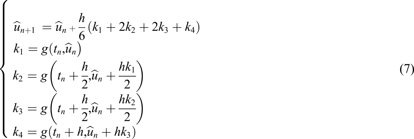
Second, we use the fourth-order Runge–Kutta method to solve the scheme (5), so we can get the solution of equation (1) by using inverse discrete Fourier transform. The fourth-order Runge–Kutta method is the following form

$$\begin{array}{c}\{\begin{array}{l}{\widehat{u}}_{n+1}={\widehat{u}}_n+\frac{h}{6}\left(k_1+2k_2+2k_3+k_4\right)\hfill \\ k_1=g\left(t_n,{\widehat{u}}_n\right)\hfill \\ k_2=g\left(t_n+\frac{h}{2},{\widehat{u}}_n+\frac{h{k}_1}{2}\right)\hfill \\ k_3=g\left(t_n+\frac{h}{2},{\widehat{u}}_n+\frac{h{k}_2}{2}\right)\hfill \\ k_4=g\left(t_n+h,{\widehat{u}}_n+h{k}_3\right)\hfill \end{array}\end{array}$$

(7)

Algorithm is as follows:

Algorithm

Input: L; N; T, M; t = 0: T/M: T; x = L/N∗[−N/2: N/2−1]; k = 2∗pi/L∗[0: N/2−1−N/2: −1]; u = u₀(x.)

Defining KDV.m file, function dut=KDV(t,ut,dummy,k,x)

 u = u₀(x.); ut = fft(u); u = ifft(ut)

 dut = −ɛ∗ fft(u. ∗ ifft(i ∗ k. ∗ ut)) − α₁ ∗ fft(u. ∗ u. ∗ ifft(i ∗ k. ∗ ut))

    − α₂ ∗ (i ∗ k).³ ∗ ut − α₃ ∗ (i ∗ k). ^β ∗ ut − α₄ ∗ fft(f(x., t.))

Using Runge–Kutta method, $\left[t,utsol\right]=ode45\left({}^{\prime }KD{V}^{\prime },t,ut,\left[\right],k\right)$

Output: u _num = ifft(utsol, [], 2)

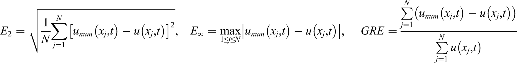
Besides, the validation of our work is confirmed by comparing the analytical solutions and the numerical solutions. The root-mean-square error E₂, the max error E _∞ , the global relative error GRE, and absolute error are used to measure the accuracy of our method

$$E_2=\sqrt{\frac{1}{N}{{\displaystyle \sum _{j=1}^N\left[u_{num}\left(x_j,t\right)-u\left(x_j,t\right)\right]}}^2},\hspace{1em}{E}_{\infty }=\underset{1\le j\le N}{\max }\left|u_{num}\left(x_j,t\right)-u\left(x_j,t\right)\right|, \hspace{1em}GRE=\frac{{\displaystyle \sum _{j=1}^N\left(u_{num}\left(x_j,t\right)-u\left(x_j,t\right)\right)}}{{\displaystyle \sum _{j=1}^{N}u\left(x_j,t\right)}}$$

u _num (x _j , t) and u(x _j , t) are the numerical solution and the analytical solution, respectively, and N is the number of grid points.

Numerical simulations

In this section, following the guidance of the discussions in Numerical simulations, we will select appropriate free parameters and present some numerical simulations for preceding cases, which implies that our current method is a satisfactory and efficient algorithm.

Example 1

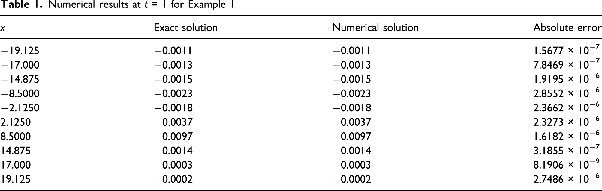
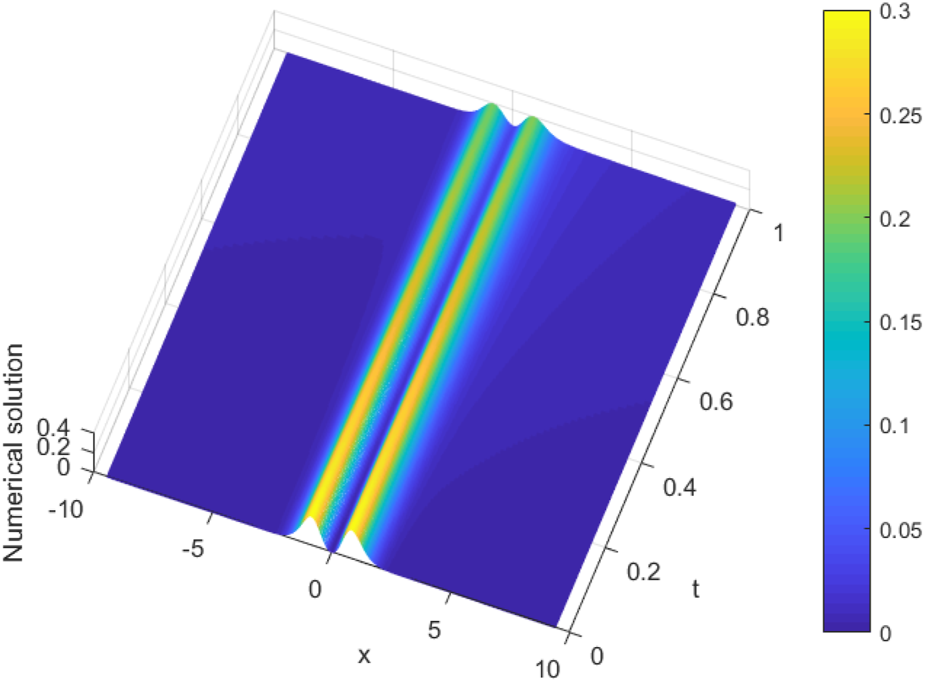
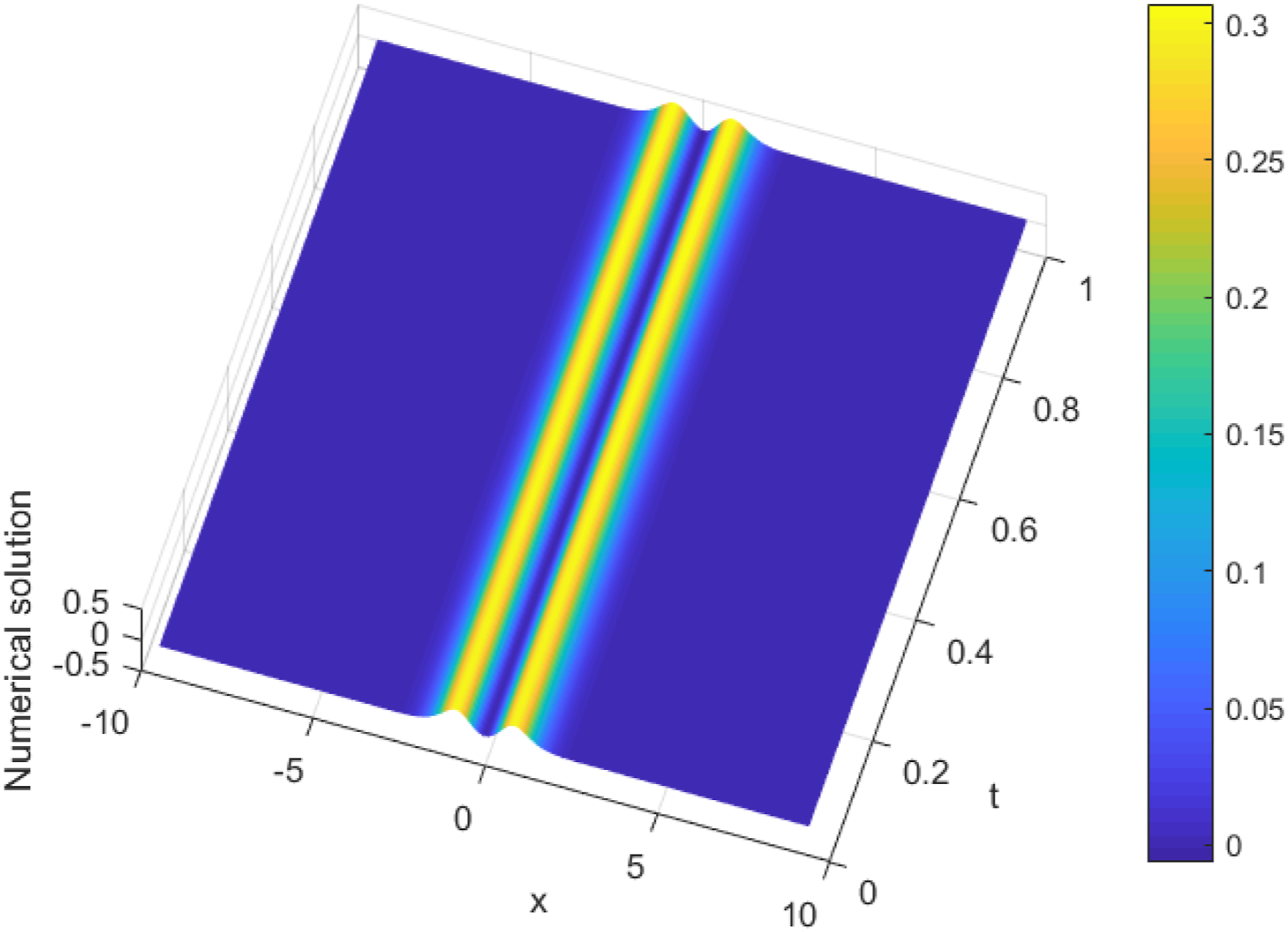
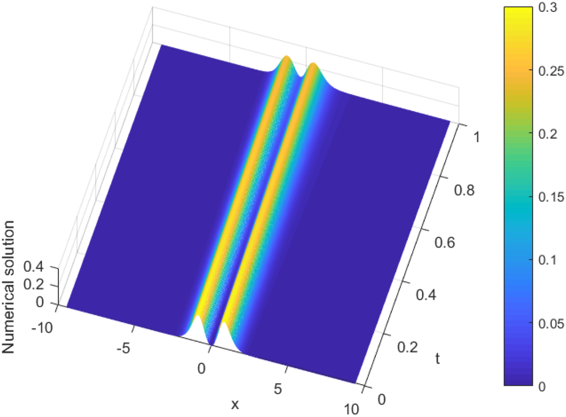
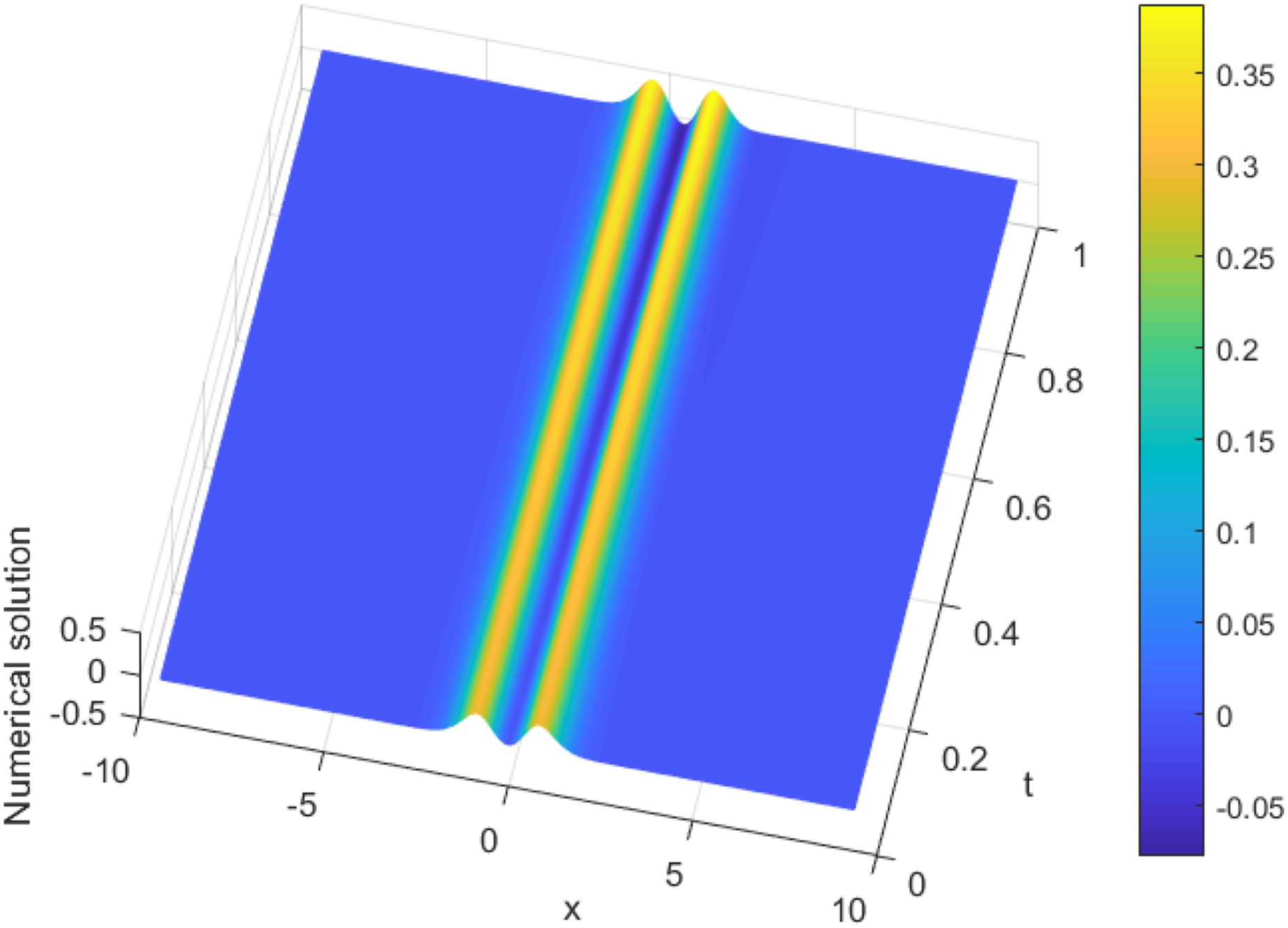
Consider the model (1) with ɛ = 1, α₁ = 1, β = 0, α₂ = 1, α₃ = 0, and α₄ = 1, and the source term f(x, t) is determined by (8) consistent with the chosen solution. The exact solution is as follows

$$u\left(x,t\right)=-\frac{48x\left(t-10\right)+24x^2-12}{{\left(4{\left(t-10\right)}^2+4x\left(t-10\right)+2x^2+1\right)}^2}$$

(8)

The numerical solutions are given in Table 1 and plotted in Figures 1–3. Absolute errors are plotted in Figure 4. Absolute errors at t = 3 are plotted in Figure 5. Absolute errors at x = 8.5 are plotted in Figure 6.

Table 1.

Numerical results at t = 1 for Example 1

x	Exact solution	Numerical solution	Absolute error
−19.125	−0.0011	−0.0011	1.5677 × 10−7
−17.000	−0.0013	−0.0013	7.8469 × 10−7
−14.875	−0.0015	−0.0015	1.9195 × 10−6
−8.5000	−0.0023	−0.0023	2.8552 × 10−6
−2.1250	−0.0018	−0.0018	2.3662 × 10−6
2.1250	0.0037	0.0037	2.3273 × 10−6
8.5000	0.0097	0.0097	1.6182 × 10−6
14.875	0.0014	0.0014	3.1855 × 10−7
17.000	0.0003	0.0003	8.1906 × 10−9
19.125	−0.0002	−0.0002	2.7486 × 10−6

Figure 1.

Numerical solution for Example 1.

Figure 2.

2D-contour plot for Example 1.

Figure 3.

2D-density plot for Example 1.

Figure 4.

Absolute errors for Example 1.

Figure 5.

Absolute errors at t = 3 for Example 1.

Figure 6.

Absolute errors at x = 8.5 for Example 1.

Example 2

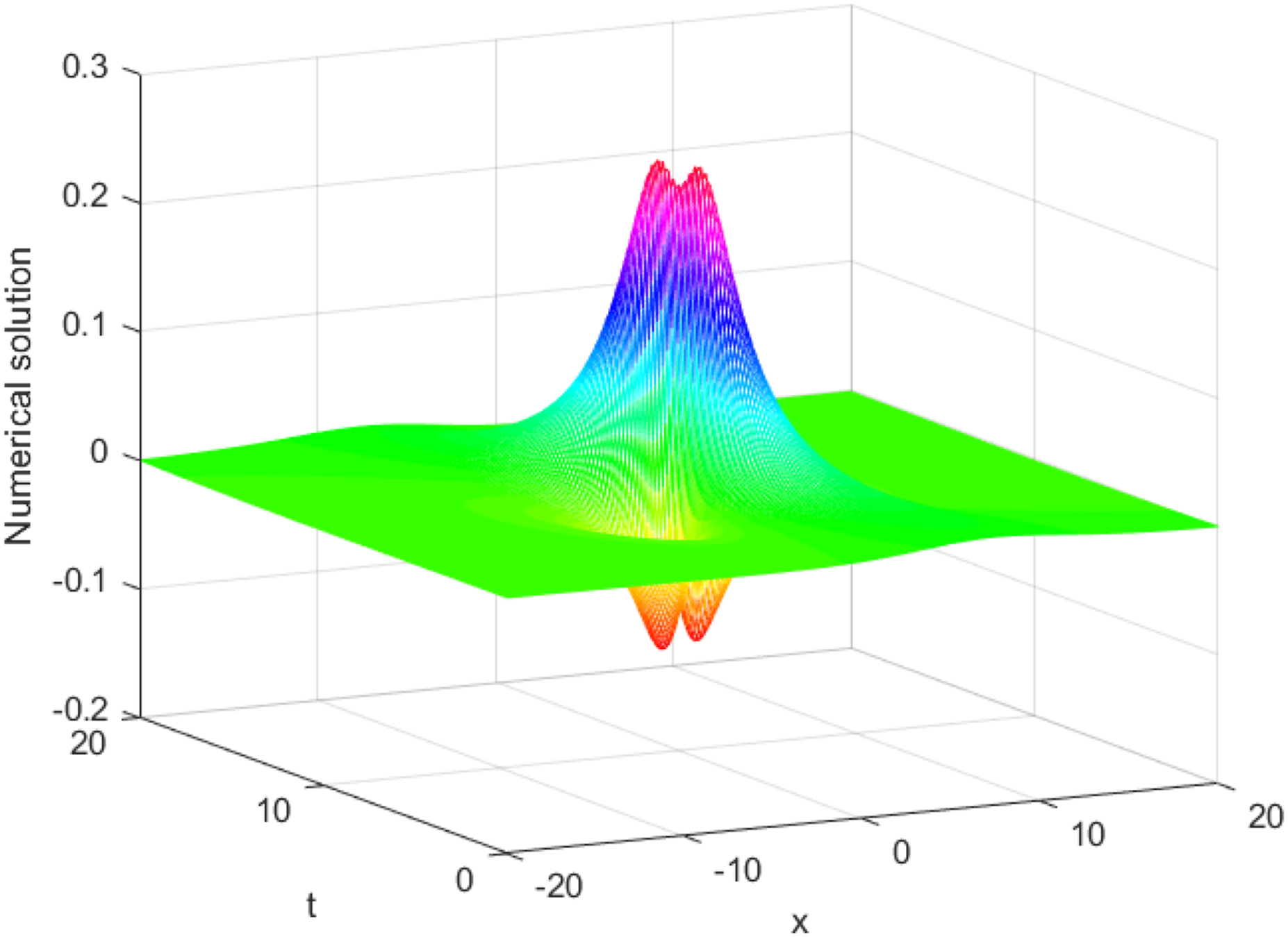
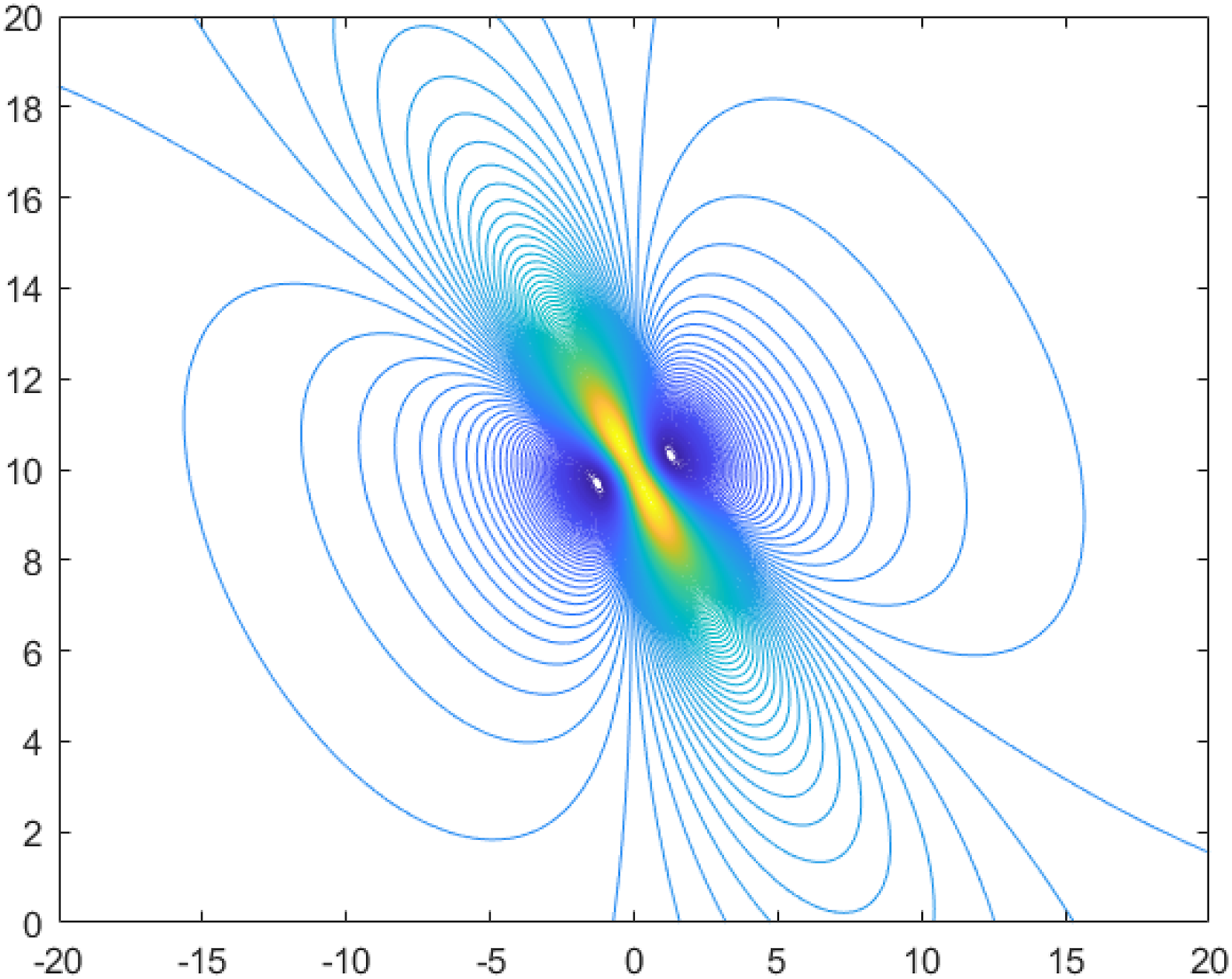
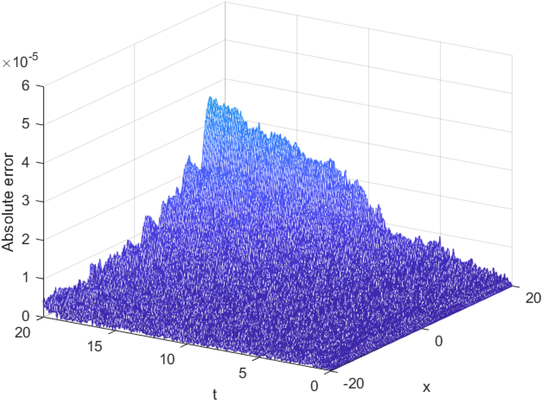
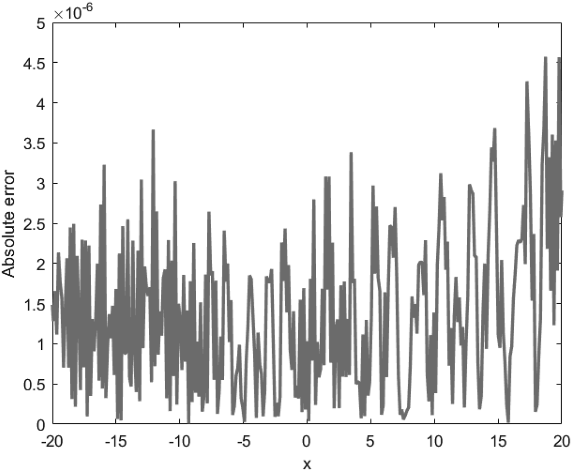
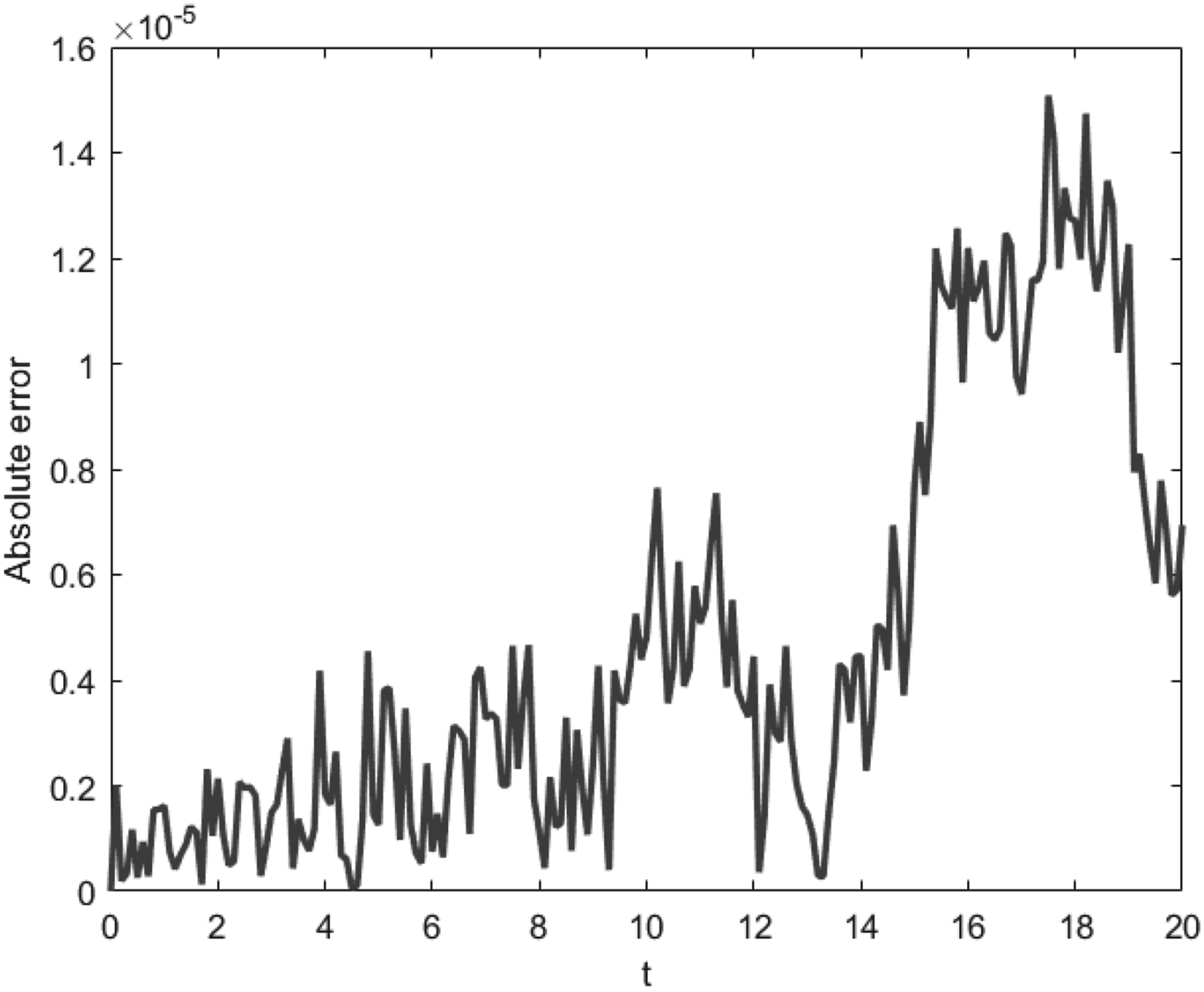
Consider the model (1) with ɛ = 12, α₁ = 0, β = 1, α₂ = 1, α₃ = 1, and α₄ = 1. Referring to the numerical experiment in Aksan’s study,^35,36 the source term f(x, t) is determined by (9) consistent with the chosen solution. The exact solution is as follows

$$u\left(x,t\right)=\mathrm{sech}\left(\frac{3x^2}{50}-t+5\right)$$

(9)

The numerical solutions and analytical solutions are given in Table 2 and plotted in Figures 7 and 8. Absolute errors are plotted in Figure 9. Numerical solutions and analytical solutions at t = 7, 11 are plotted in Figure 10. Absolute errors at t = 1, 10 are plotted in Figure 11. Absolute errors at x = 20 are plotted in Figure 12.

Table 2.

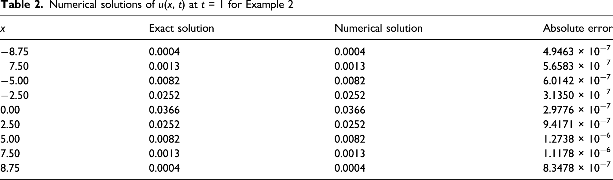
Numerical solutions of u(x, t) at t = 1 for Example 2

x	Exact solution	Numerical solution	Absolute error
−8.75	0.0004	0.0004	4.9463 × 10−7
−7.50	0.0013	0.0013	5.6583 × 10−7
−5.00	0.0082	0.0082	6.0142 × 10−7
−2.50	0.0252	0.0252	3.1350 × 10−7
0.00	0.0366	0.0366	2.9776 × 10−7
2.50	0.0252	0.0252	9.4171 × 10−7
5.00	0.0082	0.0082	1.2738 × 10−6
7.50	0.0013	0.0013	1.1178 × 10−6
8.75	0.0004	0.0004	8.3478 × 10−7

Figure 7.

Numerical solution for Example 2.

Figure 8.

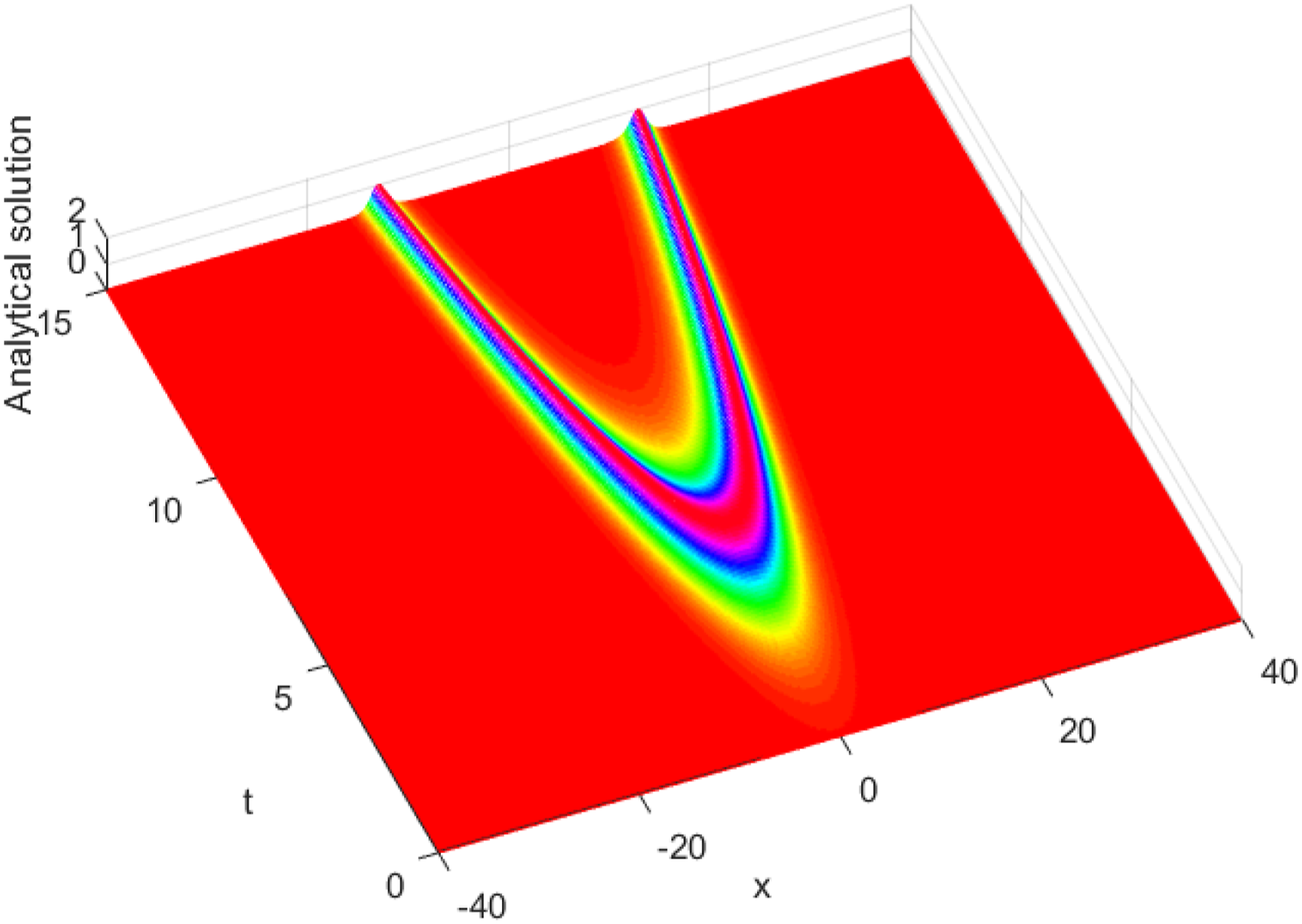
Analytical solution for Example 2.

Figure 9.

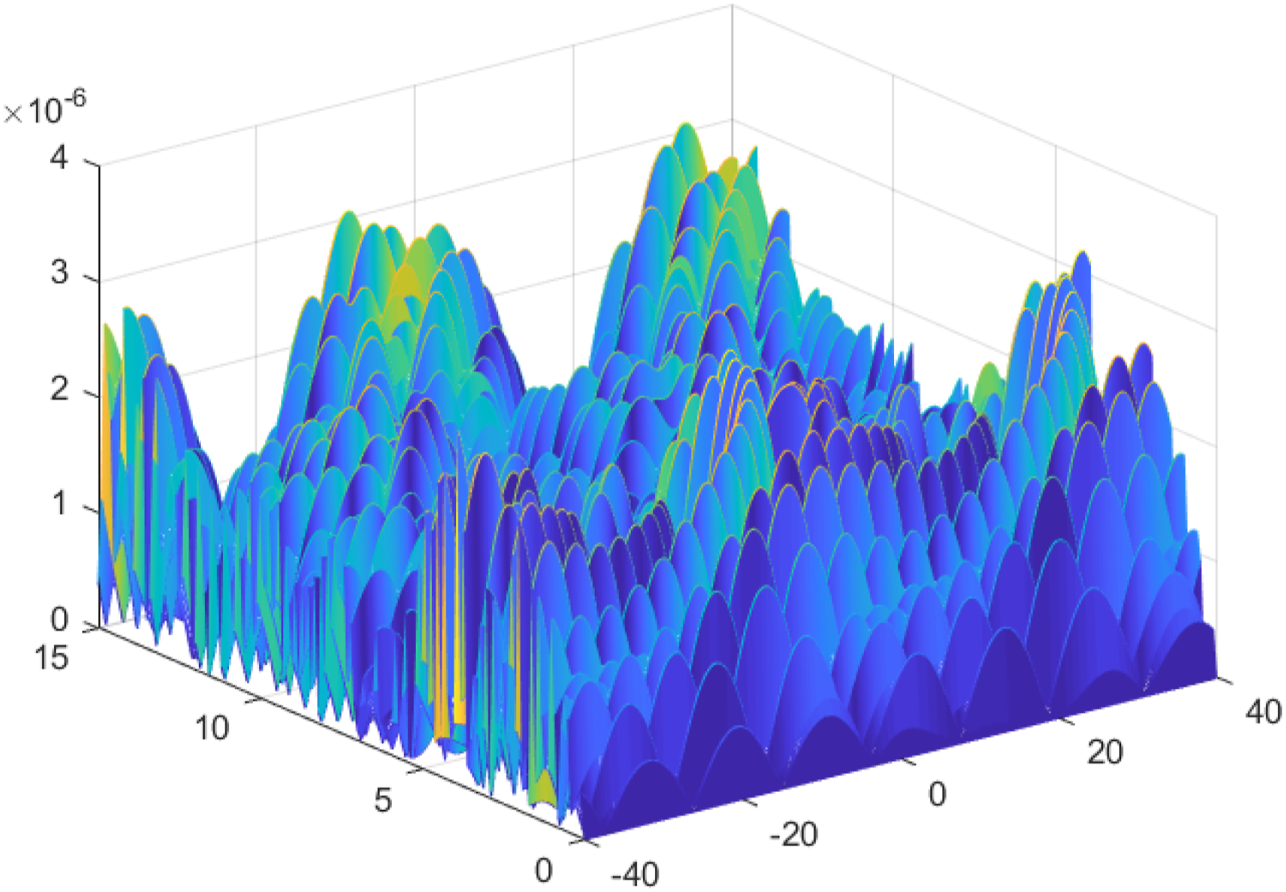
Absolute error for Example 2.

Figure 10.

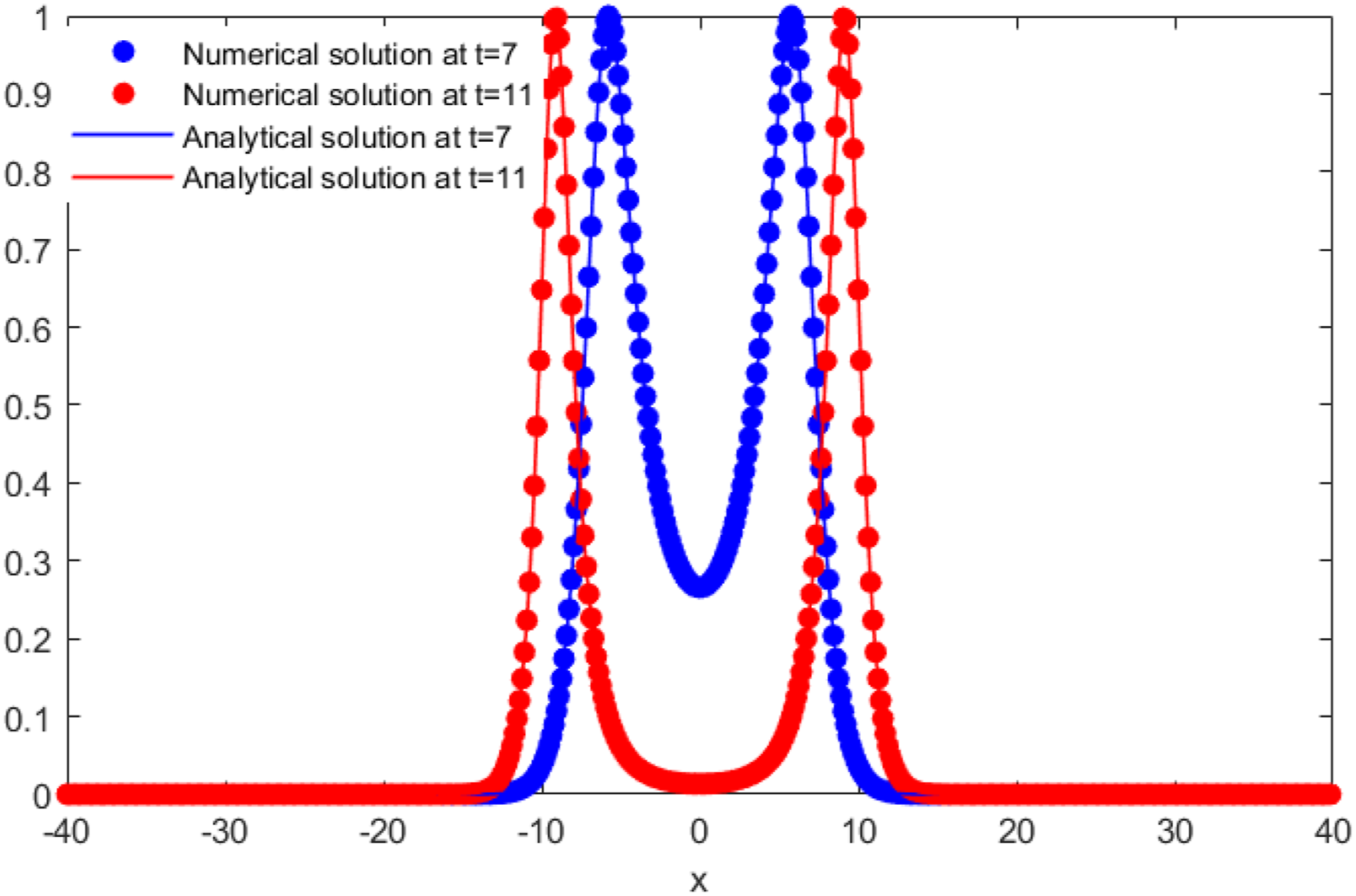
Numerical solution and analytical solution at t = 7, 11 for Example 1.

Figure 11.

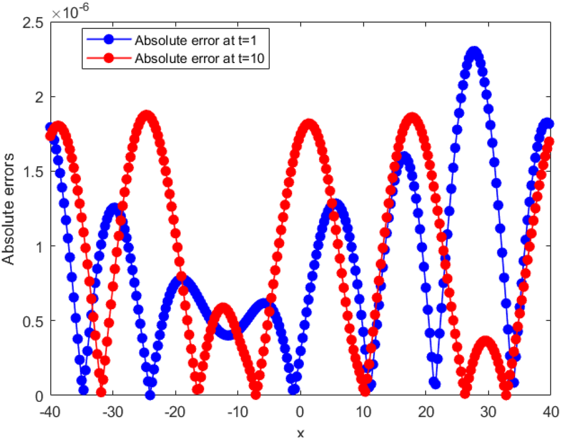
Absolute errors at t = 1, 10 for Example 2.

Figure 12.

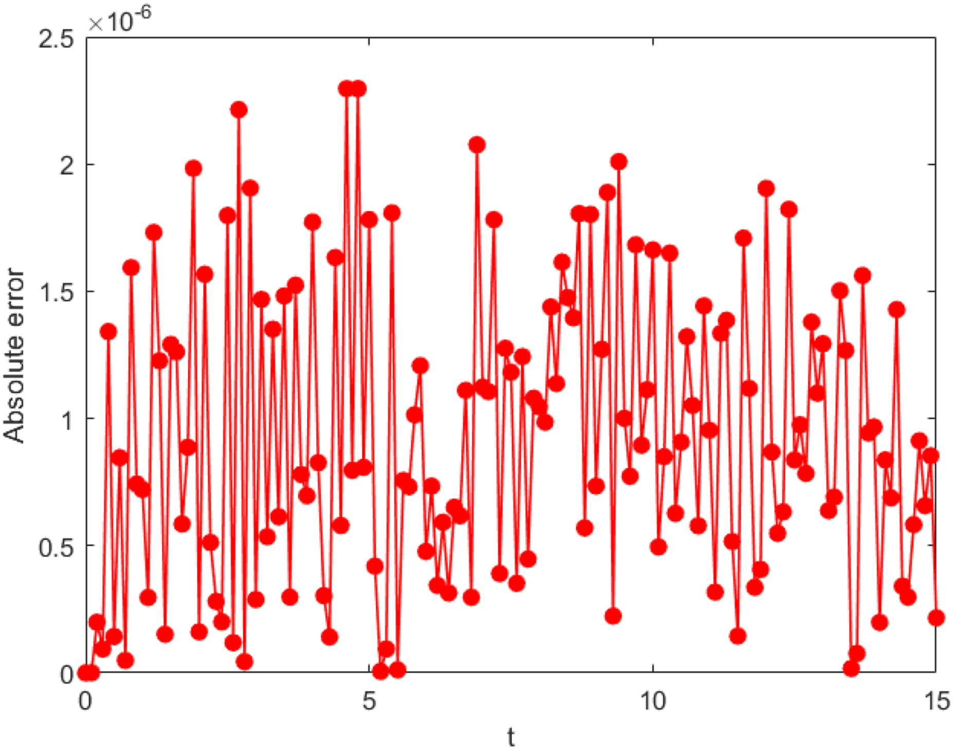
Absolute error at x = 20 for Example 2.

Example 3

Consider the model (1) with ɛ = −1, α₁ = 0, α₂ = 0, and α₄ = 0 which satisfy the initial conditions $u\left(x,0\right)=\tan h\left(x^2\right)e^{-x^2}$ .

By the proposed algorithm, we obtain the numerical solutions which are given in Figures 13–16. Numerical solutions of u(x, t) at α₃ = 1, β = 1/4, 5/6 are plotted in Figures 13 and 14. Numerical solutions at β = 6/5, α₃ = −10, 10 are plotted in Figures 15 and 16.

Figure 13.

Numerical solution at α₃ = 1, β = 1/4 for Example 3.

Figure 14.

Numerical solution at α₃ = 1, β = 6/5 for Example 3.

Figure 15.

Numerical solution at α₃ = −10, β = 6/5 for Example 3.

Figure 16.

Numerical solution at α₃ = 10, β = 6/5 for Example 3.

Example 4

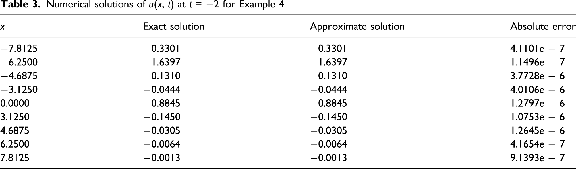
Consider the model (1) with ɛ = −6, α₁ = 0.006, β = 1, α₂ = 0.001, α₃ = t, and α₄ = 0, and the source term f(x, t) is determined by (10) consistent with the chosen solution. The exact solution is as follows

$$u\left(x,t\right)=-\frac{10{\text{e}}^{28x/5}{\text{e}}^t{\text{e}}^{5.0111}-10{\text{e}}^{1583t/125}{\text{e}}^x{\text{e}}^{5.0111}+18{\text{e}}^{729t/125}{\text{e}}^{19x/5}{\text{e}}^{5.0111}-18{\text{e}}^{979t/125}{\text{e}}^{9x/5}{\text{e}}^{5.0111}}{5{\text{e}}^{28x/5}+5{\text{e}}^{1708t/125}{\text{e}}^{5.0111}+5{\text{e}}^{2t}{\text{e}}^{18x/5}{\text{e}}^{5.0111}+10{\text{e}}^{854t/125}{\text{e}}^{14x/5}{\text{e}}^{5.0111}+10{\text{e}}^{854t/125}{\text{e}}^{14x/5}{\text{e}}^{5.0111}+5{\text{e}}^{1458t/125}{\text{e}}^{2x}{\text{e}}^{5.0111}}$$

(10)

Numerical solutions, analytical solutions, and absolute errors are given in Table 3 and Figures 17–20.

Table 3.

Numerical solutions of u(x, t) at t = −2 for Example 4

x	Exact solution	Approximate solution	Absolute error
−7.8125	0.3301	0.3301	4.1101e − 7
−6.2500	1.6397	1.6397	1.1496e − 7
−4.6875	0.1310	0.1310	3.7728e − 6
−3.1250	−0.0444	−0.0444	4.0106e − 6
0.0000	−0.8845	−0.8845	1.2797e − 6
3.1250	−0.1450	−0.1450	1.0753e − 6
4.6875	−0.0305	−0.0305	1.2645e − 6
6.2500	−0.0064	−0.0064	4.1654e − 7
7.8125	−0.0013	−0.0013	9.1393e − 7

Figure 17.

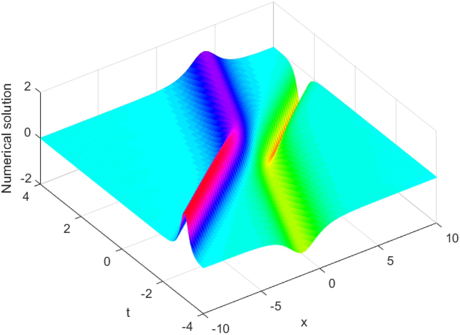
Numerical solution for Example 4.

Figure 18.

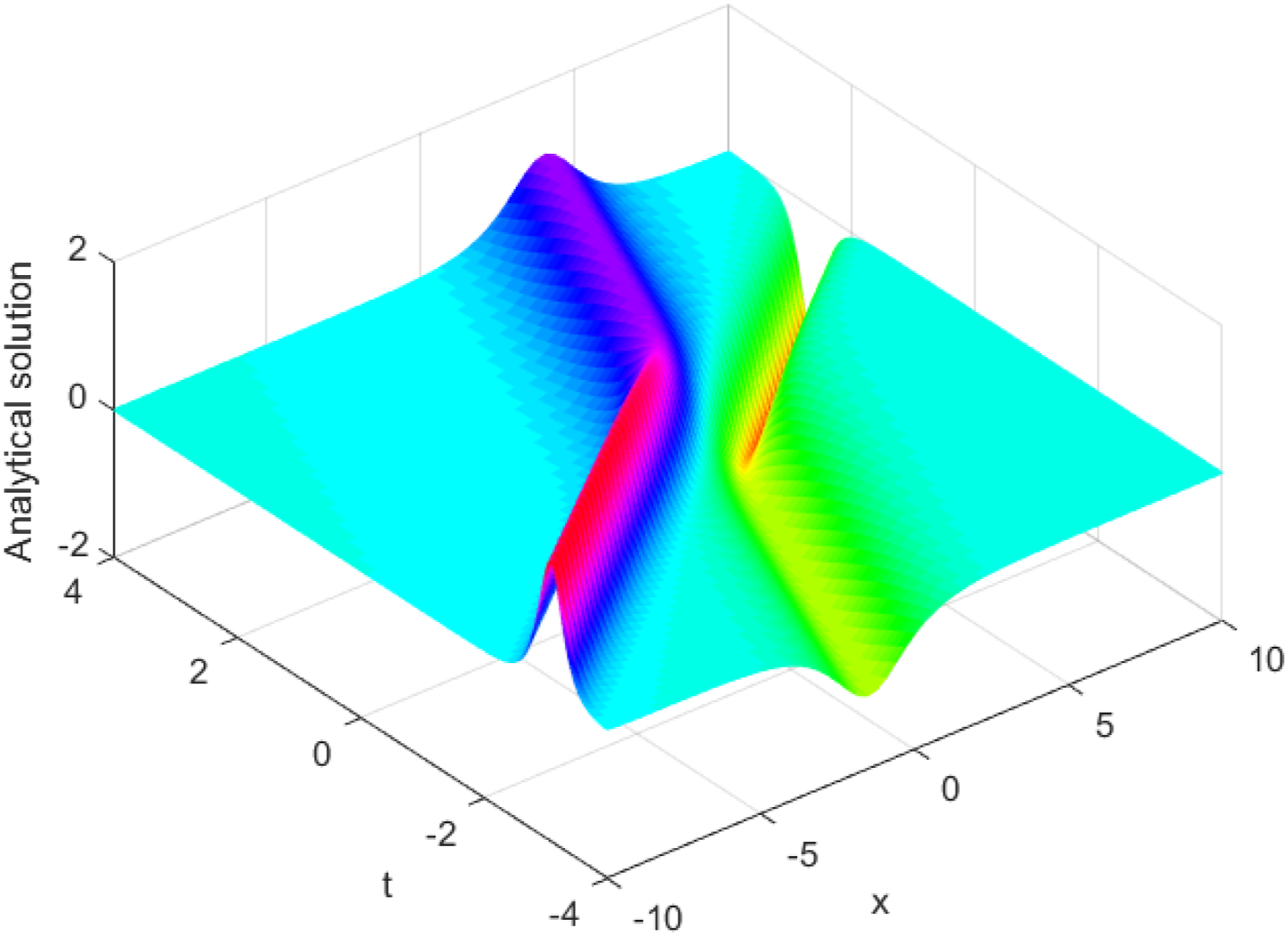
Analytical solution for Example 4.

Figure 19.

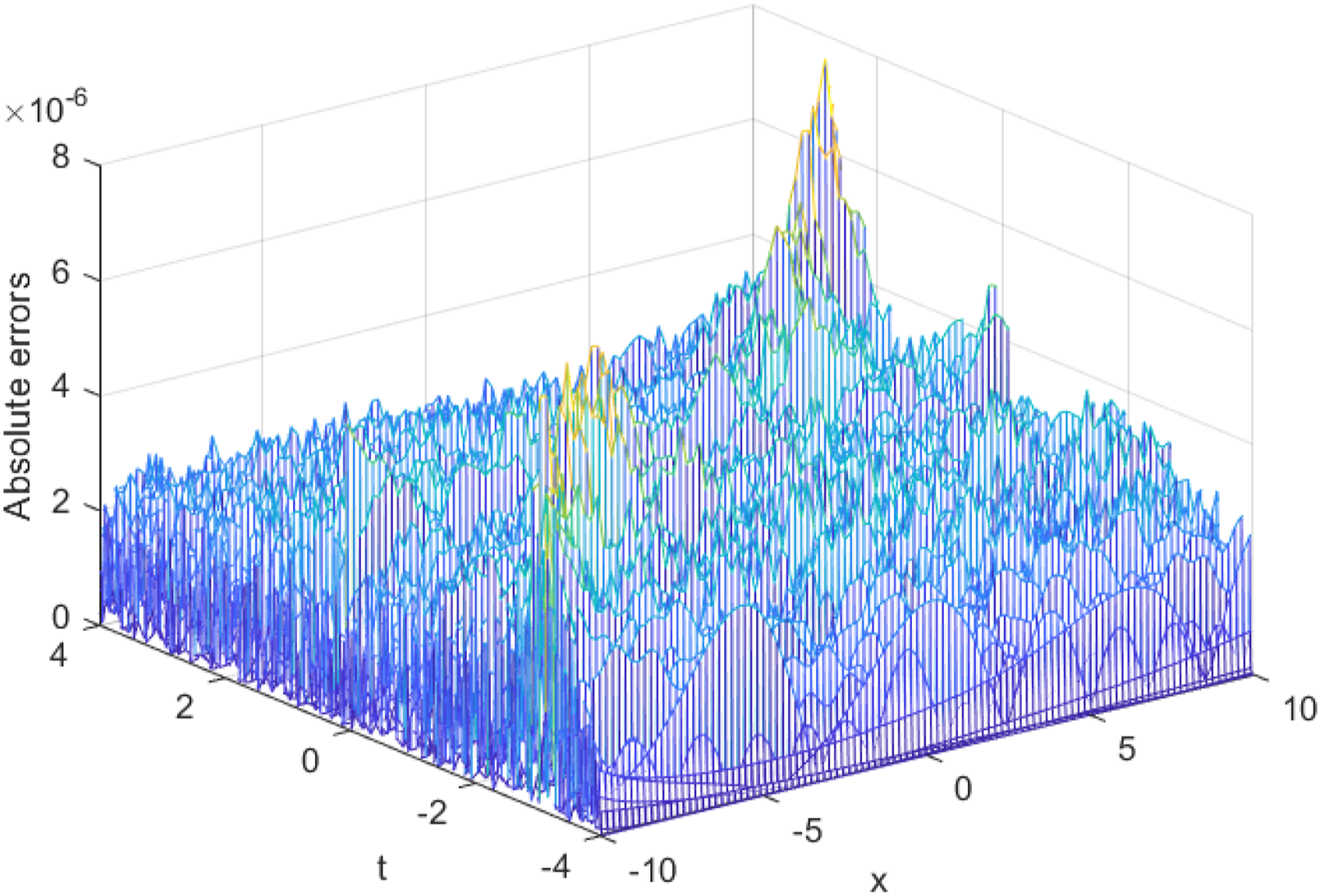
Absolute error for Example 4.

Figure 20.

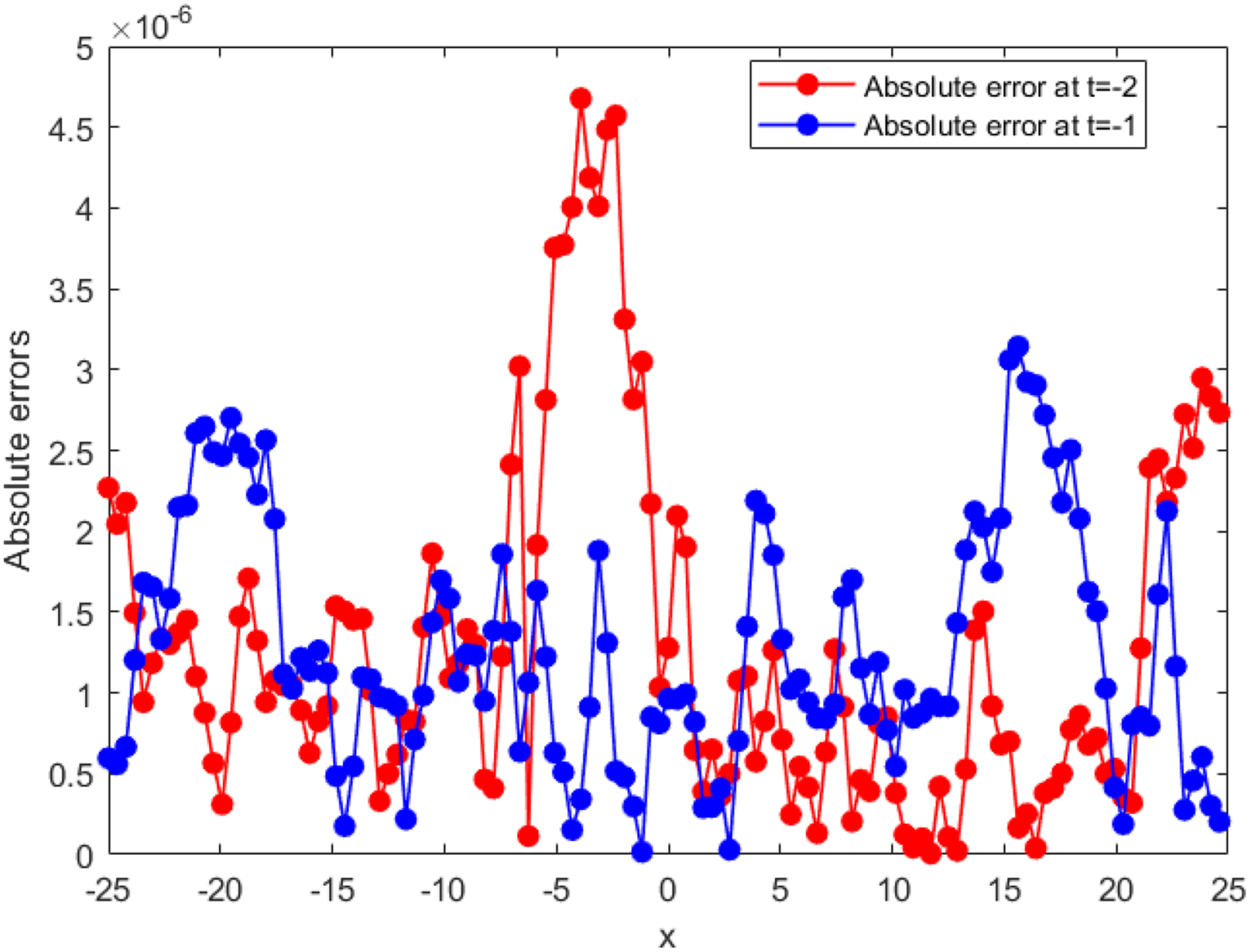
Absolute error at t = −2, −1 for Example 4.

Example 5

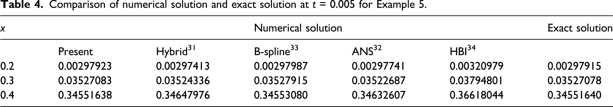
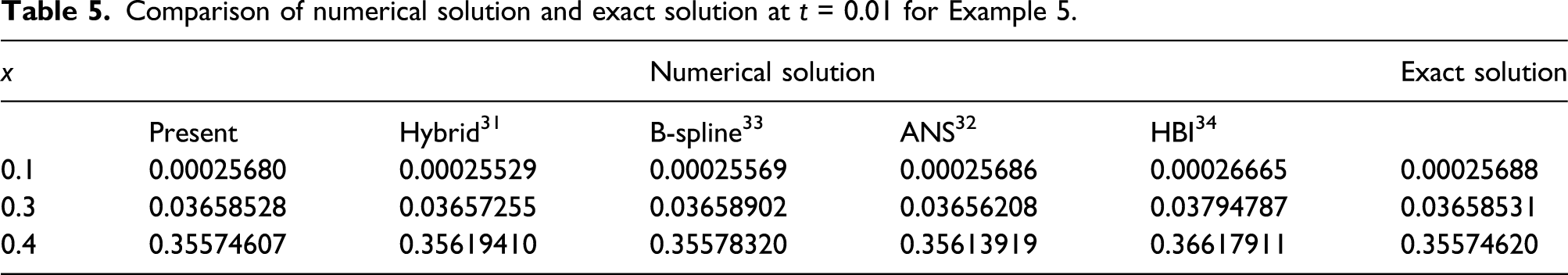
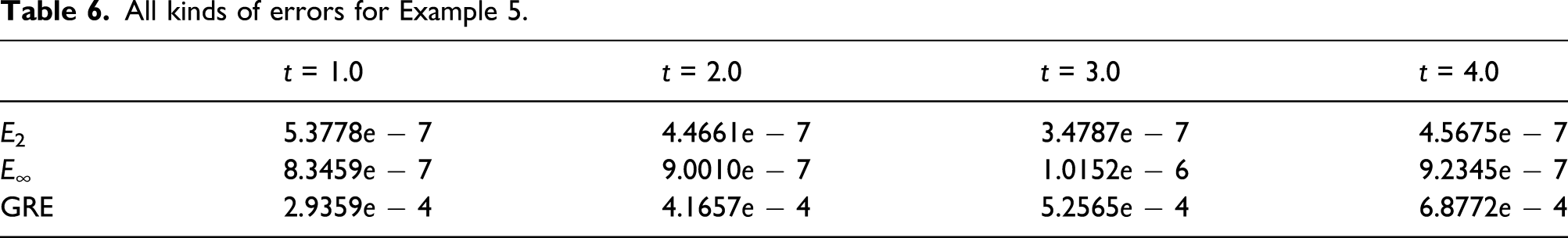
Consider the model (1) with ɛ = 1, α₁ = 0, β = 0, α₂ = 4.84e − 4, and α₃ = α₄ = 0. The exact solution is as follows

$$u\left(x,t\right)=\frac{9}{10\hspace{0.17em}\cos \hspace{0.17em}h{\left(\frac{15\sqrt{30}}{22}t-\frac{25\sqrt{30}}{11}x+6\right)}^2}$$

(11)

By the present method, we obtain the numerical results which are given Tables 4–6. In Tables 4 and 5, we show the numerical solutions by the present method, hybrid numerical method, Galerkin B-spline finite element method, ANS, HBI, and the exact values at the selected notes for t = 0.005, 0.01.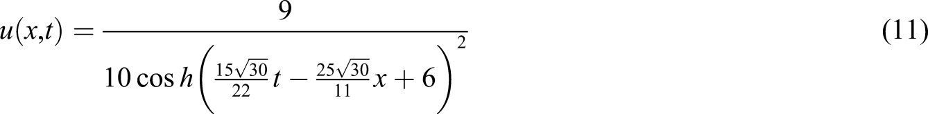

Table 4.

Comparison of numerical solution and exact solution at t = 0.005 for Example 5.

x			Numerical solution			Exact solution
	Present	Hybrid 31	B-spline 33	ANS 32	HBI 34
0.2	0.00297923	0.00297413	0.00297987	0.00297741	0.00320979	0.00297915
0.3	0.03527083	0.03524336	0.03527915	0.03522687	0.03794801	0.03527078
0.4	0.34551638	0.34647976	0.34553080	0.34632607	0.36618044	0.34551640

Table 5.

Comparison of numerical solution and exact solution at t = 0.01 for Example 5.

x			Numerical solution			Exact solution
	Present	Hybrid 31	B-spline 33	ANS 32	HBI 34
0.1	0.00025680	0.00025529	0.00025569	0.00025686	0.00026665	0.00025688
0.3	0.03658528	0.03657255	0.03658902	0.03656208	0.03794787	0.03658531
0.4	0.35574607	0.35619410	0.35578320	0.35613919	0.36617911	0.35574620

Table 6.

All kinds of errors for Example 5.

	t = 1.0	t = 2.0	t = 3.0	t = 4.0
E 2	5.3778e − 7	4.4661e − 7	3.4787e − 7	4.5675e − 7
E ∞	8.3459e − 7	9.0010e − 7	1.0152e − 6	9.2345e − 7
GRE	2.9359e − 4	4.1657e − 4	5.2565e − 4	6.8772e − 4

Conclusions and remarks

In the article, we propose a Fourier spectral Runge–Kutta method for a class of space fractional nonlinear vibration equation. A numerical method that combines the Fourier spectral method with the Runge–Kutta method is proposed to study a class of space fractional nonlinear vibration equation with periodic boundary condition. The accuracy and efficiency of the proposed method have been demonstrated by the numerical results. This approach has general meanings and thus can be used to solve many same types of nonlinear space fractional partial differential equations in science and engineering. Comparisons of the obtained solutions and numerical results show that this method is effective and convenient. Some new numerical results are shown by using this new approach, and the results have a good agreement with theoretical results.