Sage Journals: Discover world-class research

Abstract

This paper presents a bio-evolutionary metaheuristic approach to study the harmonically oscillating behavior of the Duffing equation. The proposed methodology is an amalgamation of the artificial neural network with the firefly algorithm. A novelty in the activation of neurons of artificial neural network is described using the cosine function with the angular frequency. Chronologically, artificial neural network approximates discretizes the nonlinear functions of the governing problem, which then undergoes an optimization process by the firefly algorithm that then later generates the effective values of the unknown parameters. Generally, the algorithm and implementation of the scheme are assimilated by considering an application of Duffing-harmonic oscillator. Some error measurements, in order to discuss the convergence and accuracy of the scheme, are also visualized through tables and graphs. An effective optimized relationship between the angular frequency and amplitude is derived and its results are depicted in a tabular form. The comparison of the proposed methodology is also deliberated by homotopy perturbation method. Moreover, the geometrical illustration of the trajectories of the dynamic system is also added in the phase plane for different values of amplitude and angular frequency.

Keywords

Nonlinear oscillator optimization amplitude–frequency relation

Introduction

Problems of nonlinear vibration in conservative systems, bearing a wide history, have been interpreted to a great extent, in order to study various parametric behaviors of nonlinear vibrations of several mechanical objects.^1–3 In this regard, several methods have been established to analyze these problems, analytically as well as numerically.^4–6 Particularly, among many well-known oscillatory equations, the Duffing equation is found to be the most widely studied equation for its eminent applications in different fields of science, engineering, and biology. He et al.⁷ discussed Duffing-harmonic equation and established a relationship of between the frequency and amplitude of the oscillations using the Hamiltonian approach. Considering the same method, He et al. also discussed the approximate frequency–amplitude relationship of the nonlinear oscillators.⁸ Further, Ren⁹ restudied and derived the He's frequency–amplitude formulation for nonlinear oscillators from an ancient Chinese mathematical algorithm. Succinctly, the oscillating and chaotic nature of this nonlinear model has augmented a miraculous notion in the literature, as it imitates the dynamics of our natural world.^10–16

In essence, the following equation for Duffing-harmonic oscillation is formulated and studied, i.e.

Y ″ (t) + \frac{Y^{3} (t)}{1 + Y^{2} (t)} = 0, Y (0) = A, Y' (0) = 0

(1)

where

A

represents the amplitude of the oscillation. The key objective of the paper is to establish a technique that provides effective solutions for the wide range of

A

. Accordingly, the aim is achieved by using the technique based on artificial neural network (ANN)^17–20 and the firefly optimization algorithm.^21,22 The accuracy of the algorithm depends on the value of adjustable parameters, i.e. the weights of the ANNs. Therefore, to gain accurate approximations of these parameters, the training of these weights is made by a global optimizer firefly algorithm (FFA). For the governing oscillator (1), a novel activation function for neurons of ANN is ascertained by means of a cosine function with the angular frequency. In addition, the accuracy, convergence, and effectiveness of the established scheme are determined out by the comparison plots of the attained outcomes with the exact solutions together with the values of mean absolute error and root mean square error.

The remaining structure of the paper is defined as follows: the next section delineates the utilization of the proposed methodology on Duffing-harmonic oscillation in detail with the addition of the flowchart of the scheme and an error bound relation. Then, the acquired relations of frequency and amplitude with the efficacious discussion on the behavior of oscillation and weights of the neural network are discussed. The final section covers the concluding remarks and motivational recommendations for the future work.

Methodological configuration

In this section, the implementation of the ANN on Duffing-harmonic oscillation is elaborated as follows.

Intelligent approximation

Any arbitrary continuous function and its derivatives on a compact set can be approximated by taking into account the components of feed forward artificial neural, i.e. multiple inputs, single hidden layer with a linear output layer without bias. The solution $Y$ of equation (1) can be approximated by the following continuous mapping¹⁸

\hat{Y} (t, γ) = \sum_{i = 1}^{N} γ_{i} f (z)

(2)

where

γ_{i}

are real-valued unknown weights of the network,

N

is the number of neurons,

f

is said to be the activation function and

z

is said to be a linear sum defined as,

z = (2 i - 1) ω t

. For the case of nonlinear oscillation,^7,8 the trial solution of

Y

is accomplished by taking

f (z) = \cos (z)

in the activation function

f

. Therefore, the weighted sum of second-order derivative

Y^{″}

, would become

{\hat{Y}}^{″} (t, γ) = \sum_{i = 1}^{N} γ_{i} ω^{2} {(2 i - 1)}^{2} f^{″} (z)

(3)

The estimated model for equation (1) can be formulated by substituting the weighted sums of the networks, equations (2) and (3), in equation (1). It is well known that the angular frequency $ω$ in the Duffing-harmonic oscillation depends on the amplitude of motion $A$ . Taking into account different assumptions for $ω$ , some techniques have been illustrated that provide accurate results but for small values of $A$ . These techniques have illustrated that the error for the angular frequency could be up to 1.60% for the range $0.01 < A < 100$ .¹⁰ Apparently, it is difficult to obtain a method, which has the capability to give an accurate result with the error less than 1.60% in a wide range of $A$ . Hence, keeping this in mind, a highly effective numerical procedure of optimization is proposed that produces accurate results and produces the least errors.

Fitness function

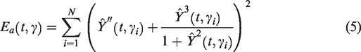
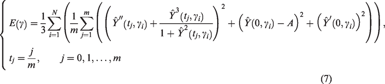
The robustness of any methodology is examined by defining an error function, which is formed by substituting the approximated functions $\hat{Y} (t, γ)$ and ${\hat{Y}}^{″} (t, γ)$ in equation (1). The objective function for the optimization algorithm is to minimize the mean square error, outlined as follows

E (γ) = \frac{1}{3} (E_{a} (t, γ) + E_{c 1} (γ) + E_{c 2} (γ))

(4)

where

E_{a} (t, γ)

is constructed as

E_{a} (t, γ) = \sum_{i = 1}^{N} {({\hat{Y}}^{″} (t, γ_{i}) + \frac{{\hat{Y}}^{3} (t, γ_{i})}{1 + {\hat{Y}}^{2} (t, γ_{i})})}^{2}

(5)

and

E_{c 1} (γ)

E_{c 2} (γ)

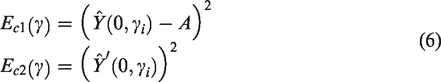
are expanded by using the initial conditions of equation (1) as

\begin{array}{l} E_{c 1} (γ) = {(\hat{Y} (0, γ_{i}) - A)}^{2} \\ E_{c 2} (γ) = {({\hat{Y}}^{'} (0, γ_{i}))}^{2} \end{array}

(6)

On discretizing $t \in [0, 1]$ , for $m$ equal segments in equation (5), the fitness function of equation (4) takes the following form

{\begin{cases} E (γ) = \frac{1}{3} \sum_{i = 1}^{N} (\frac{1}{m} \sum_{j = 1}^{m} ({({\hat{Y}}^{″} (t_{j}, γ_{i}) + \frac{{\hat{Y}}^{3} (t_{j}, γ_{i})}{1 + {\hat{Y}}^{2} (t_{j}, γ_{i})})}^{2} + {(\hat{Y} (0, γ_{i}) - A)}^{2} + {({\hat{Y}}^{'} (0, γ_{i}))}^{2})), \\ t_{j} = \frac{j}{m}, j = 0, 1, \dots, m \end{cases}

(7)

As evident, the adjustable parameters $γ_{i}$ used in equations (2) and (3), for which $E_{c 1}$ , $E_{c 2}$ and $E_{a} (γ)$ come closer to zero, the value of $E$ also approaches 0, which then produces approximate solution, $\hat{Y} (t)$ that are highly compatible with the exact solution.

FFA

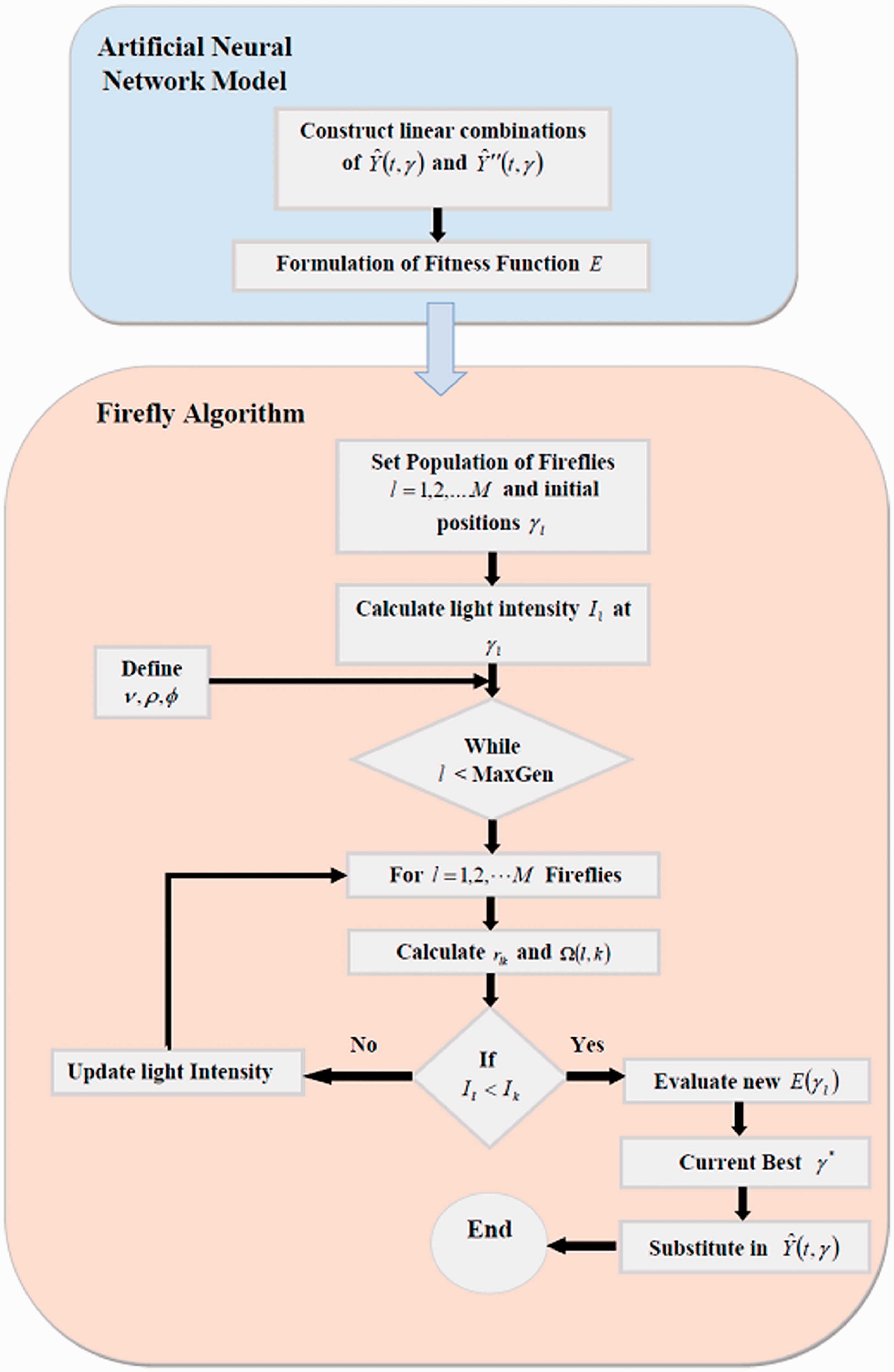
Nowadays, metaheuristic optimization algorithms are playing an important role for being very promising in solving optimization problems.²³ Most of these algorithms are structured in such a way that their systematic procedures meticulously work like biological creatures. Here, we consider the FFA, for the optimization purpose of the fitness function and obtain precise solutions of weights of ANN. Being a nature-inspired algorithm, the system of FFA methodically functions like the biotic behavior of the fireflies.^21,22 The algorithm is carried out as follows:

Let, $B_{M \times N}$ represent firefly swarm, where $N$ is the number of neurons (weights) to be minimized and $M$ are the number of fireflies, where the associated position of firefly $l$ is $γ_{l} \in ℜ^{ℵ}, l = 1, 2, \dots, M$ .

The light intensity used by fireflies to attract one another is denoted by $I$ , which inversely depends on the distance between the species and air absorption of light.

The error function $E (γ_{l})$ is considered as the objective function, to convert the governing problem into an optimization problem. On the other hand, it is used to measure the brightness at a particular position.

Fireflies move randomly so the distance $r_{l k}$ varies between firefly $l$ and firefly $k$ . The strength of attractiveness $Ω$ of a firefly, which is directly proportional to the light intensity of the adjacent firefly, is outlined as

Ω (l, k) = σ_{0} e^{- λ r_{l k}^{2}}

(8)

where $σ_{0}$ is the initial attractiveness and $λ$ is the light absorption coefficient.

Consequently, if the light intensity of a firefly at the position $γ_{l}$ is brighter than that at $γ_{k}$ , then the movement of firefly $l$ towards firefly $k$ is computed as

γ_{k}^{q + 1} = γ_{k}^{q} + Ω (l, k) (γ^{q}_{l} - γ^{q}_{k}) + ρ (ν \frac{1}{2})

(9)

where $ρ$ is a randomization factor that controls the magnitude of the stochastic perturbation of $γ_{k}^{q}$ , and $ν \in (0, 1)$ is random number generator.

When all the fireflies have been modified, the best firefly $ψ^{*}$ will perform a controlled random walk across the search space

γ^{*} = γ_{l}^{*} + ρ (ϕ \frac{1}{2}), ϕ \neq ν, ϕ \in (0, 1)

(10)

Suppose, $γ^{*}$ is the optimal solution of the optimization problem (8), then by substituting it into equation (2), the approximate solution of equation (1) is achieved efficiently. The flowchart of the proposed algorithm is also demonstrated graphically in Figure 1.

Figure 1.

The procedural layout of the proposed scheme.

Error bounds and convergence

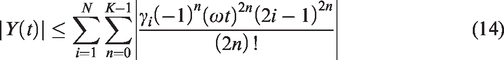
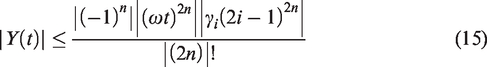
In this sequel, an assessment for the accuracy and boundedness of the solutions of $\hat{Y} (t)$ is carried out. Since the continuous mapping expansion (2) is contemplated as the approximate solution of equation (1), it must satisfy the following error function, i.e. for $t = t_{j} \in [0, 1], j = 0, 1, 2, \dots m$

E F_{N} (t_{j}) = | Y^{*} (t_{j}) - {\hat{Y}}_{t r i a l} (t_{j}) | ≅ 0

(11)

where

Y^{*} (t_{j})

is the exact solution of the governing problem (1) at different values of

t_{j} \in [0, 1]

. Correspondingly, if

E F_{N} (t_{j}) \leq 10^{- μ}

with

μ

be any positive integer, then the truncation limit

N

is enlarged until

E F_{N} (t_{j})

, at each point becomes diminutive than the specified value

10^{- μ}

Let $Y (t)$ is a square integrable continuous function in interval $[0, 1]$ , so that the series (2) becomes convergent for $Y (t)$ . Thus, equation (2) can be expanded as

Y (t) = \sum_{i = 1}^{N} \sum_{n = 0}^{\infty} \frac{γ_{i} {(- 1)}^{n} {(ω t)}^{2 n} {(2 i - 1)}^{2 n}}{(2 n)!}

(12)

Since $Y (t)$ is bounded $\forall n \in N$ , we can write

| Y (t) | \leq | \sum_{i = 1}^{N} \sum_{n = 0}^{K - 1} \frac{γ_{i} {(- 1)}^{n} {(ω t)}^{2 n} {(2 i - 1)}^{2 n}}{(2 n)!} | + R_{K}

(13)

Here, $R_{K} = | \lim_{K \to \infty} \sum_{i = 1}^{N} \frac{γ_{i} {(- 1)}^{K} {(ω t)}^{2 K} {(2 i - 1)}^{2 K}}{(2 K)!} |$ , as $K \to \infty$ , $R_{K} \to 0$ . The association of summation gives

| Y (t) | \leq \sum_{i = 1}^{N} \sum_{n = 0}^{K - 1} | \frac{γ_{i} {(- 1)}^{n} {(ω t)}^{2 n} {(2 i - 1)}^{2 n}}{(2 n)!} |

(14)

Using multiplicative property, we get

| Y (t) | \leq \frac{| {(- 1)}^{n} | | {(ω t)}^{2 n} | | γ_{i} {(2 i - 1)}^{2 n} |}{| (2 n) |!}

(15)

Since $Y (t)$ is bounded, then $\frac{{(- 1)}^{n}}{(2 n)!}$ , ${(ω t)}^{n}$ and ${(2 i - 1)}^{2 n}$ are also bounded; therefore, there exist numbers $W, H, K > 0$ , such that $| \frac{{(- 1)}^{n}}{(2 n)!} | < \frac{1}{H}$ , $| {(ω t)}^{2 n} | < W$ and $| {(2 i - 1)}^{2 n} | < K$ , $\forall n \in N$ . Hence

| Y (t) | < \frac{W K}{H}

(16)

where it can be perceptibly observed that the error bound is inversely proportional to the number of neurons. Hence, the series expansion (2) converges to the exact solution of equation (1), as number of neurons approaches infinity, i.e.

n \to \infty

Frequency–amplitude relationship

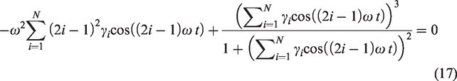
The proposed method can be advantageously used to acquire optimized association between angular frequency and amplitude of Duffing-harmonic oscillation. After substituting the weighted sums, i.e. equations (2) to (3) in equation (1), we get

- ω^{2} \sum_{i = 1}^{N} {(2 i - 1)}^{2} γ_{i} \cos ((2 i - 1) ω t) + \frac{{(\sum_{i = 1}^{N} γ_{i} \cos ((2 i - 1) ω t))}^{3}}{1 + {(\sum_{i = 1}^{N} γ_{i} \cos ((2 i - 1) ω t))}^{2}} = 0

(17)

Considering the acceleration at the time $t = 0$ and using equation (1), in equation (2), we attain

- ω^{2} \sum_{i = 1}^{N} {(2 i - 1)}^{2} γ_{i} + \frac{A^{3}}{1 + A^{2}} = 0

(18)

Therefore, we obtain the following relationship by taking $β_{i} = \sum_{i = 1}^{N} {(2 i - 1)}^{2} γ_{i}$

ω = \frac{A^{3 / 2}}{\sqrt{(1 + A^{2}) β_{i}}}

(19)

Homotopy perturbation method

The parameter-expansion methods are widely used in dealing with nonlinear problems. In this section, the implementation of homotopy perturbation method (HPM)¹⁶ is shown, which will be exercised for the comparative study of the proposed technique in results discussion. The construction of homotopy equation (1) is carried out as

Y ″ (t) + (- 1) Y + p ((Y ″ Y^{2}) + Y + Y^{3}) = 0

(20)

On expanding the coefficient of the linear term (−1) and the solution into the following forms²³

- 1 = ω^{2} + θ_{1} p + θ_{2} p^{2} + \dots

(21)

Y = Y_{0} + Y_{1} p + Y_{2} p^{2} + \dots

(22)

Submitting equations (22) and (23) into equation (21), and processing the perturbation method, we obtain the following linear equations

Y_{0} ″ (t) + ω^{2} Y_{0} = 0, Y_{0} (0) = A, Y_{0}' (0) = 0

(23)

Y_{1} ″ + ω^{2} Y_{1} + θ_{1} Y_{0} + Y_{0} ″ Y_{0}^{2} + Y_{0} + Y_{0} 3 = 0, Y_{0} (0) = A, Y_{0}' (0) = 0

(24)

Calculating $Y_{0}$ from equation (23) we get

Y_{0} = A \cos (ω t)

(25)

Substituting equation (25) into equation (24) and on further simplification we attain

Y_{1} ″ + ω^{2} Y_{1} + (θ_{1} A + A + \frac{3}{4} (A^{3} - A^{3} ω^{2})) \cos (ω t) + \frac{3}{4} (A^{3} - A^{3} ω^{2}) \cos (3 ω t) = 0

(26)

No secular term in $Y_{1}$ requires that

θ_{1} A + A + \frac{3}{4} A^{3} (1 - ω^{2}) = 0

(27)

If the first order approximate is searched, then from equation (21), we have $θ_{1} + ω^{2} = - 1$ . Thus, from equation (29) the following frequency can be generated

ω = \sqrt{\frac{(3 / 4) A^{2}}{(1 + (3 / 4) A^{2})}}

(28)

Equation (28) is valid for the case when $A > 0$ , because when $A < 0$ , there does not exist any periodic solution to equation (1).

Simulation and results

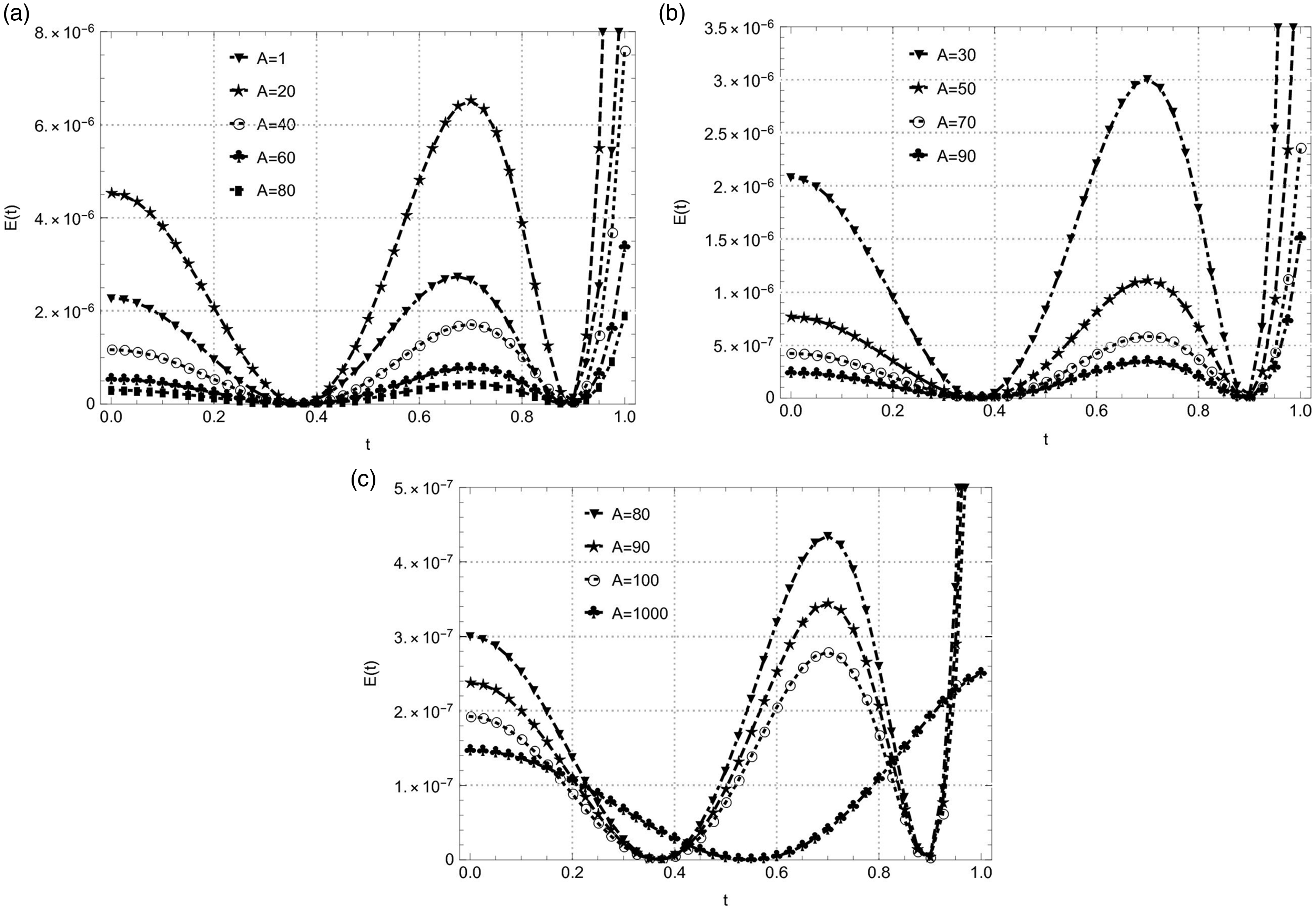
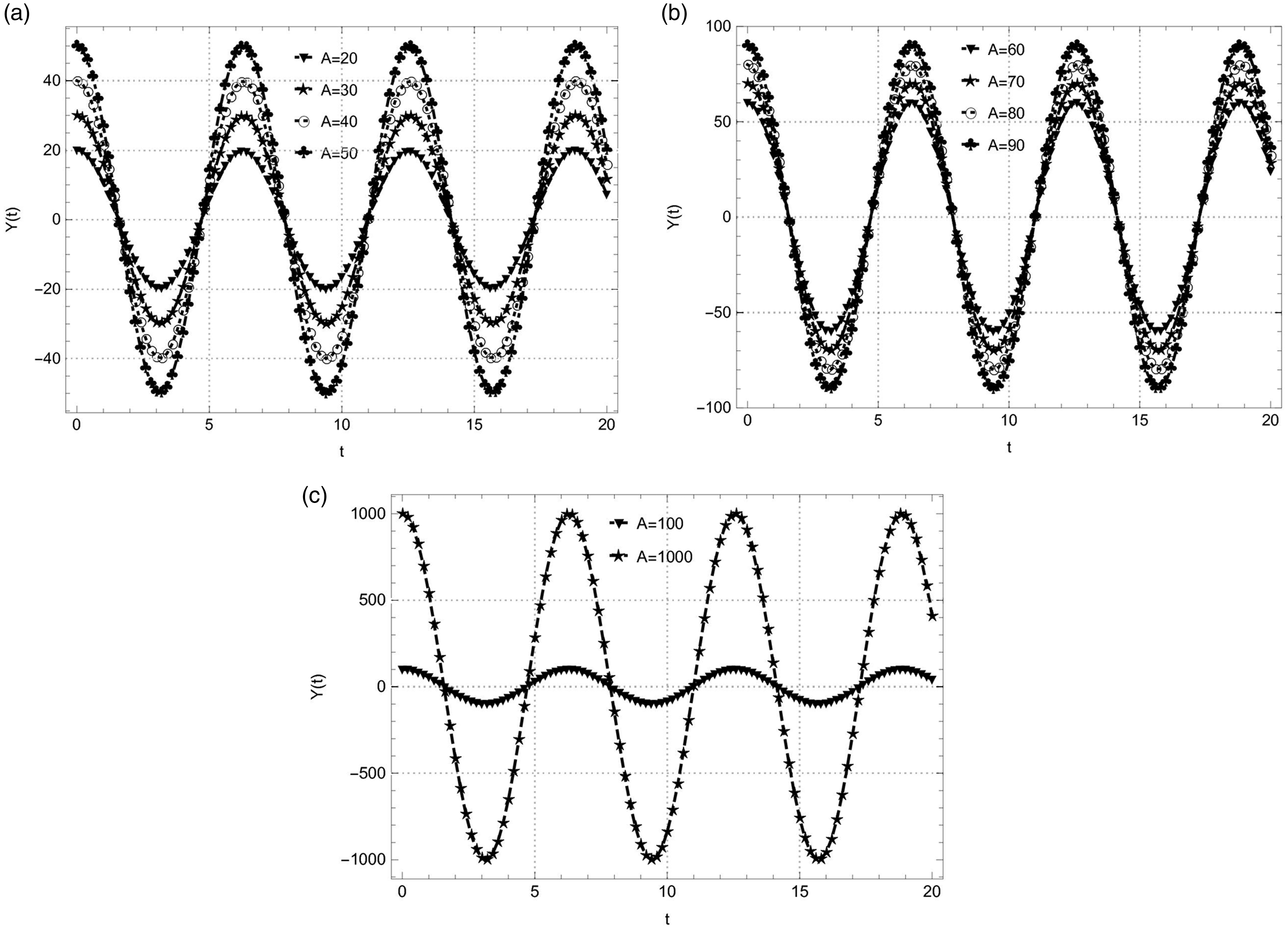
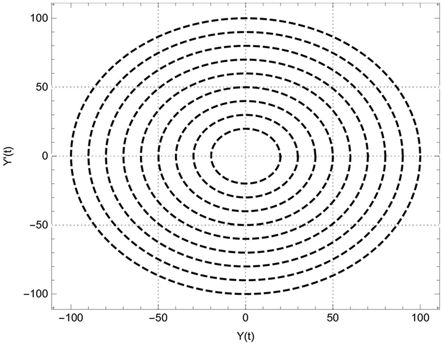
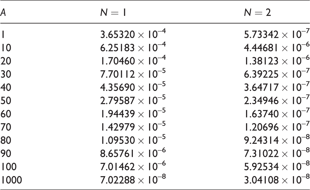
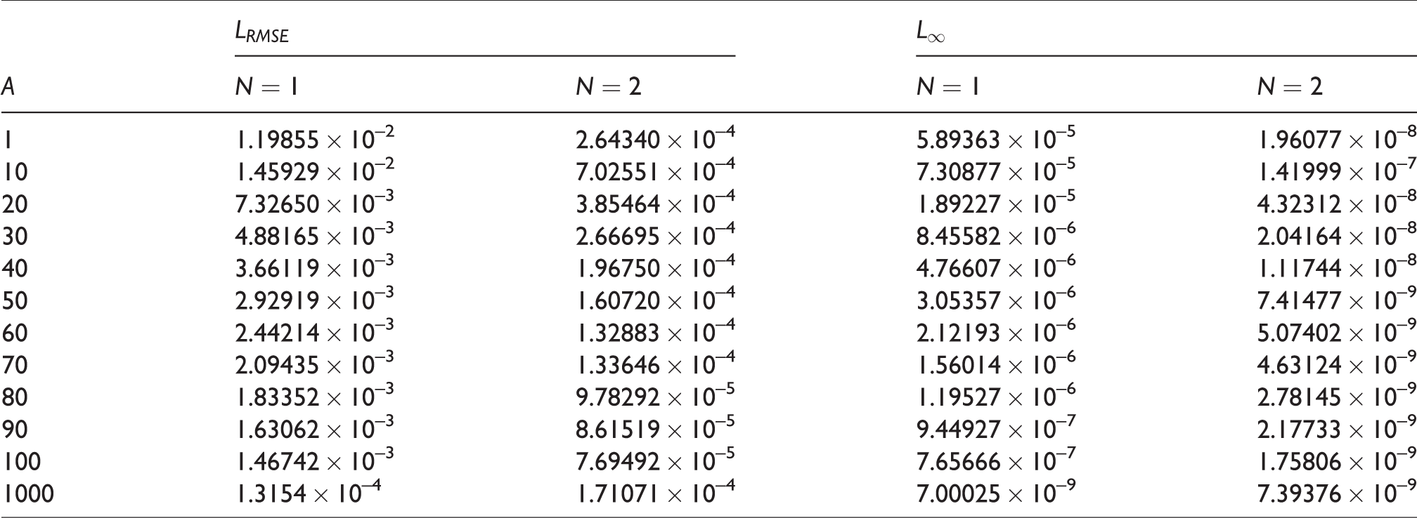
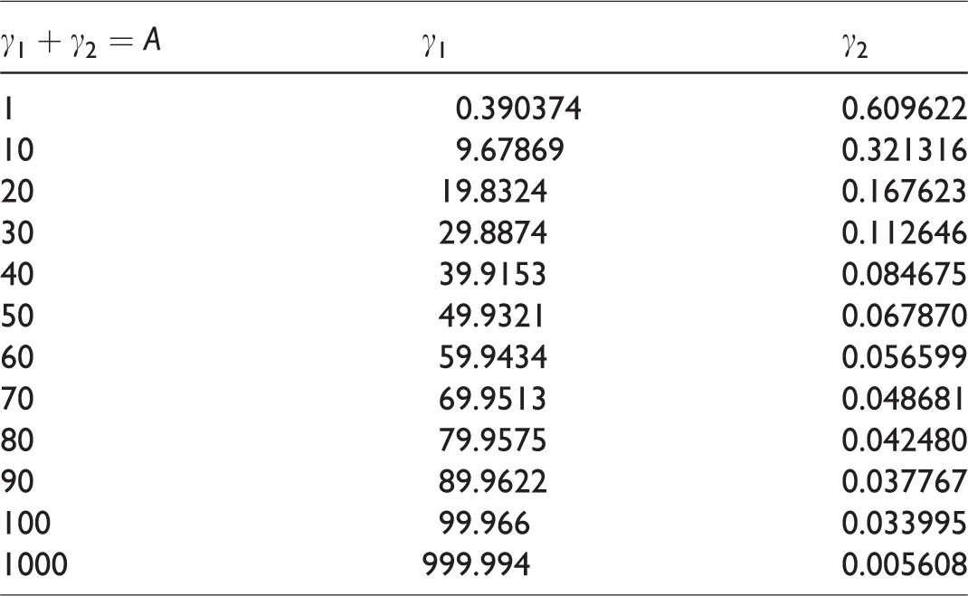
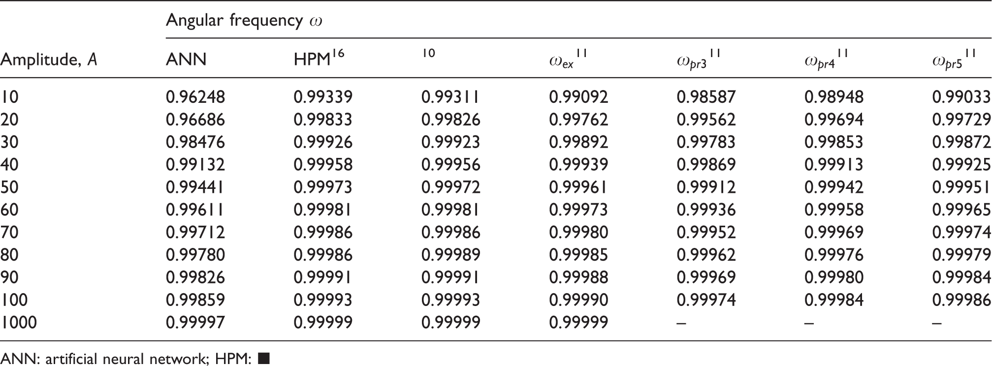
Applying the procedure mentioned in the ‘Methodological configuration’ section, efficient analytical results are attained for $i = 1, 2$ . Table 1 shows the minimum values of the error function $E$ , defined in equation (4), which elaborates the accuracy of the method for a small number of weights of ANN. The values of $E$ are obtained for a large range of amplitude, i.e. $1 < A < 1000$ , of which few of them are depicted in Table 1. It also justifies the positive effect of $A$ on the solution, i.e. for fixed values of neurons $N$ , as the value of amplitude $A$ increases the lesser the minimum value of $E$ is achieved, which on the other hand indicates the higher accuracy of the approximated solution $\hat{Y}$ . Furthermore, Table 2 illustrates some other measurements of error functions, namely, root mean square error $L_{R M S E}$ and mean absolute error $L_{\infty}$ . These functions also define a gradual decrease in values as the value of amplitude $A$ increases. The optimized weight of ANN and comparative results of relation between $A$ and $ω$ are described in Tables 3 and 4, respectively, where the oscillating values of angular frequency $ω$ can be seen clearly at the different values of $A$ . In this table, the optimized values of $A$ are mapped out using equation (13) the sum of two optimized weights $γ_{1}$ and $γ_{2}$ , which in turn generates optimized values of $ω$ . Moreover, Figure 2(a) to (c) is the pictorial representation of the error function $E$ for different values of $A$ , with respect to $t$ , whereas Figure 3(a) to (c) describes several harmonically oscillating motions of the solutions $\hat{Y}$ for various values of $A$ and $ω$ . The dynamical behavior of the nonlinear Duffing oscillator is accomplished by plotting a phase portrait trajectories of the solution $\hat{Y}$ for $A = 80, 90, 100, 1000$ , which is shown in Figure 4.

Figure. 2

(a) to (c). Curvy shapes of fitness function $E$ attained from the proposed method for different values of $A$ , $ω$ and $l = 1, 2$ .

Figure 3.

(a) to (c). Oscillatory solutions of $Y (t)$ attained from the proposed method for different values of $A$ , $ω$ and $l = 1, 2$ .

Figure 4.

Phase plane trajectory of Duffing-harmonic oscillator for $A = 20, 30, 40, 50, 60, 70, 80, 90, 100$ and $l = 1, 2$ .

Table 1.

Minimum values of fitness function $E$ for different calculated values of $A$ , $t \in [0, 1]$ and $l = 1, 2$ .

$A$	$N = 1$	$N = 2$
1	3.65320 × 10^–4	5.73342 × 10^–7
10	6.25183 × 10^–4	4.44681 × 10^–6
20	1.70460 × 10^–4	1.38123 × 10^–6
30	7.70112 × 10^–5	6.39225 × 10^–7
40	4.35690 × 10^–5	3.64717 × 10^–7
50	2.79587 × 10^–5	2.34946 × 10^–7
60	1.94439 × 10^–5	1.63740 × 10^–7
70	1.42979 × 10^–5	1.20696 × 10^–7
80	1.09530 × 10^–5	9.24314 × 10^–8
90	8.65761 × 10^–6	7.31022 × 10^–8
100	7.01462 × 10^–6	5.92534 × 10^–8
1000	7.02288 × 10^–8	3.04108 × 10^–8

Table 2.

Computed values of root mean square and mean absolute error of error function $E$ for different calculated values of $A$ , $t \in [0, 1]$ and $l = 1, 2$ .

$A$	$L_{R M S E}$		$L_{\infty}$
$A$	$N = 1$	$N = 2$	$N = 1$	$N = 2$
1	1.19855 × 10^–2	2.64340 × 10^–4	5.89363 × 10^–5	1.96077 × 10^–8
10	1.45929 × 10^–2	7.02551 × 10^–4	7.30877 × 10^–5	1.41999 × 10^–7
20	7.32650 × 10^–3	3.85464 × 10^–4	1.89227 × 10^–5	4.32312 × 10^–8
30	4.88165 × 10^–3	2.66695 × 10^–4	8.45582 × 10^–6	2.04164 × 10^–8
40	3.66119 × 10^–3	1.96750 × 10^–4	4.76607 × 10^–6	1.11744 × 10^–8
50	2.92919 × 10^–3	1.60720 × 10^–4	3.05357 × 10^–6	7.41477 × 10^–9
60	2.44214 × 10^–3	1.32883 × 10^–4	2.12193 × 10^–6	5.07402 × 10^–9
70	2.09435 × 10^–3	1.33646 × 10^–4	1.56014 × 10^–6	4.63124 × 10^–9
80	1.83352 × 10^–3	9.78292 × 10^–5	1.19527 × 10^–6	2.78145 × 10^–9
90	1.63062 × 10^–3	8.61519 × 10^–5	9.44927 × 10^–7	2.17733 × 10^–9
100	1.46742 × 10^–3	7.69492 × 10^–5	7.65666 × 10^–7	1.75806 × 10^–9
1000	1.3154 × 10^–4	1.71071 × 10^–4	7.00025 × 10^–9	7.39376 × 10^–9

Table 3.

Optimized values of weights of ANN $l = 1, 2$ .

$γ_{1} + γ_{2} = A$	$γ_{1}$	$γ_{2}$
1	0.390374	0.609622
10	9.67869	0.321316
20	19.8324	0.167623
30	29.8874	0.112646
40	39.9153	0.084675
50	49.9321	0.067870
60	59.9434	0.056599
70	69.9513	0.048681
80	79.9575	0.042480
90	89.9622	0.037767
100	99.966	0.033995
1000	999.994	0.005608

Table 4.

Comparison results for ANN, HPM and other methods, for the amplitude $A$ and angular frequency $ω$ , of the Duffing-harmonic oscillation for $l = 1, 2$ .

	Angular frequency $ω$
Amplitude, $A$	ANN	HPM¹⁶	¹⁰	$ω_{e x}$ ¹¹	$ω_{p r 3}$ ¹¹	$ω_{p r 4}$ ¹¹	$ω_{p r 5}$ ¹¹
10	0.96248	0.99339	0.99311	0.99092	0.98587	0.98948	0.99033
20	0.96686	0.99833	0.99826	0.99762	0.99562	0.99694	0.99729
30	0.98476	0.99926	0.99923	0.99892	0.99783	0.99853	0.99872
40	0.99132	0.99958	0.99956	0.99939	0.99869	0.99913	0.99925
50	0.99441	0.99973	0.99972	0.99961	0.99912	0.99942	0.99951
60	0.99611	0.99981	0.99981	0.99973	0.99936	0.99958	0.99965
70	0.99712	0.99986	0.99986	0.99980	0.99952	0.99969	0.99974
80	0.99780	0.99986	0.99989	0.99985	0.99962	0.99976	0.99979
90	0.99826	0.99991	0.99991	0.99988	0.99969	0.99980	0.99984
100	0.99859	0.99993	0.99993	0.99990	0.99974	0.99984	0.99986
1000	0.99997	0.99999	0.99999	0.99999	–	–	–

ANN: artificial neural network; HPM: ▪

Conclusion and future recommendation

In this endeavor, we studied a systematic approach using ANN together with the FFA for Duffing-harmonic oscillator. Consequently, the following outcomes are achieved from the whole study:

Achievement of the main objective of this attempt, i.e. procured accurate solutions of Duffing harmonic-oscillator for wide range of amplitudes, $1 < A < 1000$ with error less than $10^{- 6}$ .

Successful implementation of ANN demonstrates the applicability of ANN on nonlinear dynamical equations to get oscillatory solutions for a small number of neurons.

The activation of artificial neurons of ANN is performed by taking cosine function comprising the angular frequency of the oscillation that has not been considered in the literature yet.

Optimization of the system, to attain the values of unknown weights of ANN, which is magnificently carried out by FFA, elaborates a new application of recently constructed bionic algorithms.

Amalgamation of both efficient methods comes up with a remarkably proficient scheme for all intents and purposes of mathematical models in different fields of science and engineering.

Analytical solutions are beneficial to study any model in multiple ways, i.e. compactly, graphically or in a tabular form. Here, the proposed methodology provides not only an analytically optimized solution but also an optimized association of angular frequency $ω$ and amplitude $A$ .

In future, some more bio-inspired optimizing algorithms will be considered to solve and study different characteristics of differential equations occurring in vast areas of science, engineering, and biology. These algorithms merged with other existing methods enable the solution of every type of differential models including, but not limited to nonlinear, delay, and partial differential models. Henceforth, these schemes will be used to solve nonlinear differential equations of dynamical systems.

Footnotes

Acknowledgements

All the authors are grateful for the comments of the referees.

Declaration of conflicting interests

The author(s) declared no potential conflicts of interest with respect to the research, authorship, and/or publication of this article.

Funding

The author(s) received no financial support for the research, authorship, and/or publication of this article.

References

Khnaijar

Benamar

A discrete model for nonlinear vibration of beams resting on various types of elastic foundations. Adv Acoust Vibr 2017; 2017: Article ID 4740851.

Saetta

Rega

Modeling, dimension reduction and nonlinear vibrations of thermo mechanically coupled laminated plates. Proc Eng 2016; 144: 875–882.

Amabili M. Reduced-order models for nonlinear vibrations, based on natural modes: the case of the circular cylindrical shell. Philos Trans R Soc A: Mathematical, Physical and Engineering Sciences 2013; 371. DOI: 10.1098/rsta.2012.0474.

Chen

, et al. Modified Runge-Kutta method for solving nonlinear vibration of axially travelling string system. In: The 21st international congress on sound and vibration, Beijing, China, 13–17 July 2014, vol. 5, pp. 3896–3901.

Hasrati

Ansari

Torabi

A novel numerical solution strategy for solving nonlinear free and forced vibration problems of cylindrical shells. Appl Math Model 2018; 53: 653–672.

Hoffmann

Liebich

Characterization calculation of nonlinear vibrations in gas foil bearing systems: an experimental and numerical investigation. J Sound Vibr 2018; 412: 389–409.

Zhong

Tang

Hamiltonian approach to Duffing-harmonic equation. Int J Nonlinear Sci Numer Simul 2010; 11: 43–46.

JH.

Hamiltonian approach to nonlinear oscillators. Phys Lett A 2010; 374: 2312–2314.

Ren

ZY.

Theoretical basis of He's frequency-amplitude formulation for nonlinear oscillators. Nonlinear Sci Lett A 2018; 9: 86–90.

10.

Mickens

RE.

Mathematical and numerical study of the Duffing harmonic oscillator. J Sound Vibr 2001; 244: 563–567.

11.

Chen

YZ.

Multiple-parameters technique for higher accurate numerical solution of Duffing-harmonic oscillation. Acta Mech 2011; 218: 217–224.

12.

Syam MI, Raja MAZ, Syam MM, et al. An accurate method for solving the undamped duffing. Int J ApplComput Math 2018; 4: 69.

13.

Duan

JS.

The periodic solution of fractional oscillation equation with periodic input. Adv Math Phys 2013; Article ID 869484.

14.

Mohyud-Din

Iqbal

Hassan

SM.

Modified Legendre wavelets technique for fractional oscillation equations. Entropy 2015; 17: 6925–6936.

15.

Khan

Riaz

Khan

NA.

Parameters approach applied on nonlinear oscillators. Shock Vibr 2014; Article ID 624147.

16.

JH.

Homotopy perturbation method for nonlinear oscillators with coordinate dependent mass. Results Phys 2018; 10: 270–271.

17.

Pakdaman

Ahmadian

Effati

, et al. Solving differential equations of fractional order using an optimization technique based on training artificial neural network. Appl Math Comput 2017; 293: 81–95.

18.

Malek

Bedokhti

RS.

Numerical solution for high order differential equations using a hybrid neural network-optimization method. Appl Math Comput 2006; 183: 260–271.

19.

Munir A, Manzar MA, Khan NA, et al. Intelligent computing approach to analyze the dynamics of wirecoating withOldroyd 8-constant fluid. Neural Comput Appl 2017. DOI: 10.1007/s00521-017-3107-4

20.

Mall

Chakraverty

Comparison of artificial neural network architecture in solving ordinary differential equations. Adv Artif Neural Syst 2013; 2013: Article ID 181895.

21.

Yang

XS.

Nature-inspired Optimization Algorithm. Elsevier, Luniver press, 2014.

22.

Yang

XS.

Firefly algorithm, stochastic test functions and design optimization. IJBIC 2010; 2: 78–84.

23.

Khan

Razzaq

Hameed

, et al. Numerical scheme for global optimization of fractional optimal control problem with boundary conditions. Int J Innov Comput Inform Control 2017; 13: 1669–1679.

Intelligent computing for Duffing-Harmonic oscillator equation via the bio-evolutionary optimization algorithm

Abstract

Keywords

Introduction

Methodological configuration

Intelligent approximation

Fitness function

FFA

Error bounds and convergence

Frequency–amplitude relationship

Homotopy perturbation method

Simulation and results

Conclusion and future recommendation

Footnotes

Acknowledgements

Declaration of conflicting interests

Funding

References