
Abstract
When investigators monitor effects on a population of cells following a perturbation, these events rarely occur in a classical normal (or Gaussian) distribution. A normal distribution is, however, explicitly assumed for events within a single well, in which mean values per well are used as an assay metric and, in general, measures of assay robustness, such as the Z’ score and the V factor. Such analysis is not possible for many technologies; however, high-content screening (HCS) measures events of individual cells, which are averaged over the well. These individual cell-level measurements may be analyzed separately. This study quantifies the extent of nonnormality in experimental samples and their effects on determining the EC50 of a test compound and the assay robustness statistics. The results, based on five sets of publicly available data, indicate that the Z’ or V-factor score can be improved by as much as 0.44 more than standard calculations, and the EC50 of a dose–response curve can be lowered by as much as fivefold when nonparametric methods are used, but not all data sets show a significant improvement. The effect on analysis depends in part on whether the greatest shift from normality occurs in the upper or lower range of the dose–response curve.
Keywords
Introduction
The advent of image-based screening has greatly expanded the range of cell-based assays available to researchers in academia and drug development. 1 These assays include screens for novel phenotypes and workhorse assays for determining compound potency.2–4 These assays operate through image analysis of single cells to quantify cellular responses; however, the cell-level data are usually averaged over the whole well, frequently with additional measures, such as the standard deviation for the cells in the well. The relevance of such measures assumes the cellular responses are normally distributed, and therefore the mean and standard deviation represent accurate summaries of the cellular responses for a given sample. In cases in which the distribution of the sample populations has been examined, however, it has frequently been observed that the data are not normally distributed.5–7 This is largely because cells will respond to a perturbation among a wide range of values or even as subpopulations. 8 Instead of recognizing this as a property of cells in culture, nonhomogeneous responses are usually ascribed to outlier cells that are distinct and not relevant to the general population of cells, and their effects are minimized through the use of statistical measures that are less sensitive to rare events. The most common is to use the median value as the definition of the response for a well, and the corresponding measure of the variance, the median absolute deviation (MAD).9,10 Yet the differences from normality can be severe, and in such cases the use of robust parametric statistical tests may not be entirely sufficient. In such cases, the use of nonparametric statistical tests may be required.11,12
High-content screening (HCS)—or, more generally, image-based screening—represents a richer data set than other well-based measurements such as fluorescence- or luminescence-based enzyme assays that are also performed in microtitre plates.1–4,13,14 Events occurring within a well are interpreted through image analysis as events per cell. The assay metric can be a highly specialized signaling event, such as the phosphorylation of a kinase substrate or the translocation of a receptor or transcription factor. These events may be immediately proximal to the target being manipulated, creating a specific cell-based corollary to a biochemical assay. Controls for the assay can be equally specific and performed as a multiplexed assay, such as a similar protein that should not be affected by the perturbation if it affects the intended target selectively. Last, and most relevant for this study, HCS is uniquely different from these alternative assay technologies, because HCS reports values for a well after measuring events on the individual cells within each well. As such, the measurements for all the cells in a well are reduced to a single (average) number for each well. HCS captures additional statistics for the well, such as the standard deviation of the cellular measurements for each well. The central caveat to this approach is that the mean and standard deviation are statistical measures of normally distributed data, and no assessment is made of the extent to which the data are actually normally distributed. In point of fact, cells in culture are highly heterogeneous; this heterogeneity is an intrinsic and reproducible property of cells in culture and has the potential to affect the interpretation of experimental results.6,7
Operationally, image-based screening (or HCS) is concerned with the identification of cellular perturbations, such as screening for potential therapeutics, and typically relies on the cellular measurements to be averaged for the well (or “well-level” measurements), but this aggregate of “cell-level” measurements can be measured directly, such as by comparing histograms. Although used infrequently, cell-level measurements are calculated during image analysis and can be saved or exported for study (DNA content as a measure of cell cycle distribution is one exception). Studying experiments at the cell level allows for confirmation that the average value is appropriate (which expects that the data are normally distributed) and provides the basis for using methods appropriate to nonnormally distributed data when this is observed. Heterogeneity of cellular populations can occur when discrete subpopulations are present in a sample (such as the presence of stem cell–like tumor progenitor cells), but the transition from a normally distributed sample to the presence of a true subpopulation is not static, and highly skewed distributions can be functionally heterogeneous, even if they are genetically homogeneous. 15 Furthermore, if the skewing changes among samples within the course of an experiment, some statistical tests and assumptions will be incorrect and potentially misleading. In such cases, even if the causes of cellular heterogeneity are not understood, a high level of skewing and changes in the extent of skewing can lead to heterogeneity of variance among samples, or heteroskedasticity.
The principal challenge for a scientist who wishes to understand the distributions that underlie well-level data and whether there is a potential for misinterpretation based on unusual distribution patterns is to rapidly identify such cases as a part of day-to-day activities. Furthermore, the measurement of the deviation from normality needs to be placed in the context of how selecting a particular method of analysis affects experimental conclusions. What are the practical consequences of a lack of normality, and, specifically, would it cause candidate compounds to be ranked differently, or would it cause small interfering RNAs (siRNAs) for a gene to be scored inappropriately, affecting the number of false-positive or false-negative genes reported in a screen? Are there cases in which some skewing in the sample is the result of the inclusion of a minor population of biologically irrelevant outliers and can be disregarded (as is the case when median values for a well are used instead of the mean), or does the lack of normality indicate that the population is truly heterogeneous, and the use of mean or median values fails to account for biologically relevant complexity? The methods outlined in this article allow the rapid assessment of plate-based assays for normality, map the degree of normality by well (allowing a quick visualization of where the lack of normality is greatest), and quantify the impact of using nonparametric statistical tests on assay metrics. Using these methods, a set of publicly available image sets, representing a wide variety of experiment types, has been evaluated.
A secondary challenge is to learn how to equate cellular heterogeneity observed in culture with the role of cellular heterogeneity in developmental and disease biology. Efforts to reduce cellular heterogeneity can affect the experimental system itself (such as interactions between the mechanism of cell-cycle replication block, for the purpose of synchronizing a population of cells, and the perturbation under study). Instead, cell-level approaches have been used to study signal transduction in native populations through flow cytometry and HCS.7,16,17 Such approaches reduce the experimental manipulations that can interfere with the experiment. In addition, and perhaps more to the point, cellular heterogeneity is an intrinsic part of many biological processes, including maintenance of the pluripotent state of a colony of stem cells and the growth of some tumor types such as glioblastomas, which develop subpopulations of cells expressing different receptor tyrosine kinases and interact through paracrine-signaling pathways.18,19
Methods are described in this article that provide such an assessment, and can do so in a rapid and flexible manner. Included in the calculations are measures of mean and median and additional measures of normality, including three goodness-of-fit tests. These methods described here are written to be readily usable by researchers who possess a very small amount of programming experience. The routines do expect data to be entered in a microtitre-plate format (with well locations) but can accept any formatting of the wells, including partial plates. Metadata to assign wells to doses or other treatments (such as RNA interference (RNAi) reagents) can be added to analyses through an additional file. The routines are provided as source code and can be incorporated into other data-processing routines.
Materials and Methods
Experimental Data Sets
All data sets analyzed in this study are publicly available through the Broad Bioimage Benchmarking Collection 20 (BBBC; http://www.broadinstitute.org/bbbc/), including both the images and the metadata explaining the experiments. The image-analysis algorithms are included in these files and specify how the images were corrected for background and other image aberrations, intensities calculated, and features recorded. Image sets were donated and uploaded after being reviewed for image-capture quality, including minimal background aberrations and no saturation. Background problems are frequent but do not necessarily confound image analysis, because there are many methods to correct them, and in fact many algorithms include a background-correction step routinely. Saturation can affect image analysis as well. The dynamic range is instrument specific but is at least 4000:1 (and is approaching 25,000:1), so the dynamic range of the assay itself is typically not the problem; instead, saturation typically occurs when the image-capture settings are based on negative controls or a limited set of perturbations. When saturation is significant, population dynamics such as those explored in this study can be highly compromised, and, indeed, any experimental study will suffer. For population studies, the presence of saturation would be readily detected through an overrepresentation of maximal values (e.g., a strong spike for values in the highest bin in a histogram). Additional technical issues are discussed at the BBBC site, where the image sets can be obtained.
Statistical Analysis Using the R Programming and Visualization Environment
The R programming language was downloaded from one of several mirror sites that provide the language free of charge. Sites are listed at the Comprehensive R Archive Network (http://www.cran.r-project.org).
21
Several supplemental packages are required for these studies, and they are also located at the mirror sites. These packages are nortest,
22
moments,
23
drc,
24
ggplot2,
25
and gridExtra.
26
The analytical and visualization functions they provide are listed in the
Results
Cellular Properties Quantified by HCS Are Nonnormally Distributed
This study looks at sets of publicly available image-based screening data for the purpose of extracting generalizable trends and observations regarding the analysis of image-based cellular assays. Such benchmarking studies have limited use to the general scientific audience if the data or methods are difficult to obtain. Because of this, Ilya Ravkin and members of the Broad Institute Imaging Platform initiated a repository of image sets for image-analysis benchmarking studies that are intended to be used for evaluating imaging applications and methods.
20
These data sets make benchmarking studies much more transparent, because they provide a common set of experiments that can be studied by researchers striving to improve data-analysis methods. Data sets used in this study are described in
Plotting a sample distribution against what the distribution would be if it followed a normal distribution is one of the easiest and most powerful methods for assessing normality. The plot, known as a quantile–quantile (or Q–Q) plot, is used routinely to evaluate data. A quantile is any regular interval of the data range, frequently a percentile but also a quartile or the mean (e.g., the 50th percentile or the second quartile). Nonnormality is readily observed by a deviation of the points from the line. Usually, deviations from normality are small, and the line is a diagonal. To initiate the characterization of HCS data, wells from various experiments were examined using Q–Q plots. Examples are shown in Figure 1 . In these examples, no well of data is truly normally distributed (which occurs when all points lie on the line), although in some cases the data are nearly normally so. The majority of data from an HCS experiment are, however, grossly nonnormally distributed, as the other examples in Figure 1 show. In the cases in which there is significant discordance with a normal distribution, using a parametric statistical test, or even using the mean as the value reported for that well, may be inappropriate.
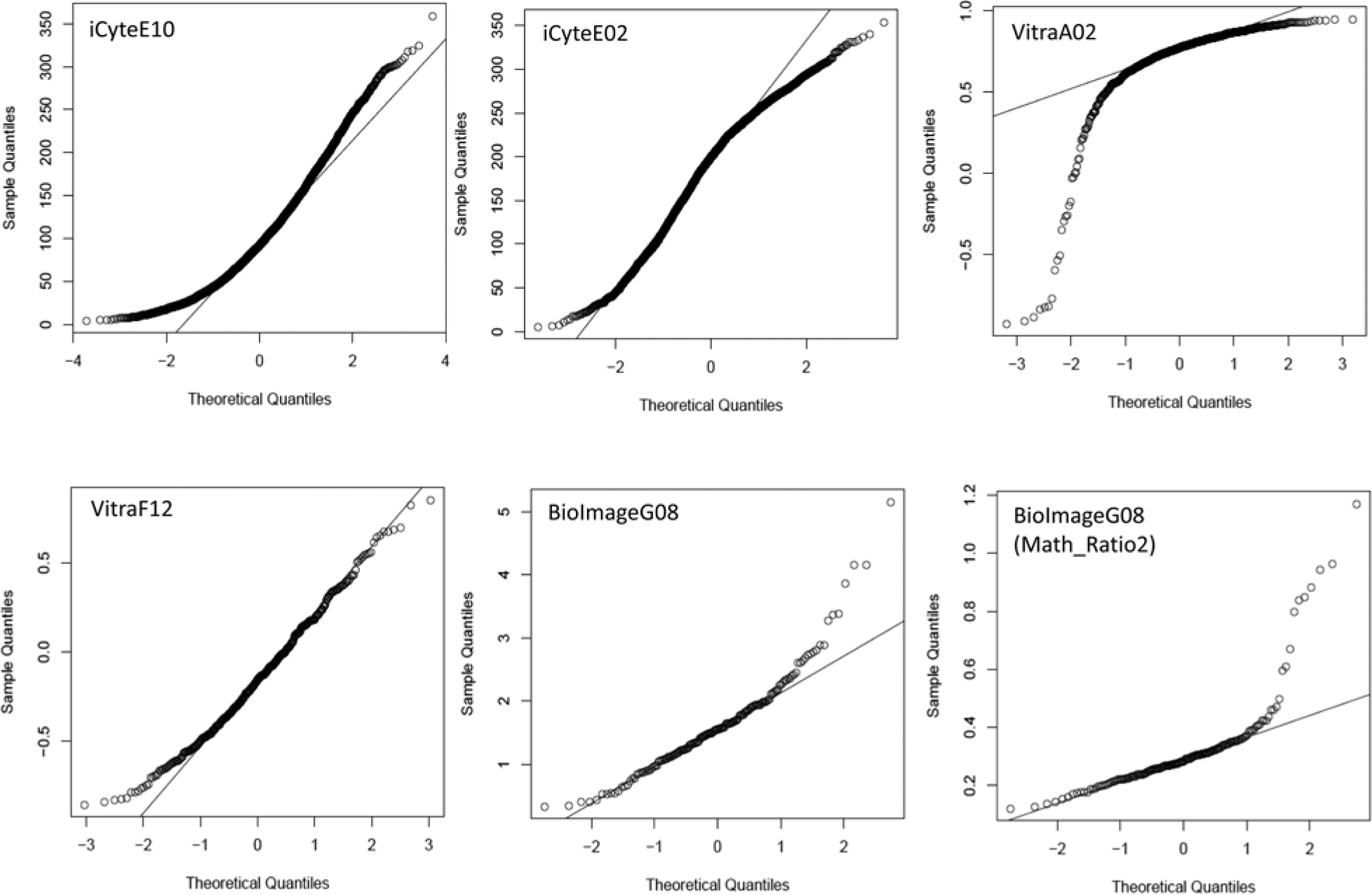
Quantile–quantile (Q–Q) plots of cell-level high-content screening (HCS) data. Data from individual wells of several HCS experiments are plotted by their actual values (identified as sample quantiles along the y-axis) as a function of what the values would be if the data followed a normal distribution. For each data point, the actual value reported (the sample quantile) is plotted against where it should be if the data were to follow a normal distribution. Because both axes are plotted from low to high values, the data are effectively rank ordered. In a normal distribution, the majority of the data points will fall near the mean, or midpoint, of the axes. If a distribution fails to follow a normal distribution, many of the points will not follow this expectation and will therefore fall off of the line (which would be a diagonal if the data were normally distributed). Data shown in the panels are the relevant metric for the indicated well for each experiment, as listed in
Moreover, the patterns of nonnormality in HCS data are varied. Some samples show upward curvature in both the low and the high values, indicating a rightward skew in the data (well E10 of the BBBC–iCyte experiment) or a downward curvature at the tail, indicating a leftward skew in the data (well A02 in the BBBC–Vitra data set is a particularly strong example). The extent of nonnormality is affected by the feature or metric being examined for a well of cells. The figure shows two metrics for well G08 from the BBBC–Bioimage data set. The algorithm measures the translocation of the FOXO transcription factor when treated with PI3K inhibitors, and two metrics that can be used to evaluate the effects of the compounds in the algorithm developed by the Broad Institute Imaging Platform are Math_Ratio1 and Math_Ratio2. These metrics are inversely related measures of the extent of nuclear localization.
Statistical Characterization of Nonnormality in HCS Data
Having noted the lack of normality in HCS data when examined in individual wells, several questions follow, including: How widespread is this lack of normality, how severe is it, is it affected by experimental or control treatments, and does it have a material effect on experimental results? To begin the process of evaluating these questions, the data sets described above were all evaluated using several well-recognized measures of normality. Three statistical tests for normality are commonly used: the Kolmogrov–Smirnov goodness-of-fit test (KS-GoF; essentially, a KS test that compares a sample to a normal distribution), the Anderson–Darling goodness-of-fit test (AD-GoF), and the D’Agostino–Pearson omnibus test (DP-O) for normality. The KS-GoF test is the first widely used test for normality, but the latter two are preferred by statisticians; the AD-GoF test is more sensitive to differences in the tails of a distribution; and the DP-O is a composite of measures for skewness and kurtosis.
27
In this study, the DP-O test was not performed directly, but skewness and kurtosis were evaluated individually. To accomplish this, scripts were written in the R statistical programming language.
21
The language is well developed and includes supplemental packages that extend the power of the language. Several of these packages were used in this script, including the goodness-of-fit tests, as well as graphical routines for presenting the results. A complete list of packages and routines used in this project is detailed in the
These tests are very powerful, and, as indicated in
Figure 1
, all samples show some degree of nonnormality. Although some samples are highly nonnormal, not all samples would be classified as such according to either the KS-GoF or AD-GoF test. Examples from several of the data sets are shown in
Because a lack of normality appears to be a common occurrence and, in at least some cases, an alternative method of analysis may be more statistically proper, there is a need to analyze HCS experiments for normality quickly. Toward this end, a method for characterizing normality within samples in a plate-based assay has been developed. The wellstats script generates two files. The first is a table that lists all the wells of the experiment for the parameters listed above (KS-GoF, AD-GoF, skewness, kurtosis, and the p values for the GoF tests) and is referred to as the wellstats table.
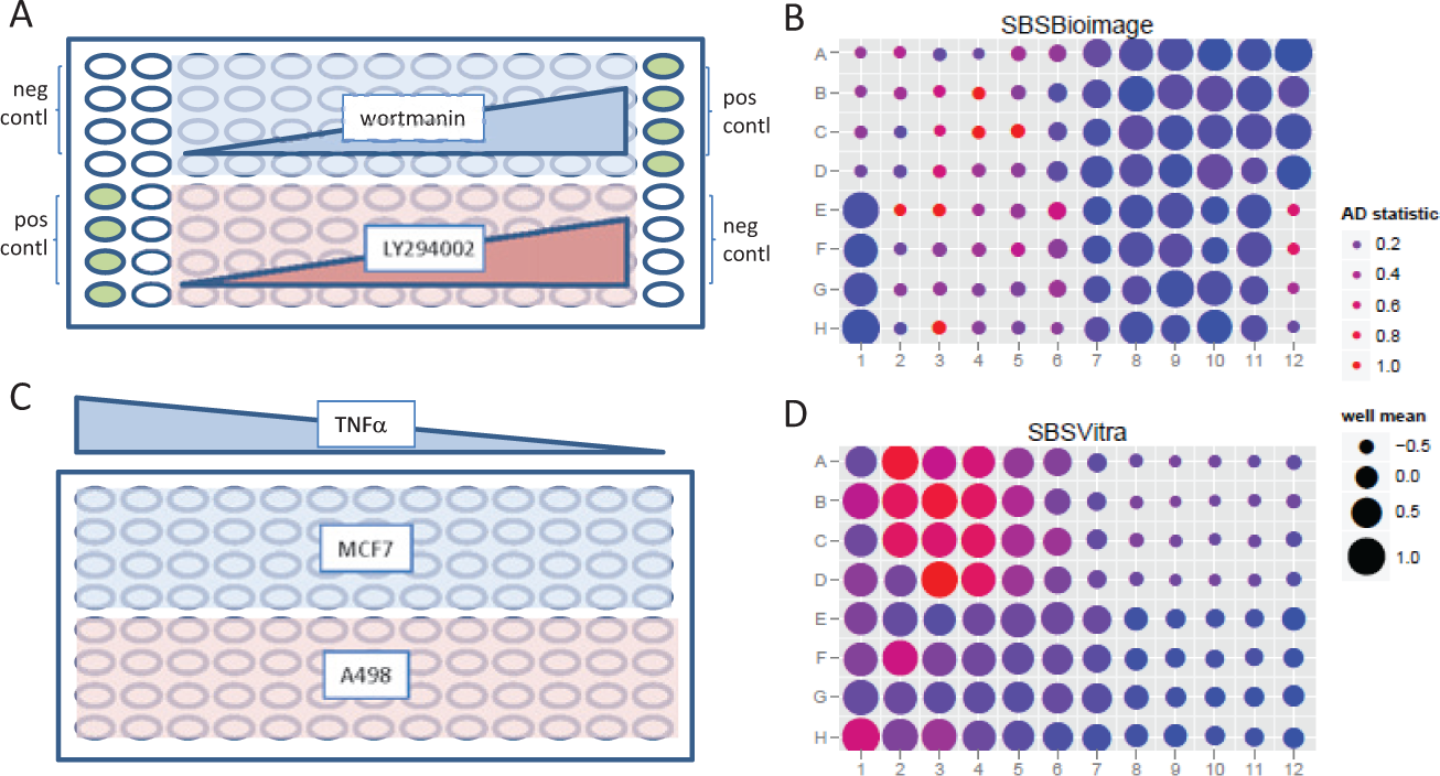
Assessment of normality in high-content screening (HCS) data sets. (
The dependence of nonnormality on dose in the dose–response assays was examined further. For these experiments, the relationship between skewing and kurtosis was evaluated. Results are plotted in Figure 3 . Two patterns can be observed. In the first ( Fig. 3A ), some samples show a positive skew, whereas others show little skew. As concentrations increase, all samples show a shift to more negative skewing, either reducing the initial positive skew back to normal or making a shift to negative skewing in the samples that were initially neutral. Kurtosis is strongly correlated with skew, and either increases as skew increases in the cases in which skewing was initially neutral, or decreases as skewing decreases in the samples that were initially positively skewed, as seen in Figure 3B . The relationship between skewing and kurtosis as a function of dose is further compared in Figure 3C . Skew and kurtosis are related, so it is not surprising that a function between the two is observed in the figure, but what is also observed is the extent to which samples track along this relationship as a function of increasing dose, from positive skewing, to relative normality, to negative skew. Examples of skewing and kurtosis are shown in the remaining panels of the figure. Figure 3D shows the distribution of values for well G04 of the BBBC–Bioimage experiment (plotted on the right side of the skewness–kurtosis plot in Fig. 3C ). This was a sample of U2OS cells treated with a low dose of the PI3K inhibitor LY294002. This sample shows positive skewing in the analysis described above. These MCF7 cells were treated with the highest concentration of TNFα and show a high level of negative skewing. Figure 3E shows well F12 of the BBBC–Vitra experiment, in this case showing A498 cells at the lowest concentration of TNFα. As noted previously, this sample shows a distribution that is much closer to normally distributed than other HCS data. In the last example is well A02 of the BBBC–Vitra experiment, in which negative skewing can be seen in the distribution plot shown in Figure 3F .
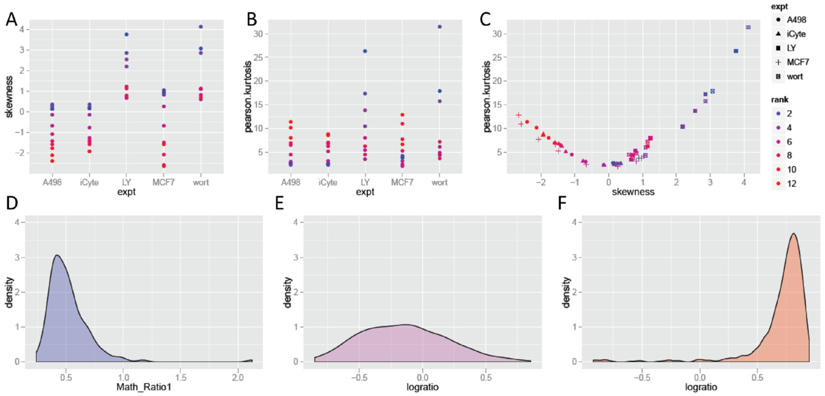
Skewing and kurtosis as functions of assay treatments. (
The effect of the skewing in the distribution curves on the measurement of the well-level responses is examined in more detail in Figure 4 . In Figure 4A , the dose–response relationship is presented for one row of the MCF7 cells in the BBBC–Vitra experiment in the top row, and the BBBC–Bioimage experiment in the second row. In the case of the BBBC–Bioimage data, a sharp peak for the distribution in the initial doses becomes a flatter peak as the doses increase, with some heterogeneity that can be detected.
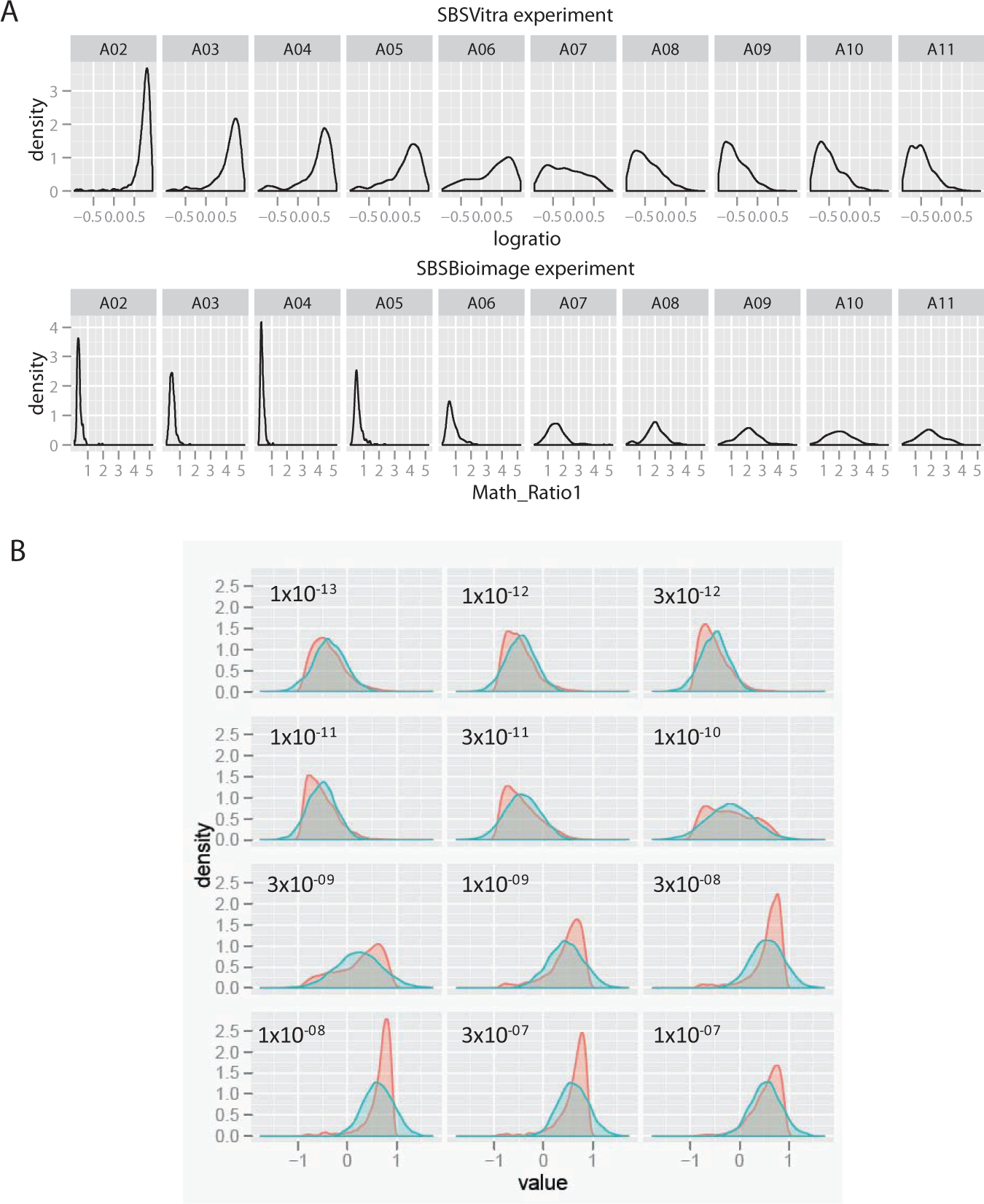
Distributions of actual treatment samples and their corresponding normal distributions, based on parametric values. (
In Figure 4B , density plots for the four replicates of the TNFα-treated MCF7 cells are plotted in red. For each dose, the well-level mean and standard deviation were determined. Taking these parameters, normal distributions were calculated, and these were plotted as density plots in blue. Thus, in each panel, the actual distribution of cells can be compared to a corresponding normal distribution. This is not an idealized normal distribution, but an actual data table; rerunning the procedure will generate a new data set that is normally distributed around the same mean and standard deviation. The assumed normal distribution is able to track the change in NF-κB localization as the dose of TNFα increases, but it misses much of the complexity in the distributions, and generally underreports the degree of change, because the normal distribution is to the right of the majority of the sample values (including the mode) of the actual distribution in the lower concentrations and to the right in the higher concentrations. Thus, at a minimum, using measurements that assume a normal distribution reduces the assay window in this experiment (the extent of the change caused by the treatment). In addition, some heterogeneity may be present, and the compound may not have a uniform effect on the cells, as can be observed in the doses near the middle of the dose–response curve, particularly 1×10⁻¹⁰ M and 3×10−09 M TNFα, in which strong shoulders or possible multiple peaks can be observed. Whether these represent stable subpopulations can be determined through clustering. 28 The mean for the distribution only reports on the center of the peak, but not its shape, meaning that although the assay can be quantified as a move in the mean value as the dose increases, it does not fully report on the events at the cellular level, whereas a nonparametric assessment would be better able to capture the complexity of the response.
Effects of Nonparametric Methods on the Z-Prime and V-Factor Screening Statistical Benchmarks and EC50 Measurements
Because the effect of increased nonnormality is greatest near the EC50 dose, but concentrated on either the lower half or the higher half of the midpoint, it is possible that this will have an effect on the assay statistics, including determination of the EC50 itself. The extent to which this is true was examined. Parametric and nonparametric methods were used to calculate the response of cells in culture to various perturbations. To make these assessments, a second script was written to extend the normality analysis described in
Figure 2
to incorporate dosing information and to measure these effects on standard parameters for assay performance and EC50 calculations. It takes the same feature data used in the first script and generates a new table that reports on normality measurements for doses and replicates, and a plot that compares the dose–response curves for the data when evaluated by well means, t test, and KS statistic; the latter two compare an individual well with the pooled samples in the negative-control wells. In addition, the graphical output reports the Z’, V factor, and EC50 for each of these methods. These provide a per-experiment capacity to examine the extent of nonnormality and its effect on an experiment without significant data manipulation. To provide a comprehensive assessment, a platemap and a plot of the skewness-to-kurtosis relationship are also included. The complete analysis is presented as a dashboard; an example is shown in
Figure 5
. The output from this script calculates and displays the platemap described above, because most experiments are based on a platemap design that is meaningful to the experimenter. In addition, the metadata provide a context for the experiment that can be used to assess the effect of nonnormality on the experiment. This includes mapping the doses to the skewness–kurtosis plot, which helps to orient the extent of nonnormality to the treatment dose. The effects of the parametric and nonparametric measures on the dose–response curve are shown in
Figure 5
. The graph illustrates that there is a pronounced effect on the dose–response curve when analyzed by either the KS test or the t test. As to which one is ultimately selected, additional data, such as the Z’ and V factors, can also be considered, which is why these data are included in the dashboard. The script also generates a
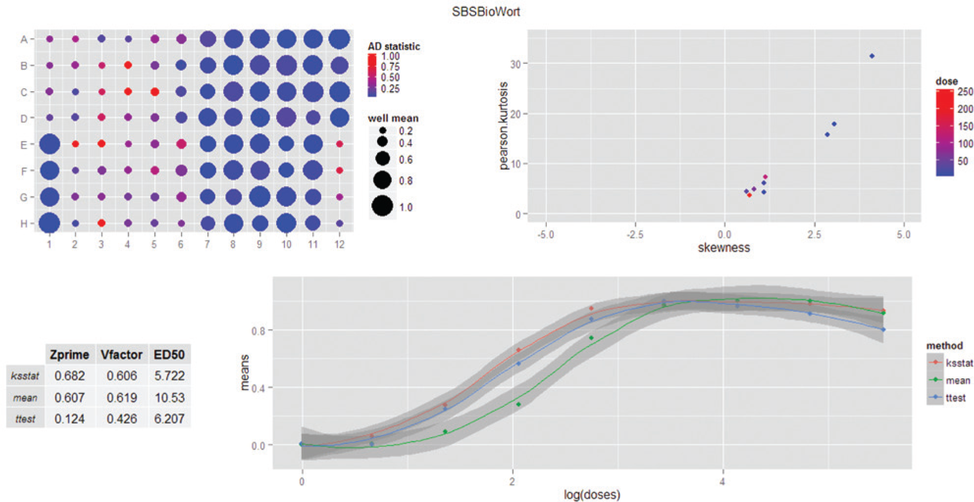
Example dashboard showing analysis of a data set for deviation from normality in the cell-level data. Because this figure is of a dashboard created by the analysis software, it is not a figure of individual panels but is a single figure generated as output. Elements are, from right to left and from top to bottom: (
The standard well-based measurement, the mean value for the well, was compared to both a parametric and a nonparametric comparison of each sample to the control wells. In this case, the KS test was compared to the parametric t test. Although many analytical approaches use the well-mean values for the relevant feature or endpoint, the t test is also used in some cases. 29 For a nonparametric test, the KS statistic is probably the most commonly used in HCS, although the Wilcoxon–Mann–Whitney U test is more directly analogous to the t test. The Wilcoxon–Mann–Whitney U test is a cumulative measure of two samples, whereas the KS is a measure of proportional difference between two scaled distributions. The cumulative nature of the Wilcoxon-Mann-Whitney U test makes it difficult to use for high-content data, because the number of cell-level comparisons is very high (from hundreds to tens of thousands). The test is less linear than the KS test, particularly at the midranges of the dose–response curves, and therefore less useful as a metric. In contrast, the KS test returns a value between 0 and 1, based on the point of greatest divergence between the two populations, which is a much easier metric to use and understand. Like the t test, the p values for both tests also work as metrics if log transformed. Standard deviations are calculated for the differences among replicate wells for each analysis and are plotted in the dose–response curves as shaded regions.
The results for these tests on all of the data sets used in this study are summarized in Table 1 . As can be seen in the table, effects are experiment specific; and because of this, rather than conclude from this study that a specific change in experimental analysis is called for, the exploratory nature of these methods can help an investigator decide if such modifications are in fact called for. In some cases, the effects were negligible, such as the iCyte experiment, for which the samples were largely normal among all of the treatment conditions and there were no changes in EC50, Z’, and V factor. In contrast, changes in Z’ and V factor can be large, more than 0.3 change (the maximum value for these tests is 1.0), and the effect on EC50 ranges can exceed fivefold. The final determination (particularly for the EC50 determination) should be made by taking the data that have been exported to a .csv file, recalculating with the standard laboratory software, and substituting the KS test values or other available measurements as desired, for reasons discussed below.
Screening Statistics for Parametric and Nonparametric Analyses.
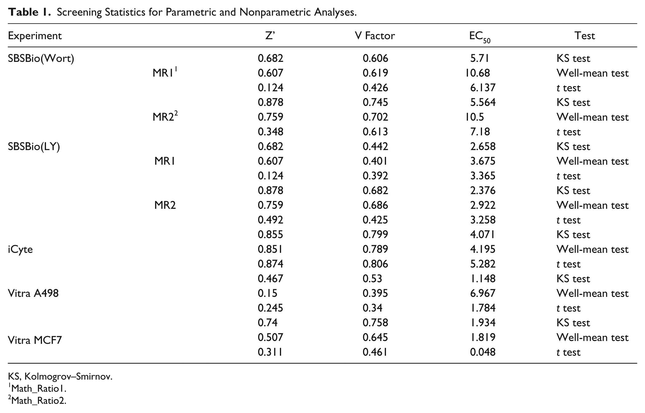
KS, Kolmogrov–Smirnov.
Math_Ratio1.
Math_Ratio2.
One aspect of the dashboard that is important to remember is that it is an aggregate of separate programs. The normality tests, skewness, and kurtosis are described above; the latter two are calculated after pooling the cell-level measurements for replicate wells at each dose. The well-level mean values, t test, and KS test values are for each well and dose; standard deviations are calculated at the well level for each method. From these measurements, the dose–response curves are plotted, including the error measurements. The positive- and negative-control samples are evaluated individually through a comparison with the pooled negative-control samples; these individual values can also be added to the plot or the table in the dashboard. The EC50 calculations are derived from a separate routine and therefore have a potential to be discordant with a visual estimation of the EC50 from the plots. EC50 calculations are notoriously difficult to determine from raw data, in which noise and a failure to completely plateau at the maximal dose have strong effects on the EC50 measurement. 30 In standard studies of compound effects, a failure to reach a definitive plateau in an experiment may trigger a revised experimental design in which the compound treatment doses would increase until such a plateau was reached. In this case, the EC50 calculation is based on the presumption that the maximal dose has been reached, and therefore it could be considered a “forced” EC50 calculation. The decision to handle the data this way is based on the idea that these procedures are exploratory in nature, designed to provide an indication of whether additional studies are warranted.
Software Tools for the Rapid Assessment of Normality in HCS Feature Data
Progress in understanding the effects of the cell-level distribution on experimental conclusions and downstream decisions rests largely on the ability of a scientist to evaluate the data quickly. The methods described here have been written in the form of R scripts that perform the analyses and generate tables and plots to enable a typical researcher to rapidly evaluate data from their experiment. With these data, the experimenter has the ability to decide whether a departure from normality materially affects the conclusion of an experiment. For the experimental metric, either a feature value taken from the cell-level data file (typically, a .csv file) or a calculated value, such as a ratio of two feature values or a feature that has been transformed, a two-column table is loaded into R. A guide for formatting data is included in the
In evaluating high-content data, it is common to examine several features as candidate assay metrics. For example, total nuclear intensity could be compared to the nuclear-cytoplasmic ratio and difference, giving three options for measuring the extent of a nuclear translocation. Phosphorylation of a protein could be evaluated by average intensity per cell or total intensity per cell. In all cases, there are biological reasons why one feature may be more appropriate as well as reasons why multiple features may be redundant for an experiment (such as average and total intensity values for cells that do not change size or shape during the course of the experiment). An additional script is included here that allows the evaluation of four features simultaneously. The script generates wellstats tables for each feature and a single platemap plot for the four features. From this analysis, the feature to be chosen as an assay metric can be further evaluated by the dosestats script. The source code for the dosestats script is provided in the
Discussion
Heterogeneity of cells in culture is generally well appreciated, particularly for cancer cell lines, most of which are highly aneuploid. Such cellular heterogeneity is, however, typically viewed as a population of outliers, and is typically ignored outright or through taking the median value when a population-based method such as HCS is used. Usually, the regression toward the mean is cited as the principle for doing so, with the frequent observation that small samples may show nonnormality, but that as sample size increases, the population assumes a normal distribution. To limit the impact of this sampling-based appearance of nonnormality, the median is used instead of the mean.
These results suggest that nonnormality is an accurate reflection of cellular heterogeneity and is evident in many experiments. Although not the case for all experiments, statistical heterogeneity, particularly variability in the variance of the population, can affect experimental conclusions. For experiments exhibiting severe nonnormality, using a nonparametric test is a demonstrably more sensitive analytical approach. In such cases, the first population of cells that respond to a compound may be a robust indication of critical compound properties, such as the ability of the compound to penetrate cells and hit the target. In contrast, the mean may infer a state that is not represented at the cell level at all. Toriello and coworkers 31 showed that GAPDH mRNA levels in cells treated with an siRNA were strikingly bimodal; expression levels in 50 cells analyzed at the single-cell level were either 50% or 0% of control. The arithmetic mean of 22% of control did not actually occur in any cell. Sisan et al. 6 showed that GFP expression is bimodal across a 300-fold range and that sorting cells from high or low GFP expression levels and following them in culture would eventually give rise to the original distribution, leading to the conclusion that such a bimodal distribution is a true property of the cells in culture and is not captured by the average value for the population. 6
The data routines have focused on the development of a single dashboard as a vehicle for exploratory data analysis. Dashboard visualizations continue to grow in importance in the era of “Big Data,” as multiple sets of data need to be reviewed together before a conclusion can be made. For cell-level data generated in HCS experiments, the effect of the analytical method should be considered, and the current version of the dashboard ties assessments of normality on standard experimental measurements, including the EC50, with visualizations of how deviations from normality vary with treatment dose. From these data, a decision can be made on whether the standard well-level measurements based on average cellular responses are appropriate or whether an alternative approach should be considered. One thing that is clear from the analyses performed in this study is that there is an experiment-by-experiment decision, because some experiments show little (or at least inconsequential) deviation from normality, whereas others can show up to a 10-fold change in EC50 value and increased Z’ or V-factor scores. Because of this, the abilities to quickly review the experiments and do so without being encumbered by a fixed experimental design are important.
Heterogeneity has been shown to be biologically relevant, and the appreciation of its importance in developmental and disease biology is increasing. For example, aggressive glioblastoma is fueled by a mixture of cells expressing multiple receptor tyrosine kinases in a mixed or mosaic pattern that includes EGFR, PDGFRA, KIT, MET, and VEGFRA.18,19 Cellular heterogeneity is also essential for pluripotency and differentiation of stem cell populations, 32 as well as the stratification of liver hepatocytes into gluconeogenic and glycogenolic subtypes through regulated levels of Wnt signaling. 33 Well-level methods that fail to differentiate effects on essential subpopulations miss opportunities to understand the effects of candidate therapeutics. Clearly, as these studies progress, a specific set of disease cells may come to define the critical population, and methods that can focus on events in subpopulations will differentiate durable therapies from other efforts. HCS is well positioned to focus on such subpopulations and cellular heterogeneity in general. In addition to methods of image analysis that can query subpopulations defined by cytological specifications, refined data analysis, such as the methods described here, can focus an experiment on subpopulations defined by response thresholds. In this regard, a certain irony has emerged, in which efforts to study cells have focused on methods to reduce heterogeneity, even when studying diseases in which heterogeneity is an important part of the biology of the system. Methods that account for heterogeneity may in fact provide better models for natural biological processes, including disease progression.
The question of when heterogeneity in a sample can be considered as an aggregate of individual subclasses is one that will require discussion. Currently, methods exist to define many different classes for a cell line.8,34 These result when multiple proteins that show broad independent distributions are sorted (two proteins that independently show high, medium, and low levels can be considered to stratify a cell into nine subpopulations). Comparing this work to that of Sisan 6 suggests that these states could persist throughout several generations. Even cases in which relaxation back to the pretreatment state occurs more quickly can have a material effect on therapeutic response. 35 This has been discussed by Sorger and colleagues, 36 who have observed that heterogeneity of cells within a single cell type can result in a survivor fraction, a transient state that can give rise to increased resistance to the perturbation (TRAIL, in this case) but does not define a fundamentally resistant population and is one that will reset its heterogeneity, much as the GFP level did in the Sisan experiments. 6 This can be a significant disconnect between an assay response at the well level (such as caspase activity) and a treatment effect in the biological context, because the survivor population represents persistence but not resistance at the cellular level, but can nevertheless be a significant cause of treatment failure. This definition is explicitly empirical. Treatment of a therapeutic targeted to mitotic cells for 1 h and then washed out will show a high survival fraction, whereas application of the treatment for 72 h should result in nearly complete killing in culture, increasing the effective homogeneity of the cells in culture. The patterns of protein-level adjustments observed by Plant and Sorger suggest that some therapeutics will show incomplete effects even for longer duration treatment cycles. The potential for these varied and heterogeneous responses can be important for comparing candidate targets or therapeutics. The methods described here can help to identify these behaviors in routine experiments and can alert the experimenter to events that may require more direct follow-up.
Footnotes
Acknowledgements
Lin T. Guey is thanked for several helpful discussions on statistical approaches to high-content data. David Logan provided helpful background on the BBBC image collection and analyses, and Anne Carpenter gave helpful comments on the manuscript; their efforts are also very much appreciated.
Declaration of Conflicting Interests
The author declared no potential conflicts of interest with respect to the research, authorship, and/or publication of this article.
Funding
The author received no financial support for the research, authorship, and/or publication of this article.
References
Supplementary Material
Please find the following supplemental material available below.
For Open Access articles published under a Creative Commons License, all supplemental material carries the same license as the article it is associated with.
For non-Open Access articles published, all supplemental material carries a non-exclusive license, and permission requests for re-use of supplemental material or any part of supplemental material shall be sent directly to the copyright owner as specified in the copyright notice associated with the article.