Automated Analysis and Classification of Infected Macrophages Using Bright-Field Amplitude Contrast Data

Abstract

This article presents a methodology for acquisition and analysis of bright-field amplitude contrast image data in high-throughput screening (HTS) for the measurement of cell density, cell viability, and classification of individual cells into phenotypic classes. We present a robust image analysis pipeline, where the original data are subjected to image standardization, image enhancement, and segmentation by region growing. This work develops new imaging and analysis techniques for cell analysis in HTS and successfully addresses a particular need for direct measurement of cell density and other features without using dyes.

Introduction

Bright-field microscopy is a nontoxic, dye-free technique that uses direct observation of the illuminated objects and is widely used to observe cells under the microscope. A number of studies have been published on the usefulness of bright-field imaging in cell detection and analysis. Although several researchers^1–3 have used phase contrast microscopy to visualize the phase shift introduced by the interaction of light with the objects, these techniques require special objectives and devices. Conversely, bright-field amplitude contrast microscopy does not require special devices, but the image contrast is quite poor due to the transparency of the cells.

Bright-field images in the current study are the result of overall amplitude contrast caused by the cellular objects in the light path. The same image analysis methodology also works well for phase contrast images. Because the cells are generally semi-transparent, and cell organelles are too small to be distinguished clearly with the wavelength of a white light source, the cell images in bright-field data look somewhat like texture patches. Several previous object recognition techniques have attempted to detect and count sf9 cells in bright-field images using active contour models.^4,5 Active contour models do not work satisfactorily in the presence of strong texture and pixel intensity variation, which is a characteristic of the amplitude contrast images. The broader literature review shows that not much work has been done on automatic analysis of bright-field cell data. No work was found on amplitude contrast bright-field images of primary cells in a high-throughput screening (HTS) context. In this article, we propose a set of techniques that will convert the bright-field cytological image data into relatively high-contrast images facilitating the use of region-growing techniques to identify and label individual cells automatically. These were used to calculate hundreds of unbiased features for each segmented cell. We have demonstrated the utility of the method in counting the number of macrophages and classifying them as infected and uninfected based on the phenotypic measurements.

Material and Methods

Monocyte-Derived Macrophage Culture

Negatively selected, apheresed CD14-positive monocytes were thawed quickly at 37 °C and washed in complete media. Complete media consisted of RPMI 1640 (HyClone, Logan, UT) supplemented with 10% fetal bovine sera (FBS; Sigma, St. Louis, MO), 2 mM L-glutamine (Invitrogen, Carlsbad, CA), 40 U/mL GM-CSF (R&D Systems, Minneapolis, MN), and 100 U/mL M-CSF (R&D Systems). Cell density was adjusted to 7 × 10 ⁵ cells/mL, and 50 µL of cell suspension (35 000 cells) was added to each well of a 384-well Cell Carrier plate (PerkinElmer, Waltham, MA). Plated cells were incubated at 37 °C in humidified atmosphere with 5% CO₂ for 24 h. Typical monocyte adherence was 25% to 30%. Media were replaced 24 h and 96 h postplating. Cells were differentiated for a total of 7 days.

On day 7, monocyte-derived macrophages (MDMs) were infected with Francisella tularensis ΔblaB::GFP, a Ft LVS mutant that stably expresses green fluorescent protein (GFP) integrated into the chromosome under the control of a constitutive promoter at a multiplicity of infection (MOI, bacteria/cell) of 100. MDMs and bacteria were incubated at 37 °C/5% CO₂ for 2 h to allow for phagocytosis, after which unincorporated bacteria were removed by washing 3 times with Hank’s buffered saline solution (HBSS). Infected cells were incubated at 37 °C and 5% CO₂ for 50 to 72 h.

After fixation, the cells were washed once in HBSS and stained with final concentrations of 1 µM Cell Trace BODIPY TR methyl ester (Invitrogen), 0.25 µg/mL Cell Mask Deep Red (Invitrogen), and 1 µM final Hoechst (Sigma) in HBSS. MDMs were stained for 30 min at 37 °C in humidified atmosphere with 5% CO₂. After staining, the cells were washed in HBSS and incubated in 1% bovine serum albumin (BSA) in phosphate-buffered saline (PBS; Thermo Fisher, Waltham, MA) for 20 min at room temperature or 37 °C. Cells were washed and stained with 165 nM final concentration of BODIPY 650/665 phalloidin (Invitrogen) prepared in PBS and 1% BSA for 30 min at room temperature or 37 °C. Cells were washed again, and 50 µL of PBS containing 1 µM Hoechst was added to each well. Each stain used in this protocol provides specific textural information of different cellular components.

Image Acquisition

An Opera Confocal imaging system (www.cellularImaging.com/products/Opera) was modified with a simple blue LED flashlight hung over the 384-well plate to act as a bright-field light source. First, the bright-field images were collected from all of the preselected image fields in a well, and then the same image fields were reacquired in fluorescent mode by scanning over the well a second time. Although there is a shift in the cell locations between bright-field imaging and fluorescent imaging due to slight movement of the well-plate before fluorescent imaging, one can visually ascertain the common cells between the same field of view in bright-field and fluorescent images. Although the flashlight light source is unreliable and the image quality from such a locally modified system is very poor, it serves the basic HTS purpose of cell density estimation and general feature measurement if another bright-field imaging system is unavailable in the lab. Approximately 5000 infected cells and 5000 control cells were collected for each sample analyzed. Images were collected with a 40× water-immersed objective with a numerical aperture (NA) = 0.9. The pixel intensities were binned by a factor of 2 during the camera-level quantization, resulting in images of 20× magnification with improved signal-to-noise ratio.

Image Analysis

The general image analytics flow diagram to detect and classify the cells is shown in Figure 1 . Image analysis methods were divided into image enhancement, cell segmentation, feature measurement, and classification. The main reason for the failure of the traditional segmentation technique on the amplitude contrast data is that at a higher resolution, the data are highly textured due to uneven light absorption by the cellular ultra-structures, and the background is bright and noisy.

Figure 1.

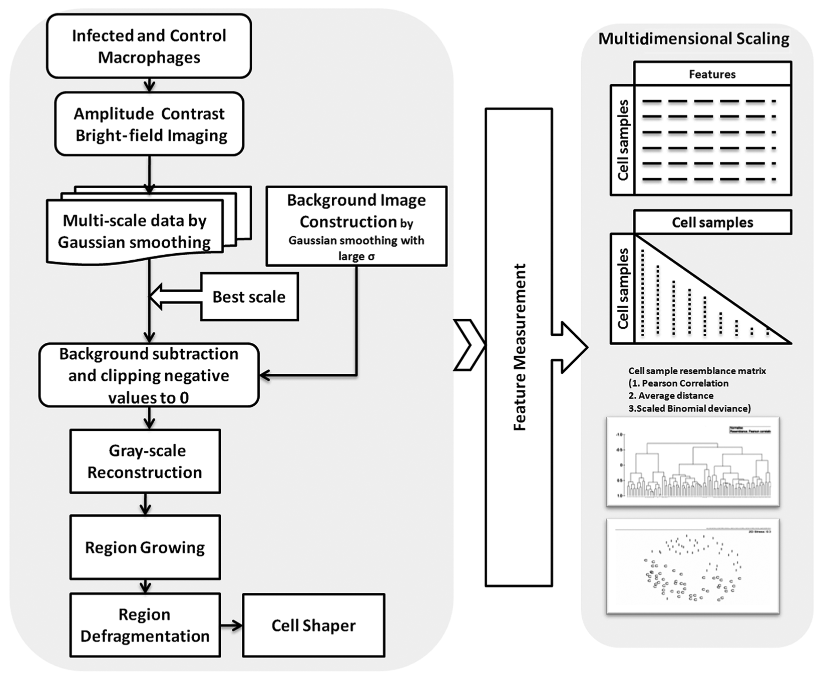
Control flow diagram of bright-field cell image analysis process.

Image Enhancement

The first step in the image enhancement is the application of a sequential pipeline of filters such as gradient magnitude image generation, smoothing, histogram equalization, and image recombination, followed by gray-level scaling, in that order. The goal here is to transform the image to a different scale where most of the higher frequency information that is not required for the segmentation is reduced and the background is converted to a darker low-intensity region. The brightness and the smoothness of the cellular region that facilitates better cell segmentation are simultaneously enhanced by the filtering process.

Let I(x, y) be the input image function that shows image pixel intensity I at pixel location (x, y). The discrete gradient magnitude map of I(x, y) is given by

$$g(x,y)=\sqrt{{(I(x-1,y)-I(x+1,y))}^2+{(I(x,y-1)-I(x,y+1))}^2}$$

(1)

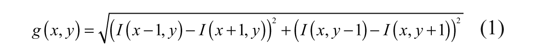
Apply histogram equalization on the gradient magnitude image g(x, y). Histogram equalization fundamentally tries to redistribute the gray level such that the resulting data have a flatter histogram. In practice, this enhances the brightness of the objects in the image. Let g_eq be the histogram-equalized gradient magnitude image and G(x, y) be the Gaussian-smoothed g_eq with σ = 21. The σ value is selected based on experiments with a small set of data. For any new data that are very different in quality from the small set of experimental data, one may have to reset the σ appropriately.

The contrast-enhanced image I_eq is given by

$$I_{ce}=\frac{(I(x,y)\cdot G(x,y))-\text{MIN}(I(x,y)\cdot G(x,y))}{\text{MAX}(I(x,y)\cdot G(x,y))-\text{MIN}(I(x,y)\cdot G(x,y))}\times \text{MAX}(I(x,y))$$

(2)

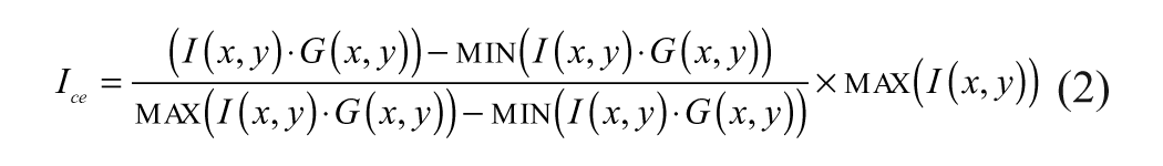
Figure 2A shows an example image, and Figure 2B shows the contrast-enhanced image by the above method. The contrast-enhanced image is further smoothed to reduce the pixel intensity offshoots, noisy dark patches, and so on within the cell regions.

Figure 2.

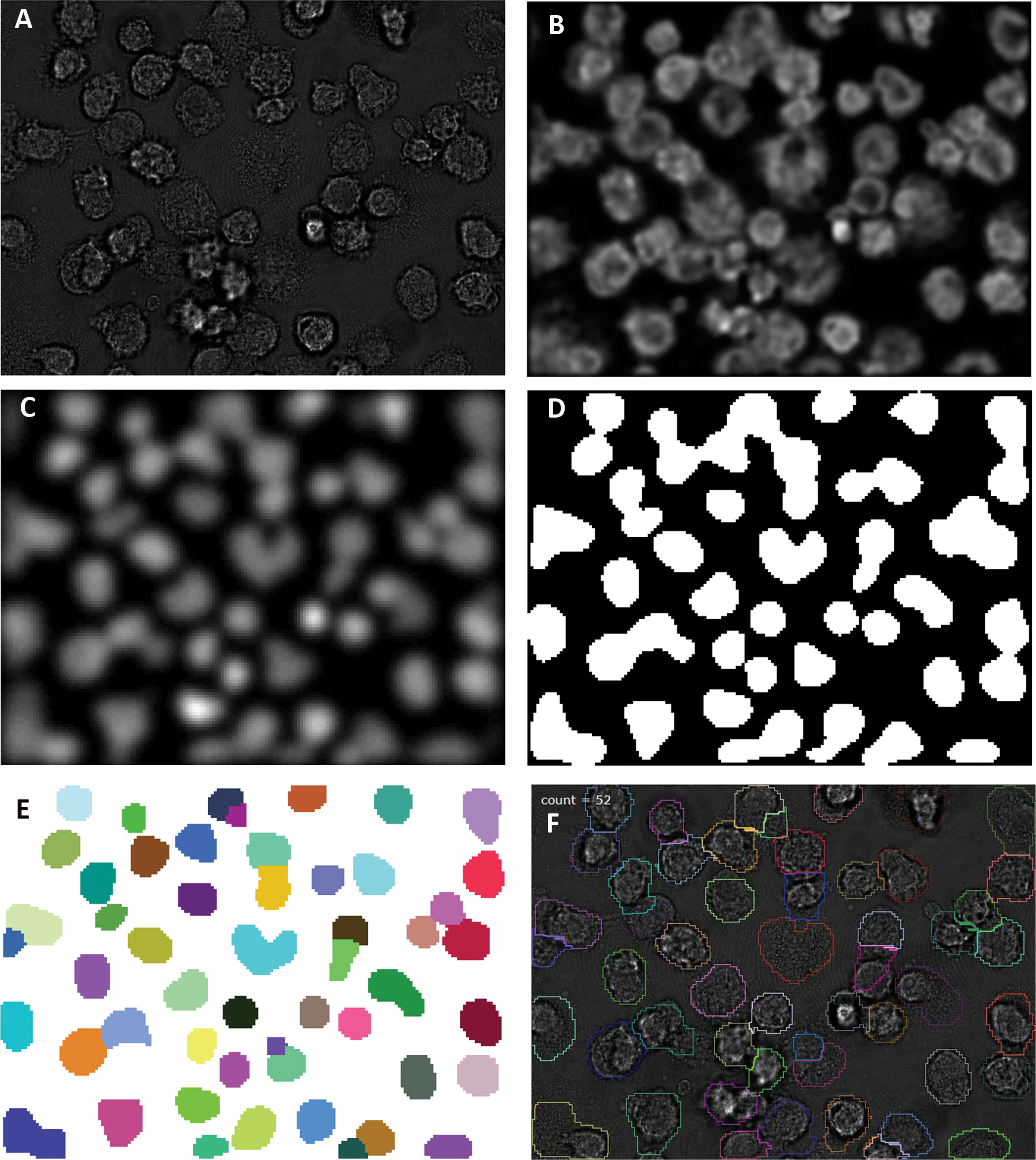
(A) Original bright-field amplitude contrast image (B) after contrast enhancement and (C) after background subtraction and all stages of preprocessing have been completed. (D) Binary mask by minimum error thresholding. (E) Result of segmentation. (F) Masks are dilated by two pixels to correct for watershed and the boundary of the masks superposed on the original image.

In the second step, background intensity variation is reduced. This is accomplished by reconstructing a background image as a very low-frequency version of the contrast-enhanced image. The background image is then subtracted from the contrast-enhanced image. The negative values are clipped to zero, and the result is rescaled. The resulting image is further diffused using a Gaussian filter (σ = 3) to facilitate binarization. Figure 2C shows a background-suppressed and smoothed foreground image. In general, some form of smoothing is done after every contrast manipulation stage to reduce the undesired effects of contrast manipulation. The preprocessing filters are used to manipulate the images and standardize the image quality and the pixel statistics in such a way that a consistent input is provided to the segmentation process.

Image Segmentation

The images are thresholded to obtain a global mask with a clear separation of background and foreground pixels using a minimum error thresholding method. ⁶ The holes in the binary image are filled by analyzing the negative binary image where objects under a certain size are considered holes in the positive image, and hence those pixels are restored to foreground intensity in the binary image. Figure 2D shows the result of thresholding by a minimum error method followed by hole filling. A modified watershed algorithm described in Adiga et al. ⁷ was implemented to segment the individual cells from the cluster of touching and overlapping cells. Figure 2E shows the result of a watershed-type region growing on the binary image of Figure 2D . The watershed algorithm uses the modified distance map where Euclidean distance of the foreground pixels is calculated as the distance from the object boundary pixels. This generally results in reduced-size object masks. We dilated the object masks by two pixels to correct for this error, and the mask boundary was superposed on the original data, as shown in Figure 2F .

Despite all the preprocessing efforts and modifications to the watershed algorithm to avoid multiple markers per cell, it is not possible to completely remove the cell fragmentation caused by noisy markers. The noisy peaks near the cell boundary caused by the less than perfect convex surface of the cells would still cause fragmentation of the cell. These fragments are quite small and can be detected by size and shape parameters. To detect the fragments, we have calculated the depth of objects as the maximum distance value within the labeled objects. If this distance value is less than a certain preset distance, the object is considered a fragment. If the depth of an average cell is r pixel units, then the objects whose depth values are less than r/4 pixel units are considered cell fragments. The fragment is merged with a cell that has a longest shared boundary with the fragment.

To demonstrate the utility of bright-field imaging and analysis over fluorescent imaging in the HTS context, we have also acquired data from the same samples in a fluorescent mode using a combination of stains described earlier to highlight nucleus, cell membrane, and many other organelles and membranes in the cell cytoplasm. Figure 3A shows the bright-field image with a segmented boundary superposed on it. Figure 3B shows the corresponding fluorescent image with the segmented boundary superposed. Figure 3C shows the result of segmentation based on the fluorescent nucleus stain (Hoechst). It is observed that some of the cells present in Figure 3B are not represented in Figure 3C because the corresponding nuclei are not visible. The segmentation method used for fluorescent images is the same method used for bright-field data with appropriate parameter tuning to obtain the best possible result. The bright-field and fluorescent images do not perfectly correspond because the well-plate was moved between acquiring the images in two different imaging modes. A few cells are numbered in Figure 3A and Figure 3B to provide the match for the visual convenience. The cells without numbers printed on them are not common to both images.

Figure 3.

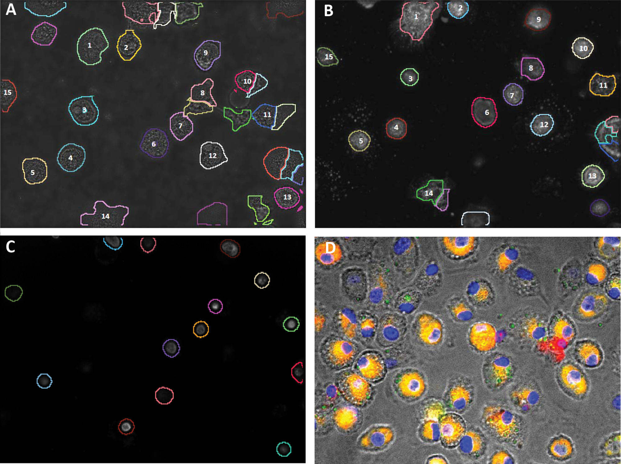
Comparison of segmentation process for a bright-field image and its corresponding fluorescent image. (A) Bright-field image with superposed segmented mask boundary. (B) Fluorescent image with a superposed segmented mask boundary. (C) Segmentation of the same specimen in B using nuclear stain only. The numbered cells in A and B are the corresponding cells in the specimen. (D) An example of the bright-field image superimposed with the corresponding fluorescent image highlighting the possible errors in fluorescentbased image analysis for cellular feature measurement.

Feature Analysis

Bright-field data of macrophages, unlike fluorescent imaging data, do not show any deterministic and/or functional feature(s) that can be used to characterize a cell. It is thus important to quantify all possible features from the cell image and to design a suitable classifier. Cell size, shape features, and their derivatives depend on the scaling and hence are suitably normalized before classification. We have calculated more than 1000 features for each cell image. These features include basic size and shape descriptors, multiscale features, ⁸ invariant moment features, ⁹ statistical texture features, ¹⁰ Laws texture features (statistical texture features of Laws texture images), ¹¹ differential features of the intensity surface (features of local gradient magnitude, local gradient orientation, Laplacian, isophote, flowline, brightness, shape index, etc.), ¹² frequency domain features, histogram features, distribution features (radial, angular, etc. of intensity distribution, gradient magnitude distribution), local binary pattern image features, ¹³ local contrast pattern image features, ¹⁴ cell boundary features, edge features, and other heuristic features such as spottiness, χ ² distance between histograms of pixel patches and between concentric circular areas within the cell, gray class distance, heuristic and problem-specific features, and so on. Features were calculated for each cell and normalized to have a value between 0.0 and 1.0.

Classification

Our classification problem is a simple one. We have to reduce the dimensionality of the feature vector in the first step and find a threshold to classify the objects into two classes. The multidimensional scaling (MDS) introduced by Kruskal ¹⁵ overcomes the inflexibility of principal component analysis (PCA) to use different similarity index poor preservation of interclass (dis)similarity. The purpose of the MDS is to provide a structure for the sample distribution, which attempts to satisfy the dissimilarity matrix constructed from the sample features. We have used Primer software (www.primer-e.com), which provides MDS as one of the data reduction techniques followed by hierarchical clustering to classify the data.

Results and Discussion

To demonstrate the accuracy of the segmentation against manually marked boundaries and against automatic segmentation using the fluorescent data, 100 cells from 50 different images were selected. The accuracy of segmentation can be measured as a percentage of symmetric difference ⁷ in the area of the cell given by automatic segmentation in bright-field data, automatic segmentation in fluorescent data, and the corresponding manual segmentation. If A₁ is the set of all pixels in the cell segmented by method 1 and A₂ is the set of pixels in the cell segmented by method 2, then the percentage of symmetric difference is given by

$$100\times (\{A_1\cup A_2\}\backslash \{A_1\cap A_2\})/(\#A_2)$$

where ∪ is the set union operator, ∩ is the set intersection operator, #A₂ is the number of pixels in set A₂, and \ is the set difference operator.

In bright-field images, the average percentage symmetric difference between an automatically marked cell area in the bright-field images and the cell area in manually marked cells is 11%, with a range of 2% to 16%. The average percentage symmetric difference between a cell area in the manually marked cells and the automatically segmented cells from the fluorescent images is 18%, with a range of 7% to 26%. The higher level of accuracy while using bright-field data instead of fluorescent data is also obvious from the composite image shown in Figure 3D . This composite image shows that staining-based measurement of global features such as size, shape, and so on can be inaccurate.

To analyze the usefulness of the system, we classified features from the images of uninfected control cells and infected cells using MDS. Figure 4A , B shows the MDS ordination plot of more than 400 cells from infected and control wells. Dissimilarity measures, such as Euclidean distance between the cell sample features and binomial deviance, were used to demonstrate that by using a different or problem-specific dissimilarity measure, one can better classify the cell samples in the phenotypic feature space. Large variance among the infected cells is a result of the presence of many uninfected cells and cells at different infection stages in the infected wells. The variance within the control cells is arguably due to inherent structural differences within the same kind of primary cells and also possible error in automatic segmentation of the cells. Figure 4C , D shows the MDS ordination plot of a smaller set of cells that are classified as live (indicated by 0) or dead (indicated by 1). The gold standard for live–dead classification is based on Sytox orange dye. From the feature-based classification shown in Figure 4C , D , one can argue that several cells that are actually marked live due to lack of Sytox staining of the nuclear DNA are very close to the dead cell class center. This can be due to uneven uptake of Sytox orange dye or because cells that are preapoptotic show major features of the dead cells but are not dead at the time of fixing.

Figure 4.

(A) Two-dimensional multidimensional scaling (MDS) ordination plot (MDS component1 along x-axis and MDS component2 along y-axis) of infected and control sample points with (A) Euclidean distance used as a dissimilarity measure (2D stress = 0.09; C, control; I, infected) and (B) binomial deviance used as dissimilarity measure (2D stress = 0.11; C, control; I, infected). (C) Live–dead cell classification with Euclidean distance as a dissimilarity measure (2D stress = 0.15; 1, dead; 0, live). (D) Live–dead cell classification with distance metric as a dissimilarity measure (2D stress = 0.1; 1, dead; 0, live).

In general, we have demonstrated that it is possible to use bright-field amplitude contrast image data to measure cell density and, in certain cases, classify the cells into different phenotypic classes. If image analysis is used for more complex challenges, such as measurement of several cell features, fluorescent imaging requires additional dyes to mark the whole cell region, in addition to the dyes depicting organelles of interest and so on. Because the dyes may not stain the complete cytoplasm as shown in Figure 3D , the morphological and textural features that quantify the cell phenotype can be quite compromised in the fluorescent data. Some of these dyes are toxic in nature, and hence live-cell imaging using these dyes may result in biased data. The process of fixation and staining often adds experimental artifacts to the cell images. By using bright-field data, one can save on the cost of dyes as well as time for multispectral image acquisition and data storage. The reduction in computational cost is straightforward because we are dealing with just one image channel instead of multispectral data. The methodology proposed in this article allows for rapid assay development and actually preserves spectral options for stains if increased dimensionality is desired.

The image analysis routines and feature descriptors are written in .NET framework using C# language, making them widely accessible. The prototype software application will be made available on request after the publication.