Sage Journals: Discover world-class research

Abstract

This article considers the operation of the time series processes that underlie U.S. crime rate trends. These processes are important because they carry the influence of the variables that generate the rates. They limit the forms that explanations of crime trends can take, and they open avenues for new theoretical development. Using data from the nation and a panel of large cities, analysis finds that crime trends operate much like random walks or their smoothed cousins; that they rarely deviate from a constant pattern; and that they show little evidence of nonlinearity. The article discusses the substantive implications of these features for understanding crime trends, and it considers directions for expanding the study of their empirical properties.

Keywords

time series processes equilibria nonstationarity nonlinearity stylized facts

Introduction

The goal of this article is to consider several empirical regularities in crime rate trends. The typical way of studying crime trends is to propose a theory and then test its fit to the data. A less explored approach begins with the trends and tries to discover the structures that underlie them. If successful, the second approach can yield a set of properties that apply broadly to fluctuations in crime and that offer a foundation for theorizing. The article applies this second approach.

An obvious feature of a time series is that it connects values from the past to values in the present. In popular usage, a “trend” is exactly that: a set of observations arranged in temporal order. Using Uniform Crime Report (UCR) data, Figure 1 graphs U.S. homicide, rape, robbery, assault, burglary, and auto theft rates since 1933, and U.S. larceny rates since 1960. The accuracy of the data is always open to question, and the series even now are relatively short. Still, the graphs clearly display significant variations, such as the increases in the 1960s and the drops in the 1990s.

Figure 1.

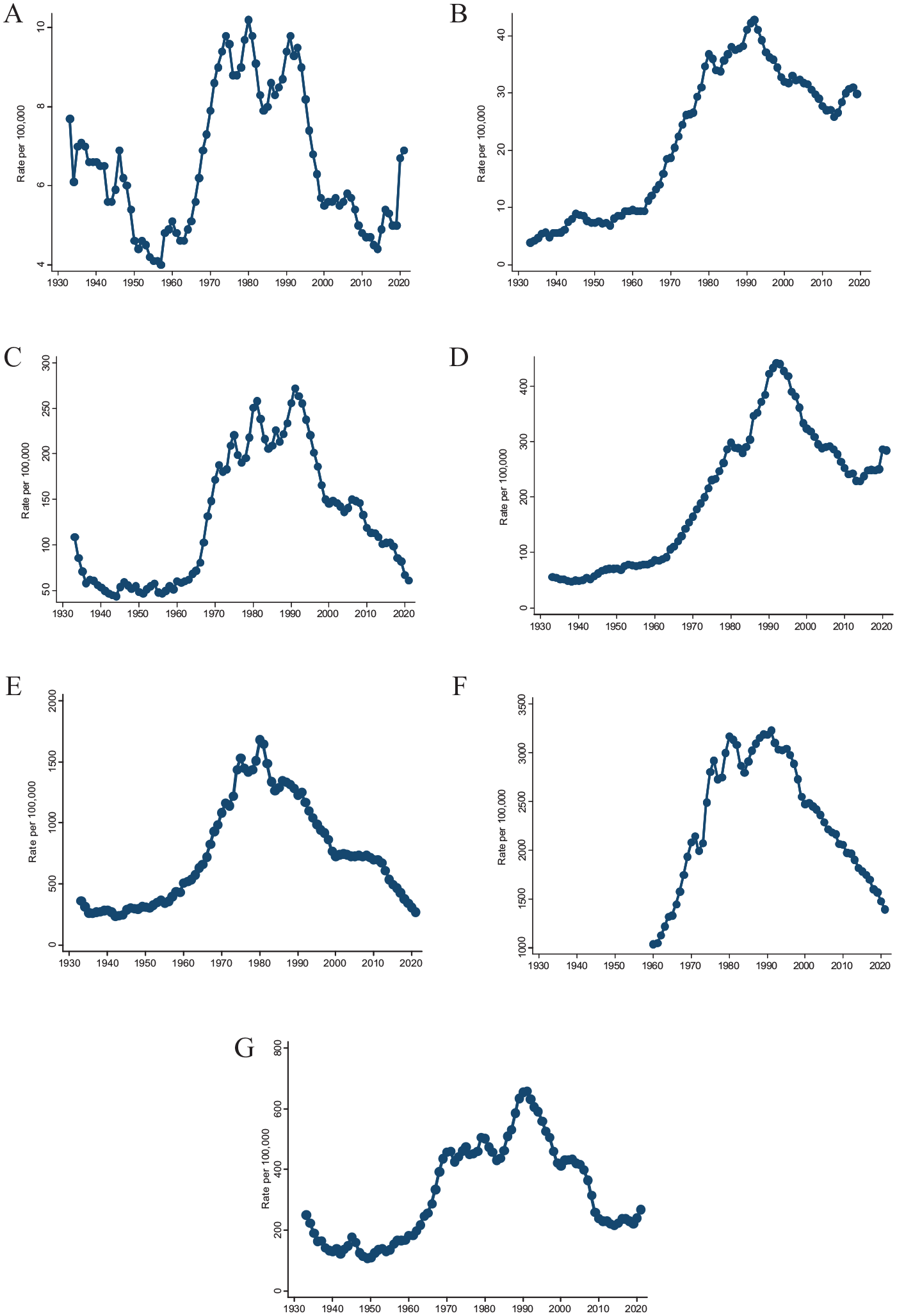
Uniform Crime Report National Crime Rates. (A) Homicide, 1933–2021. (B) Rape, 1933–2019. (C) Robbery, 1933–2021. (D) Assault, 1933–2021. (E) Burglary, 1933–2021. (F) Larceny, 1960–2021. (G) Auto theft, 1933–2021.

The trends are the outcomes of probability processes that underlie the rates. Many processes are possible, differing in how they work. At one extreme, a process may produce a white noise series, where observations have only chance relationships to the ones before and after them. At the other extreme, a process may follow an exacting equation, such as one that produces a linear trend.

Time series processes are not simply abstractions, and instead, they have important practical uses. They allow conventional statistical analyses, for example, by supplying a basis for inference. The process that underlies a time series is the equivalent of the population that underlies a cross-sectional sample, and it justifies the standard statistical procedures and tests.

Equally important, processes constrain and focus theoretical explanations of how a series can vary. Only some forms of change are possible, and the behavior that a theory requires might be incompatible with the process. Some processes do not have constant means, for example, and for them explanations that assume average rates cannot be correct. The same is true of theories that assume rates follow cycles, or are contagious, or shift in their causal structure. A process can support or help rule out large classes of theories because it sets conditions that they must meet.

Knowledge of the generating process can also be helpful in developing theories. A process carries the influence of the causal variables that are ultimately of interest to researchers. It cannot identify these variables individually, especially if they are numerous. Still, it can offer insight into their collective dynamics and into the behaviors of which they are capable. It can address questions such as: What general forms must explanations of crime trends take? What features of the trends are theoretically meaningful? What empirical conditions must a trend theory satisfy?

The current article will investigate some features of the processes that underlie the trends in the major U.S. rates. Researchers have commented on a few of these features in the past, but they have largely ignored others. Even when they have been a topic of earlier study, the substantive implications of the features have not received much discussion.

In the remaining sections, the article first describes the data that form its empirical basis. The following section then goes on to consider the structure of crime trends, separating theory from empirics. The next two sections examine deviations from the temporal structure, especially involving outliers and nonlinearity. The final section discusses the implications of the results for understanding crime trends and for developing a catalog of their empirical properties.

Data

The article relies on two sets of data to illustrate the characteristics that it considers. One set consists of national crime rate series from the UCR. These cover homicide, robbery, assault, burglary, and auto theft between 1933 and 2021, larceny between 1960 and 2021, and rape between 1933 and 2019. The series appear in Figure 1.

The UCR system revised its data collection methods in 1958, and it did not claim national coverage before 1960. Most studies of trends, therefore, begin in 1960, discarding the earlier years of data. Excepting larceny, however, the U.S. Office of Management and the Budget revised UCR data from 1933 to 1959 to conform with the later standards (U.S. Office of Management and the Budget, 1973). The revised data extend the series, and longer series are more useful for examining trends. The quality of the earlier data is nevertheless a matter of concern, and the article points out places where the post-1959 series yields different conclusions.

The FBI also changed its definition of rape in 2013, increasing reported rates. Until 2019 it continued to present rape rates under the legacy definition, however, and the paper uses these for continuity. Accordingly, the rape series ends in 2019.

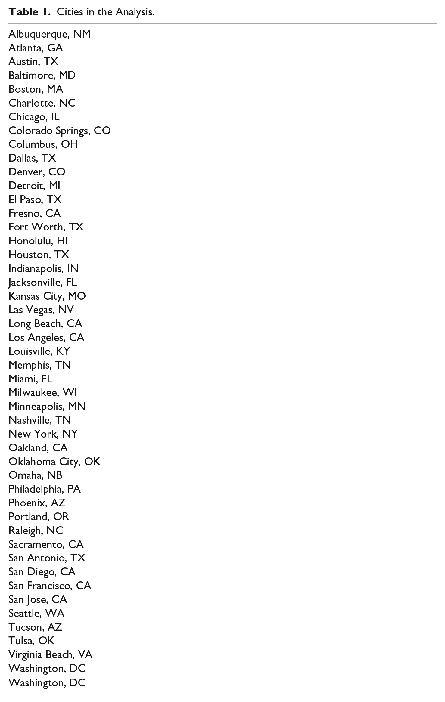
The second set of data is a panel of U.S. cities with 2020 populations of 400,000 persons or more. The panel covers the 1960-2021 period, and Table 1 lists its 47 members. To avoid drowning in detail, the city analysis examines only homicides, the most accurately recorded crime and the one of greatest scholarly and public interest. Panel data have several advantages for the article, increasing the number of observations and allowing the study of heterogeneity in the trends.

Table 1.

Cities in the Analysis.

Albuquerque, NM

Atlanta, GA

Austin, TX

Baltimore, MD

Boston, MA

Charlotte, NC

Chicago, IL

Colorado Springs, CO

Columbus, OH

Dallas, TX

Denver, CO

Detroit, MI

El Paso, TX

Fresno, CA

Fort Worth, TX

Honolulu, HI

Houston, TX

Indianapolis, IN

Jacksonville, FL

Kansas City, MO

Las Vegas, NV

Long Beach, CA

Los Angeles, CA

Louisville, KY

Memphis, TN

Miami, FL

Milwaukee, WI

Minneapolis, MN

Nashville, TN

New York, NY

Oakland, CA

Oklahoma City, OK

Omaha, NB

Philadelphia, PA

Phoenix, AZ

Portland, OR

Raleigh, NC

Sacramento, CA

San Antonio, TX

San Diego, CA

San Francisco, CA

San Jose, CA

Seattle, WA

Tucson, AZ

Tulsa, OK

Virginia Beach, VA

Washington, DC

The Shape of Crime Rate Trends—Theory

A central feature of a time series process involves its mean and variance. Broadly, two types of processes exist, ones that are stationary and ones that are nonstationary. Stationary processes produce observations that have constant means and variances, while these characteristics are variable if a process is nonstationary. A stationary series fluctuates closely about a mean or a deterministic trend, never straying far from it. A nonstationary series lacks affinity for any specific value and will wander, increasing and decreasing without a discernable pattern.

The series that stationary and nonstationary processes generate require different analytical approaches. If a series is stationary, an analysis of its original levels–its raw values–will yield statistically consistent estimates under the usual regression assumptions. This is also true for series with deterministic linear trends after adding components to control for them. In contrast, analyses of nonstationary series in their levels will be vulnerable to finding spurious relationships, even controlling for deterministic trends (see Enders, 2015). Statistically desirable estimates instead must come from analysis of period-over-period differences rather than levels.¹

Stationary and nonstationary series also require different theoretical explanations. Theories that specify an equilibrium around which crime rates vary must assume that the rates are stationary. In such theories, if crime moves above or below its equilibrium—a mean or a trend line—reactive forces will push it back. A common use of an equilibrium argument is invoking “mean reversion” to explain an unusual increase or decrease in crime (e.g., Harcourt and Ludwig, 2016).

An example of a fully developed equilibrium theory is the idea of a natural crime rate, independently proposed by several sets of economists (Friedman et al., 1989; Narayan et al., 2010; Philipson & Posner, 1996). Analogizing from the idea of a natural unemployment rate, these theories argue that crimes will fluctuate around means set by stable social structures. Changes in criminal justice policies or demographic compositions might temporarily increase or decrease crime levels, but these effects will dissipate over time.

A similar but more distinctively criminological equilibrium theory rests on Durkheim’s (1895/1966) discussion of normal crime rates. According to Durkheim, and like the economists, conditions within a society generate a constant rate of offending. Although crime levels may vary above or below this value, large departures occur only during periods of significant social stress.

Messner and Rosenfeld (2013) expand on Durkheim by situating the source of high US crime rates in the nation’s emphasis on the economy over other social institutions. This institutional imbalance generates persistently high levels of offending that are mostly stable in international perspective. Like Durkheim, however, Rosenfeld and Messner (2010) raise the possibility that in some circumstances rates can move to abnormally high or low levels. They suggest that the declining rates the United States experienced during the 1990s might in fact have been abnormal, the product of mass incarceration and expansionist economic policies.²

In contrast to the well-developed theories that rely on stationary processes, no detailed crime trend explanation rests on nonstationarity. The lack of formal development aside, most trend studies do implicitly assume that crime rates are non-stationary. As already noted, nonstationary series generally provide statistically desirable estimates only after conversion into period-over-period differences. Without modification, the transformation to differences means that relationships between series exist solely in the short term. The levels of external variables in a particular period influence the value of a time series only during that period. If in the next period the external forces change, the series changes with them.

A nonstationary time series does not have an equilibrium that tethers it to a baseline. It does not regress back toward a mean or revert to a trend, and it can become arbitrarily large or small. Depending on the forces that move them, nonstationary crime series can, in theory, increase to levels unheard of in modern societies or fall so low that they essentially disappear. Still, although they can move in the same direction for long periods, they do not consistently trend.

Overall, the sense of a nonstationary series is that its value at a particular time depends on the concurrent values of multiple external variables. Sometimes these variables change by large amounts and sometimes their changes are negligible. Sometimes they collectively work in the same direction, and sometimes they work against each other.

Studies of crime rate trends (e.g., Baumer & Wolff, 2014; Blumstein & Wallman, 2007) usually discuss the trends in language that is compatible with a nonstationary process. They look to current conditions to explain current rates, and they say little about long-term dynamics. The studies do not formally address nonstationarity, however, and so do not take advantage of the insights that it might provide. They also do not allow for nonstationarity in their data analyses, and so risk finding spurious relationships by using the series in their original levels.

The Shape of Crime Rate Trends—Basic Empirics

Many competing “unit root” tests seek to distinguish between stationary and nonstationary time series. Among these, the article will rely on the augmented Dickey-Fuller (ADF) test. The ADF test is not always the best choice (Maddala & Kim, 1998), but it was the first developed and it is highly popular in applications. The test considers three possibilities: whether a series is stationary around a mean, whether it is stationary around a deterministic trend, or whether it is nonstationary. It uses nonstationarity as its null hypothesis.

All analyses in the present article use log transformations of the series. This helps equalize the series variances and gives their changes approximate percentage interpretations. The findings do not, however, depend on the transformations. According to the results (Table 2), the national series for all seven UCR crimes failed to reject nonstationarity, with or without deterministic trends.

Table 2.

Augmented Dickey-Fuller Stationarity Test for National Uniform Crime Report Series.

Null hypothesis: series follows a nonstationary process
	Without deterministic trend	With deterministic trend
Homicide	Z(t) = −1.654, p = .48	Z(t) = −1.644, p = .77
Rape	Z(t) = −2.191, p = .21	Z(t) = −0.593, p = .98
Robbery	Z(t) = −1.092, p = .72	Z(t) = −0.351, p = .99
Assault	Z(t) = −1.720, p = .42	Z(t) = −1.070, p = .93
Burglary	Z(t) = −0.918, p = .78	Z(t) = 0.729, p > .99
Larceny	Z(t) = −1.970, p = .30	Z(t) = −2.317, p =. 42
Auto theft	Z(t) = −1.415, p = .57	Z(t) = −1.482, p = .83

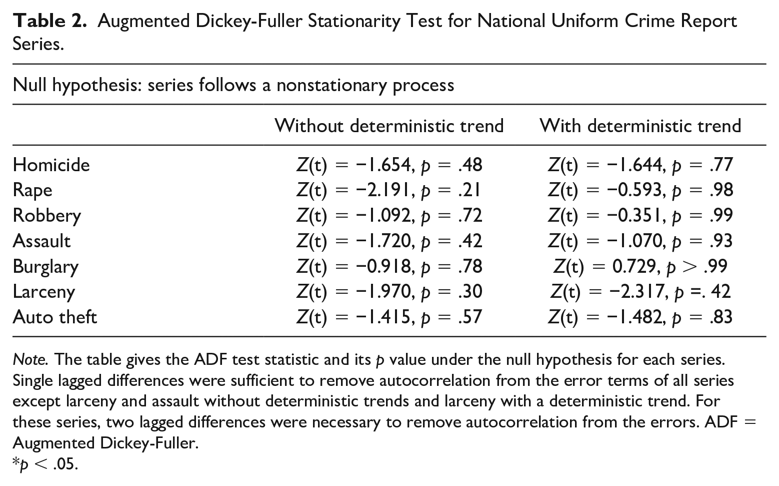
Note. The table gives the ADF test statistic and its p value under the null hypothesis for each series. Single lagged differences were sufficient to remove autocorrelation from the error terms of all series except larceny and assault without deterministic trends and larceny with a deterministic trend. For these series, two lagged differences were necessary to remove autocorrelation from the errors. ADF = Augmented Dickey-Fuller.

p < .05.

For the city panel, two testing options exist. One is to test the null hypothesis that all city series are collectively nonstationary, with the alternative that at least one follows a stationary process. The other is to test each series individually. Because the tests produce a large amount of detail, the results of these analyses appear in the paper’s online Supplementary Material.

Pesaran’s (2015) CIPS test, a collective test that allows for cross-sectional correlations, rejected nonstationarity. Yet by construction, collective tests can reject if only one member of a panel follows a stationary process. Pesaran (2012) accordingly recommended caution in interpreting null hypothesis rejections for entire panels and suggested also testing the series individually.

Applying individual ADF tests to each city, 35 failed to reject nonstationarity, creating a general impression of nonstationarity overall. Six cities did reject: Colorado Springs, Kansas City, Minneapolis, Oakland, Omaha, and Virginia Beach. Six more cities rejected after controlling for deterministic trends: Indianapolis, Las Vegas, Nashville, Raleigh, Tucson, and Tulsa. Taken seriously, this would mean that, during the 62 years in the analysis, homicide rates in these cities never strayed far from a constant mean or trend line.

The discrepant cities may in fact possess unusual features, but anomalies of the test could also play a role in the findings. In particular, the mean-stationary cities are among the least populous in the analysis. With small populations and few homicides, only unusual conditions could pull the rates for these cities far enough from their means to reject stationarity. Similarly, three of the trend-stationary cities had boundary adjustments during the early years of the analysis, resulting in missing data. They, therefore, supplied less information for trend estimates than did the others.

Overall, with minor contrary evidence, crime rates at both the national and the city levels appear to follow nonstationary processes. Although apparently no existing study has systematically or widely investigated stationarity in crime trends, this is not an entirely original conclusion. Several past studies have tested for nonstationarity in single series, and they have consistently failed to reject it (e.g., Greenberg, 2001; Witt & Witte, 2000). Some work has also tested for nonstationarity in panel data (e.g., Kovandzic et al., 2009), and unlike the single series findings, this research has generally supported collective stationarity. None of these studies, however, has disassembled the panels to examine their individual members.

Statistical issues aside, nonstationarity has implications for theories of crime trends. Simply, theories that assume a constant equilibrium level of crime are not consistent with the data. Based on the evidence, major U.S. crime rates do not have average values or long-term trends about which they hover, and they instead fluctuate with prevailing conditions.

The Shape of Crime Rate Trends—Additional Empirics

Stationarity, or its lack, is one of the major properties of a time series, but other components of the generating process may also shape its trend. A series with no systematic characteristics other than nonstationarity follows a random walk. If a series random walks, its increases or decreases during a particular period depend entirely on events that occur within that period. In financial securities trading, for example, the Efficient Markets Hypothesis states that traders set the value of an asset using all available information. Change in the asset’s value then requires new information, which will remain unknown until the future moment when it arrives. For a random walk, any change in a series is therefore necessarily independent of all changes that came before it.

An alternative to a simple random walk allows correlations between the series increments. For crime trends, correlations between annual changes could occur in two ways. The less interesting of these is through temporal aggregation. Years blend into each other, and because of delays in recording and reporting, a year with a rise in crime might predictably follow a year with a drop in crime. The second and more substantively engaging possibility is “stickiness” in crime rates, where the conditions that underlie the rates change gradually and smoothly over time.

Additional structure is common in nonstationary time series. Even financial securities, which are often considered the classic example of random walks, have correlations between their changes, which arise from a variety of mechanisms (Lo & MacKinlay, 1999). The possibility of extra structure in crime rate trends then clearly deserves study.

The analysis used two methods to search for additional structure. First, for nonstationary series, it applied Lo and MacKinlay’s (1999) variance ratio test, which considers whether the variance of a series increases in the way that a random walk requires. Rejecting the random walk null hypothesis points to the existence of temporal correlations. The second approach used Box-Jenkins methods (Box et al., 2008) to develop individual models for each series. This amounted to directly modeling all systematic components in the series.

The variance ratio tests (Table 3) and direct modeling (Table 4) indicated that changes in the national rates were not random walks. Instead, autoregressive models were good fits to each series: a second-order process for larcenies and first-order processes for the others. In an autoregressive process, shocks to the series have a continuing but declining influence. The autoregressive coefficients were all large, ranging from about .3 for homicide to .6 for burglary. This suggests that the series gradually evolve, consistent with their smooth appearance when graphed. It also means they should be reasonably forecastable from their pasts over the short run.

Table 3.

Lo & MacKinlay (1999) Variance-Ratio Tests for National Uniform Crime Report Series.

Null hypothesis: series follows a random walk
	2-year Span	4-year Span	8-year Span	16-year Span
Homicide	1.493*	1.862*	2.471*	4.369*
Rape	1.536*	2.508*	4.491*	8.828*
Robbery	1.559*	2.224*	3.328*	6.926*
Assault	1.575*	2.655*	5.025*	11.379*
Burglary	1.661*	2.652*	4.851*	10.747*
Larceny	1.758*	3.798*	9.533*	88.754*
Auto theft	1.742*	2.958*	4.391*	9.335*

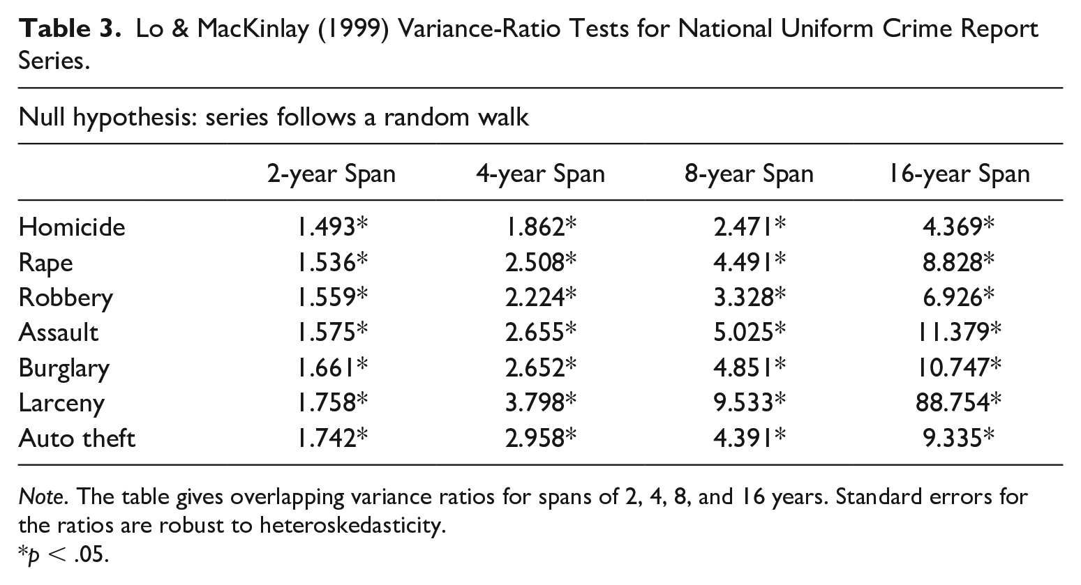
Note. The table gives overlapping variance ratios for spans of 2, 4, 8, and 16 years. Standard errors for the ratios are robust to heteroskedasticity.

p < .05.

Table 4.

ARIMA Models for National Uniform Crime Report Series.

Offense	Model	Coefficient	Estimate	Std. Error
Homicide	(1 − φ₁B) ∇Homicide_t = θ₀ + a_t	φ₁	.2730	.0883*
		θ₀	−.0021	.0109
	Q_22df = 8.693, p = .99
Rape	(1 −φ₁B) ∇Rape_t = θ₀ + a_t	φ₁	.2790	.0937*
		θ₀	.0237	.0096*
	Q_22df = 24.737, p = .31
Robbery	(1 − φ₁B) ∇Robbery_t = θ₀ + a_t	φ₁	.5190	.0886*
		θ₀	−.0104	.0172
	Q_22df = 18.321, p = .6868
Assault	(1 − φ₁B) ∇Assault_t = θ₀ + a_t	φ₁	.4645	.0987*
		θ₀	.0237	.0096*
	Q_22df = 30.386, p = .11
Burglary	(1 − φ₁B) ∇Burglary_t = θ₀ + a_t	φ₁	.6055	.0852*
		θ₀	−.0075	.0159
	Q_22df = 31.445, p = .09
Larceny	(1 − φ₁B – φ₂B) ∇Larceny_t = θ₀ + a_t	φ₁	.7764	.1127*
		φ₂	−.2541	.0911*
		θ₀	.0039	.0125
	Q_22df = 26.521, p = .23
Auto theft	(1 − φ₁B) ∇Auto theft_t = θ₀ + a_t	φ₁	.5615	.0788*
		θ₀	.0006	.0168
	Q_22df = 26.012, p = .25

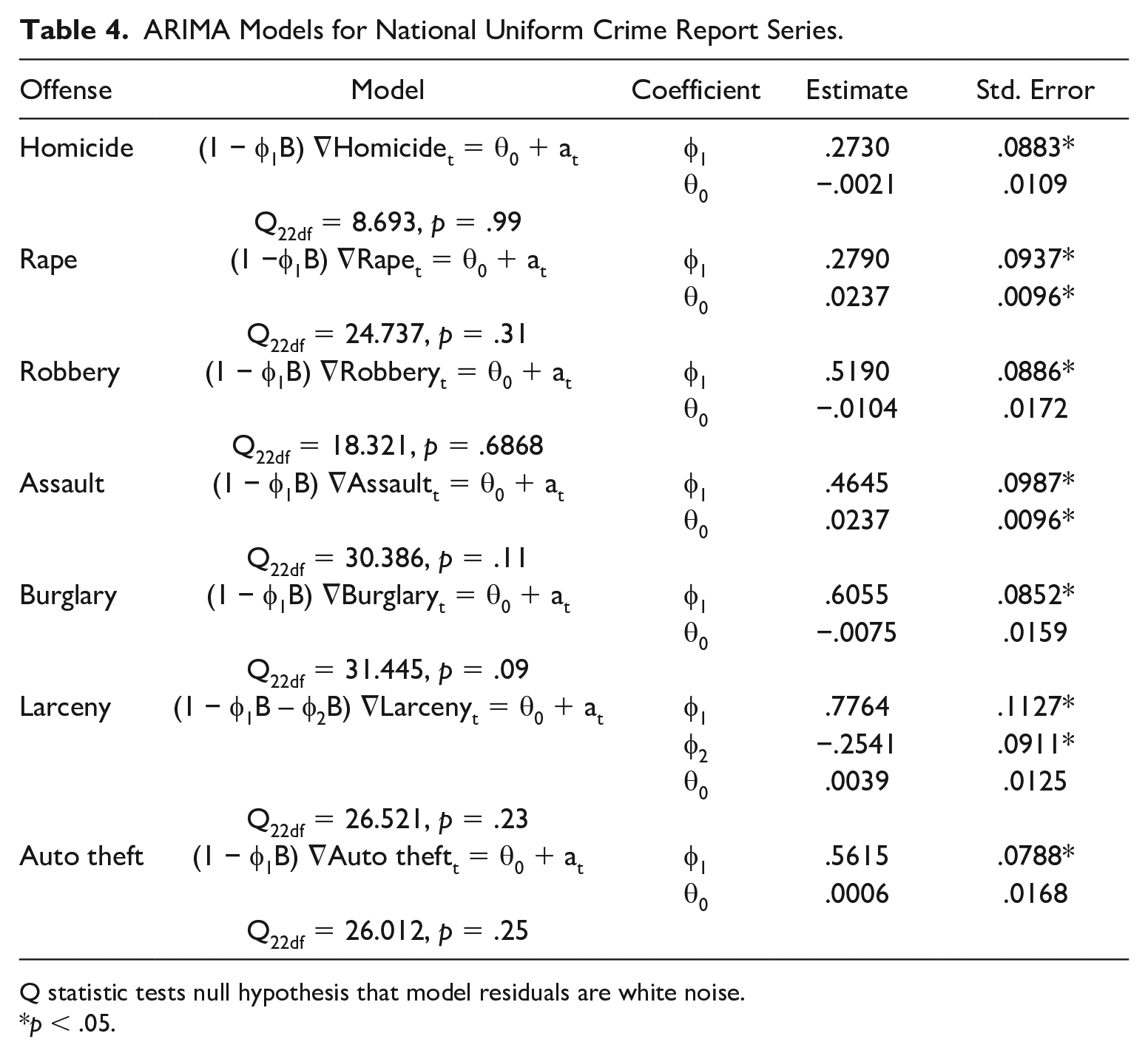
Q statistic tests null hypothesis that model residuals are white noise.

p < .05.

Local homicide rates had a different pattern, with less than half the cities (22 of 47) displaying temporal correlations.³ Like the national series, cities with additional structures were all compatible with autoregressive processes. Unlike the national series, the city autoregressive coefficients were often negative in their signs, with low years followed by high years. As noted previously, this is what one might expect from temporal aggregation.

Although the city trends are more the product of immediate events than the national ones, they are also cross-sectionally correlated. McDowall and Loftin (2005) found that U.S. city crime rate changes displayed considerable correspondence, tending to rise or fall together. They took this similarity as evidence that events at the national level had an impact on local rates.

In the present case, Pesaran’s (2015) CD test for cross-sectional correlations easily rejected the null hypothesis of independence across the city homicide rates. McDowall and Loftin (2005) assessed city-level correspondence using a fixed effects regression model with dummy variables for each year and city. They interpreted the partial correlation for the year dummies as measures of the national influence on city rates. Applying a similar model to the panel cities, the squared partial correlation for the homicide rate changes was .19. Substantively, one can interpret it to mean that national-level events account for about one-fifth of the fluctuation in city rates. Local conditions explain much of the city rate variations, but exogenous national shocks are also influential.

Overall, national crime rates change more smoothly from period-to-period than do the generally random-walking city rates. The form of the changes does not scale from the national level to the local, but both national and city rates are largely due to events over the short term. Large city homicide rates show similar responses to national events, collectively increasing and decreasing with them. Still, with a few exceptions, neither the national nor local rates have equilibrium values, nor do they possess deterministic trends.

Deviations from the Pattern

A model of how crime rates fluctuate allows the study of the existence, size, and timing of deviations from it. Especially for homicide, sudden increases in crime draw significant attention from scholars and policy makers. In recent years, homicide increases in 2005-2006, 2014-2016, and 2020-2021 have received close examination (Rosenfeld & Fox, 2019; Rosenfeld & Lopez, 2022; Rosenfeld & Oliver, 2008).

One approach to understanding a rate increase is to document its scope, studying how it varies over geographical units and demographic groups. Rosenfeld and Fox (2019), for example, apply this strategy to the 2014-2016 homicide increase, locating the categories of victims and circumstances that most contributed to it. The goal is to gain insight into the origin of the increase.

A different approach, and the one that the present paper will use, is to compare rate increases against the pattern of variation over the entire series. Situating an increase within the history of rate changes offers the opportunity to judge its relative extremity, avoiding bump hunting and the temptation to see recent events as unprecedented. Several methods are available for gauging whether departures from a trend are unusual (McDowall, 2019; Wheeler & Kovandzic, 2018). The current article uses perhaps the simplest, which is to check for outlying observations. This analysis considers only the national rate series.

Chen and Liu (1993) distinguish four kinds of outliers, and the analysis will examine the series for evidence of each. Additive outliers are one-time events that produce an unusual change and then disappear. Innovational outliers are unusual events that influence a series for multiple periods through its temporal correlation structure. For autoregressive structures, like those in the national series, the effects of an outlier will linger but eventually die out. Level shifts occur when an outlier permanently moves a series up or down. Finally, transients are temporary level shifts, where a series increases or decreases for a time before settling back to its original level.

Outliers can affect the structure of a time series, and they can hide other outliers. To avoid these possibilities, the analysis uses Chen and Liu’s (1993) method of outlier detection. This involves finding an outlier in a model’s residuals, adjusting the series for it, estimating the model again, and iterating until no other outliers appear. Table 5 reports the results.

Table 5.

Chen and Liu (1993) Analysis of Outliers from Model Estimates in National Uniform Crime Report Series.

Years of occurrence and type for observations more than 2.5 standard errors from their predicted values
Offense	Year	Size	Type	Offense	Year	Size	Type
Homicide	1943	−.149	Level shift	Burglary	1942	−.104	Transient
	1946	.177	Transient		1945	.129	Level shift
	1958	.184	Level shift		1955	−.124	Level shift
	2020	.284	Level shift		1959	−.102	Additive
					1972	−.076	Transient
Rape	1939	.230	Level shift		1974	.099	Level shift
(1930–2019)	1943	.150	Level shift		1980	.083	Transient
	1954	−.103	Additive
	1964	.169	Innovational	Larceny	1972	−.098	Transient
	1969	.065	Additive	(1960−2021)	1974	.156	Innovational
					1976	−.071	Innovational
Robbery	1945	.235	Innovational		1977	−.124	Level shift
	1949	.095	Additive
	1955	−.184	Level shift		1978	−.044	Additive
	1959	−.135	Additive		1985	−.081	Innovational
	1967	.174	Innovational	Auto theft	1942	−.189	Transient
	2000	−.170	Innovational		1946	−.228	Innovational
					1947	−.146	Innovational
Assault	1939	.034	Additive
	1943	−.120	Transient
	1951	−.066	Additive
	1960	.029	Additive
	1964	.095	Level shift
	1976	−.054	Level shift
	1981	−.072	Innovational
	1983	−.047	Transient
	1986	.090	Transient
	1990	.062	Level shift
	1996	−.028	Additive
	2012	.038	Additive
	2020	.116	Transient

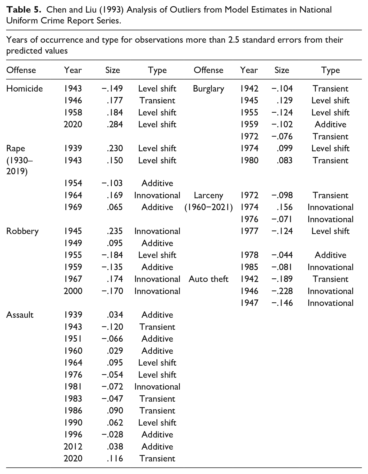
Perhaps the major finding of the analysis is that outliers are infrequent. A conventional definition of an extremely outlying case is one that differs by more than three standard errors from its predicted value (e.g., Box et al., 2008). To produce enough outliers for discussion, the current analysis used a more liberal 2.5 standard errors. Under this definition, only four outliers appear in the homicide rate. Two are a downward level shift in 1943, near the start of World War II, and a transit increase in 1946, after the war ended. The changes in homicides around World War II have been the subject of prior comment (Archer & Gartner, 1984). The third outlier is an upward level shift in 1958, when the FBI changed data collection procedures. This of course hints at deficiencies in the attempt to make the pre- and post-1958 series segments comparable.

The final homicide outlier, and by far the largest, is the increase in 2020. The analysis identifies this as a level shift, presumably because 2021 is also high. As a practical matter, however, not enough time has elapsed since 2020 to be confident in a determination. Although the 2020 and 2021 increases are extreme, they might appear as innovational outliers or as a transient in a longer perspective. It is worth noting that neither the 2005-2006 nor the 2014-2016 homicide increases were large enough for the analysis to flag them as outliers.⁴

The other offenses are like homicide in their infrequency of outliers, and except assault, none had more than seven over the 89-year study period. Outliers occur in several crimes around the time of World War II, but apart from 2020, their timings do not otherwise have much in common.

Besides homicide, assault and robbery also experienced outliers in 2020; assault increased, and robbery decreased. As the series are log-transformed, estimates of the changes are on an approximate percentage scale. The 2020 homicide increase was the largest outlier for any crime in any year during the study period, about 28% above its expected value. Chen and Liu’s methodology labels the assault outlier as a transient and the robbery outlier as innovational, but as with homicide, more time must elapse to categorize them reliably.

Overall, the national rate series display few large deviations from a constant process, even with a generous definition of “large.” Outliers are only one way to discover unusual periods, and other methods could reach different conclusions. Also, city trends should be susceptible to local and state policy changes, and so might display outliers more often. Still, the results here suggest that national crime rates rarely stray far from their generating process.

Nonlinear Mechanisms as an Alternate Explanation

The current paper has assumed that crime-generating processes are constant and linear. Trends in the series are consistent with these features, but other, very different processes might also account for them. Due to space limitations, the article will examine only one possibility, nonlinear generating mechanisms. With a nonlinear process, the size of increases and decreases in a series will depend on whether the series is high or low. This opens the possibility that crime trends are more interesting, and more mysterious, than linear processes allow.

Several plausible mechanisms could generate nonlinear dynamics in crime rates. The most frequently considered of these is contagious transmission (e.g., Cork, 1999; Gladwell, 2000; Loftin, 1986). Here rates can increase or decrease dramatically once they reach a value that serves as a tipping point. Besides contagion, a variety of other reasonable possibilities can also generate the type of rapid growth or decline that nonlinear processes produce (LaFree, 1999).

McDowall (2002) applied multiple tests to evaluate possible nonlinearity in U.S. homicide trends. The results were almost entirely negative, supporting the idea that the rates vary linearly. The logic of nonlinear trends is intuitively appealing, however, and it encourages speculation that they must exist simply because nonlinearity is frequent in nature (Gordon, 2010). Additional investigations are thus desirable, for more crimes and a longer period than McDowall considered.

Nonlinearity includes many specific processes. Although tests can cover multiple possibilities, their power declines as their range expands (Tsay, 1991). Tsay proposed two tests–the TAR-F test and the New-F test–that have high power while still encompassing many types of nonlinearity. Both tests are especially sensitive to threshold autoregressive (TAR) processes.

A TAR model links two or more linear autoregressive models, each with different coefficients. Which model applies at a given moment depends on whether an earlier series value exceeds a threshold. This allows the series to switch back and forth between regimes. A series might increase rapidly if its previous value is above the threshold but decrease slowly if the previous value is below it. TAR models are simple and allow a good variety of nonlinear patterns.

Table 6 presents the results of Tsay tests applied to the national rates. The tests require a decision about how many lagged values should set the threshold, and the analysis considered up to five. For all series, the results did not differ with the choice, and the table therefore reports results for one lag and two regimes. The null hypotheses are thus that a single model provides a better fit to the data than a pair of models.

Table 6.

Nonlinearity Tests for National Uniform Crime Report Series.

Tsay (1991) nonlinearity tests, one threshold lag, two regimes
Null hypothesis: single regime fits entire series
Offense	TAR-F	New-F
Homicide	0.8486, p = .43	0.7966, p = .59
Rape (1930–2019)	3.3976, p = .04	3.8453, p < .01
Robbery	1.7564, p = .18	0.9079, p = .50
Assault	7.2485, p < .01	3.0390, p < .01
Burglary	1.0373, p = .36	1.6719, p = .13
Larceny (1960–2021)	1.5123, p = .22	1.0807, p = .40
Auto theft	0.3166, p = .73	1.9150, p = .08

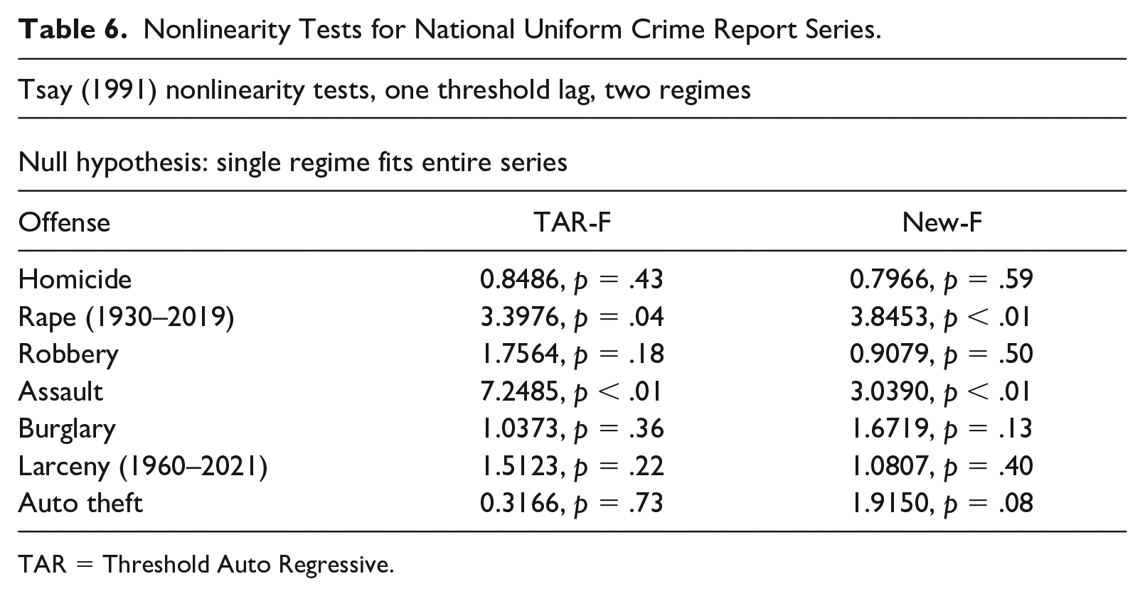
TAR = Threshold Auto Regressive.

Except for rape and assault, the tests yield no evidence of nonlinearity. Rape and assault reject a single model, consistent with nonlinear mechanisms. This possibility is nevertheless open to doubt. In TAR model estimates for the two crimes (not shown here), the only statistically significant regime differences were in the intercept terms. This may result from low power in estimating the models but strictly it means that the nonlinearity finding is due only to linear level shifts.⁵

One other nonlinear possibility deserves a comment. Some observers suggest that homicide rates follow long-period cycles (e.g., Fagan, 2006; Hemenway, 2004; Zimring, 2007). These wavelike variations entail a form of nonlinearity similar to epidemics, and in theory Tsay tests should detect them. The length of the series nevertheless limits the chances of discovering a long cycle statistically. Any evidence for a cycle then comes from the appearance of the series, which arguably shows one (see Figure 1). Random walks can increase and decrease for long periods, however, creating deceptive waves that disappear after differencing. The apparent homicide wave also disappears after differencing, strongly suggesting that it is an artifact of the generating process.

Overall, the analysis does not offer much encouragement for nonlinear mechanisms. Although the series is not entirely incompatible with nonlinearity, evidence in its favor is limited. Tsay tests do reject linearity for two crimes, and the tests do not cover all nonlinear possibilities. Still, based on the findings, linear processes appear adequate to account for the national trends.

Discussion and Conclusion

This article has considered the properties of U.S. crime rate trends and the processes that generate them. The test results are not entirely in agreement, as one might expect from noisy data, but the analysis yields a broadly consistent picture. Measured at annual frequencies, crime rates are not stationarity, either nationally or in large cities. They instead follow random walks or smoothed versions of them, rising and falling with events that occur closely coincident in time. At the national level, the processes appear to have experienced a few large deviations over almost 90 years.

In a sense, the time series processes that appear to underlie crime trends are uninteresting, perhaps even disappointing. For these processes, the past yields few clues to the future, and it offers no exciting insights. The autoregressive components in the national rates can generate relatively accurate short-term forecasts, but their predictive value soon wears off. City rates respond similarly to external shocks and allow the study of national impacts on local trends. By themselves, however, the processes that underlie most city rates do not provide useful predictions.

Simply, the series lack the complicated dynamics that would make their changes interesting in themselves. They do not revert to means and they do not often deviate from their generating processes. They do not follow epidemic curves, and for the most part, they have no attraction to equilibrium values. Instead, they increase and decrease for long periods without bounds, depending on the vagaries of their environment.

In another sense, however, the findings are encouraging in their support for the assumptions of most trend studies. These studies assume linear generating processes, which they try to disaggregate into the influences of individual variables. The studies usually ignore the time series properties of the data that they analyze, possibly compromising their inferences. Even so, their intuition of how rates change is generally in accord with how the processes operate.

Documenting the empirical properties of crime rate trends has implications for criminological research more broadly. The characteristics that the article considers are essentially “stylized facts” about the trends. According to Kaldor (1961; Hirschman, 2016), stylized facts are empirical regularities that capture features of a phenomenon while glossing over the details. In the present case, some large city homicide rates did not reject stationarity, and a claim that homicides follow a nonstationary process is not completely true. Overall, however, the statement generally appears to characterize city trends. Similar considerations apply to other of the paper’s findings.

Stylized facts have been helpful in advancing many substantive areas, especially in economics. Hirschman (2016) suggests three possible reactions to a proposed stylized fact. First, scholars may accept it and attempt to explain it with existing or new theories. Second, scholars may reject it, showing why it is incorrect. Third, scholars may propose ways to extend it or revise it. Importantly, all these reactions help direct and advance research on the topic under study.

This article has considered only a few questions about crime trends from which stylized facts may emerge. Other possibilities include structural changes in the rate generating process (see, e.g., McDowall & Loftin, 2005), rate volatility, fractional nonstationarity, and scaling at various levels of aggregation. The analysis found that the generating structures of crime trends differ somewhat at the national and city levels. Trends could also differ at other levels of aggregation, such as neighborhoods and micro places. The current study has in addition examined rates only at annual frequencies, and monthly, weekly, daily, and intra-daily fluctuations may present other stylized facts. Monthly rates display seasonal variations, for example, and these have their own unique properties (see, e.g., McDowall & Curtis, 2015).

The empirical orientation of the paper is of course prone to various limitations. Data-based conclusions rest on statistical tests, and these are necessarily vulnerable to error. Multiple tests exist for some features, and different tests can lead to different conclusions. Accuracy aside, time goes on and the “facts” of an earlier period may disappear over a longer time scale.

At the broadest level, this paper’s goal was to call attention to the processes that underlie crime trends and to encourage the study of their features. Although now not widely used, investigating the properties of a series is helpful for understanding its fluctuations and for developing and testing theories. As such, it fits well with the Baumer et al. (2018) call for a systematic program of crime trend research. Future uses of the approach should be helpful for expanding the current paper’s claims, and for challenging them.

Supplemental Material

sj-docx-1-ccj-10.1177_10439862231189979 – Supplemental material for Empirical Properties of Crime Rate Trends

Supplemental material, sj-docx-1-ccj-10.1177_10439862231189979 for Empirical Properties of Crime Rate Trends by David McDowall in Journal of Contemporary Criminal Justice

Footnotes

Declaration of Conflicting Interests

The author(s) declared no potential conflicts of interest with respect to the research, authorship, and/or publication of this article.

Funding

The author(s) received no financial support for the research, authorship, and/or publication of this article.

Supplemental Material

Supplemental material for this article is available online.

Notes

Author Biography

David McDowall is a professor in the School of Criminal Justice at the University at Albany-SUNY and co-director of the Violence Research Group. His research interests include crime trends in the United States and the world and the social distribution and consequences of criminal victimization. His most recent book, with coauthors Richard McCleary and Bradly J. Bartos, is Interrupted Time Series Analysis (Oxford University Press, 2019).

References

Archer

Gartner

(1984). Violence and crime in cross-national perspective. Yale University Press.

Baumer

E. P.

Vélez

M. B.

Rosenfeld

(2018). Bringing crime trends back into criminology: A critical assessment of the literature and a blueprint for future inquiry. Annual Review of Criminology, 1, 39–61.

Baumer

E. P.

Wolff

K. T.

(2014). Evaluating contemporary crime drop(s) in America, New York City, and many other places. Justice Quarterly, 31, 5–38.

Blumstein

Wallman

(Eds.). (2007). The crime drop in America. Cambridge University Press.

Box

G. E. P.

Jenkins

G. M.

Reinsel

G. C.

(2008). Times series analysis: Forecasting and control (4th ed.). Wiley.

Chen

Liu

L.-M.

(1993). Joint estimation of model parameters and outlier effects in time series. Journal of the American Statistical Association, 88, 284–297.

Cork

(1999). Examining space-time interaction in city-level homicide data: Crack markets and the diffusion of guns among youth. Journal of Quantitative Criminology, 15, 379–406.

Durkheim

(1966). The rules of sociological method. Free Press. (Original work published 1895).

Enders

(2015). Applied econometric time series (4th ed.). Wiley.

10.

Fagan

(2006). Death and deterrence redux: Science, law, and causal reasoning on capital punishment. Ohio State Journal of Criminal Law, 4, 255–320.

11.

Friedman

Hakim

Spiegel

(1989). The difference between short and long run effects of police outlays on crime. American Journal of Economics and Sociology, 48, 177–191.

12.

Gladwell

(2000). The tipping point: How little things can make a big difference. Little, Brown.

13.

Gordon

M. B.

(2010). A random walk in the literature on criminality: A partial and critical view on some statistical analyses and modelling approaches. European Journal of Applied Mathematics, 21, 283–306.

14.

Greenberg

D. F.

(2001). Time series analysis of crime rates. Journal of Quantitative Criminology, 17, 291–327.

15.

Harcourt

B. E.

Ludwig

(2016). Broken windows: New evidence from New York City and a five-city social experiment. University of Chicago Law Review, 73, 271–320.

16.

Hemenway

(2004). Private guns, public health. University of Michigan Press.

17.

Hirschman

(2016). Stylized facts in the social sciences. Sociological Science, 3, 604–626.

18.

Kaldor

(1961). Capital accumulation and economic growth. In Hague

D. C.

(Ed.), The theory of capital (pp. 177–222). Palgrave Macmillan.

19.

Kovandzic

T. V.

Vertatis

L. M.

Boots

D. P.

(2009). Does the death penalty save lives? New evidence from state panel data, 1977 to 2006. Criminology & Public Policy, 8, 803–841.

20.

LaFree

(1999). Declining violent crime rates in the 1990’s: Predicting crime booms and busts. Annual Review of Sociology, 25, 145–168.

21.

Lauritsen

Rezey

Heimer

(2016). When choice of data matters: Analyses of U.S. crime trends, 1973–2012. Journal of Quantitative Criminology, 32, 335–355.

22.

A. W.

MacKinlay

A. C.

(1999). A non-random walk down Wall Street. Princeton University Press.

23.

Loftin

(1986). Assaultive violence as a contagious social process. Bulletin of the New York Academy of Medicine, 62, 550–555.

24.

Maddala

G. S.

Kim

I.-M.

(1998). Unit roots, cointegration, and structural change. Cambridge University Press.

25.

McDowall

(2002). Tests of nonlinear dynamics in U.S. homicide time series, and their implications. Criminology, 40, 711–735.

26.

McDowall

(2019). The 2015 and 2016 U.S. homicide rate increases in context. Homicide Studies, 23, 225–242.

27.

McDowall

Curtis

(2015). Seasonal variation in homicide and assault across large U.S. cities. Homicide Studies, 19, 303–325.

28.

McDowall

Loftin

(2005). Are U.S. crime rate trends historically contingent? Journal of Research in Crime and Delinquency, 42, 359–383.

29.

Messner

S. F.

Rosenfeld

(2013). Crime and the American dream (5th ed.). Wadsworth.

30.

Narayan

P. K.

Nielsen

Smyth

(2010). Is there a natural rate of crime? American Journal of Economics and Sociology, 69, 759–782.

31.

Pesaran

M. H.

(2012). On the interpretation of panel unit root tests. Economics Letters, 116, 545–546.

32.

Pesaran

M. H.

(2015). Time series and panel data econometrics. Oxford University Press.

33.

Philipson

T. J.

Posner

R. A.

(1996). The economic epidemiology of crime. Journal of Law and Economics, 39, 405–433.

34.

Rosenfeld

(2007). Explaining the divergence between UCR and NCVS aggravated assault trends. In Lynch

J. P.

Addington

L. A.

(Eds.), Understanding crime statistics: Revisiting the divergence of the NCVS and the UCR (pp. 251–268). Cambridge University Press.

35.

Rosenfeld

Fox

J. A.

(2019). Anatomy of the homicide rise. Homicide Studies, 23, 202–224.

36.

Rosenfeld

Lopez

(2022). Pandemic, social unrest, and crime in U.S. Cities: Year-end 2021update. Council on Criminal Justice.

37.

Rosenfeld

Messner

S. F.

(2010). The normal crime rate, the economy, and mass incarceration: An institutional anomie perspective on crime control policy. In Barlow

H. D.

Decker

S. H.

(Eds.), Criminology and public policy: Putting theory to work (pp. 45–65). Temple University Press.

38.

Rosenfeld

Oliver

(2008). Evaluating recent changes in homicide and robbery rates. Justice Research and Policy, 10, 49–65.

39.

Tsay

(1991). Detecting and modelling nonlinearity in univariate time series analysis. Statistica Sinica, 14, 31–51.

40.

U.S. Office of Management and the Budget. (1973). Social indicators, 1973: Selected statistics on social conditions and trends in the United States. Office of Management and Budget, Statistical Policy Division.

41.

Wheeler

A. P.

Kovandzic

T. V.

(2018). Monitoring volatile homicide trends across U.S. cities. Homicide Studies, 22, 119–144.

42.

Witt

Witte

(2000). Crime, prison, and female labor supply. Journal of Quantitative Criminology, 16, 69–85.

43.

Zimring

F. E.

(2007). The great American crime decline. Oxford University Press.

Supplementary Material

Please find the following supplemental material available below.

For Open Access articles published under a Creative Commons License, all supplemental material carries the same license as the article it is associated with.

For non-Open Access articles published, all supplemental material carries a non-exclusive license, and permission requests for re-use of supplemental material or any part of supplemental material shall be sent directly to the copyright owner as specified in the copyright notice associated with the article.

0.00 MB

0.04 MB