
Abstract
The likelihood that a study will yield statistically significant results depends on the chosen sample size. Surveillance and diagnostic situations that require sample size calculations include certification of disease freedom, estimation of diagnostic accuracy, comparison of diagnostic accuracy, and determining equivalency of test accuracy. Reasons for inadequately sized studies that do not achieve statistical significance include failure to perform sample size calculations, selecting sample size based on convenience, insufficient funding for the study, and inefficient utilization of available funding. Sample sizes are directly dependent on the assumptions used for their calculation. Investigators must first specify the likely values of the parameters that they wish to estimate as their best guess prior to study initiation. They further need to define the desired precision of the estimate and allowable error levels. Type I (alpha) and type II (beta) errors are the errors associated with rejection of the null hypothesis when it is true and the nonrejection of the null hypothesis when it is false (a specific alternative hypothesis is true), respectively. Calculated sample sizes should be increased by the number of animals that are expected to be lost over the course of the study. Free software routines are available to calculate the necessary sample sizes for many surveillance and diagnostic situations. The objectives of the present article are to briefly discuss the statistical theory behind sample size calculations and provide practical tools and instruction for their calculation.
Introduction
Calculation of sample size is important for the design of epidemiologic studies, 18,62 and specifically for surveillance 9 and diagnostic test evaluations. 6,22,32 The probability that a completed study will yield statistically significant results depends on the choice of sample size assumptions and the statistical model used to make calculations. The statistical methodology of employed sample size calculations should parallel the proposed data analysis to the extent possible. 18 The most frequently chosen sample size routines are based on frequentist statistics, and these have been reviewed previously for other fields. 1,11,20,33,35,36,50,54,61,10 Issues specifically related to diagnostic test validation also have been discussed. 2,28,42,48 Sample size routines related to issues of surveillance, as well as diagnostic test validation using Bayesian methodology, also have been developed. 7,56
Surveillance and diagnostic situations that require sample size calculations include the detection of disease in a population to certify disease freedom, estimation of diagnostic accuracy, comparison of diagnostic accuracy among competing assays, and equivalency testing of assays. The appropriate sample size depends on the study purpose, and no calculations can be made until study objectives have been defined clearly. Sample size calculations are important because they require investigators to clearly define the expected outcome of investigations, encourage development of recruitment goals and a budget, and discourage the implementation of small, inconclusive studies. Common sample size mistakes include not performing any calculations, making unrealistic assumptions, failing to account for potential losses during the study, and failing to investigate sample sizes over a range of assumptions. Reasons for inadequately sized studies that do not achieve statistical significance include failing to perform sample size calculations, selecting sample size based on convenience, failing to secure sufficient funding for the project, and not using available funding efficiently.
There is no single correct sample size “answer” for any given epidemiologic study objective or biologic question. Calculated sizes depend on assumptions made during their calculation, and such assumptions cannot be known with certainty. If assumptions were known to be true with certainty, then the study that is being designed will likely not add to the scientific understanding of the problem. There are concepts that are important to consider when performing sample size calculations, despite the inability to classify certain results as correct or incorrect. A few simple formulas are generally sufficient for most sample size situations that would be encountered in the design of studies to determine disease freedom and evaluate diagnostic tests. The objectives of the present article are to briefly discuss the statistical theory behind sample size calculations and provide practical tools and instruction for their calculation. This review will only discuss issues related to frequentist approaches to sample size calculation and will emphasize conservative methods that result in larger sample sizes.
Definition of type I and type II errors.*
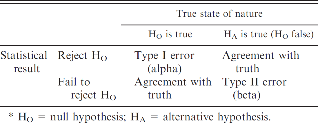
HO = null hypothesis; HA = alternative hypothesis.
Epidemiologic errors
The current presentation of statistical results in the medical literature tends to be a blending of significance testing attributed to the work of Fisher, 21 subsequently discussed by others, 29,55 and hypothesis testing as attributed to Neyman and Pearson. 46,47 The P value in the Fisher significance testing approach is considered a quantitative value documenting the level of evidence for or against the null hypothesis. The P value is formally defined as the probability of observing the current data or more extreme when the null hypothesis is true. The hypothesis testing approach as introduced by Neyman and Pearson was based on rejection or acceptance of null hypotheses using specified P value cutoffs. The hypothesis testing interpretation of statistical results allows for the definition of type I and type II errors as the errors associated with rejection of the null hypothesis when it is indeed true and the acceptance of the null hypothesis when it is false (and a particular alternative hypothesis is true), respectively. 47 The probabilities of making these errors are frequently referred to as alpha (α) and beta (β) for type I and type II errors, respectively. 36,54 Current sample size procedures are derived from the hypothesis testing approach as put forth by Neyman and Pearson; however, current convention is to use the terminology of “failure to reject” rather than acceptance of a null hypothesis.
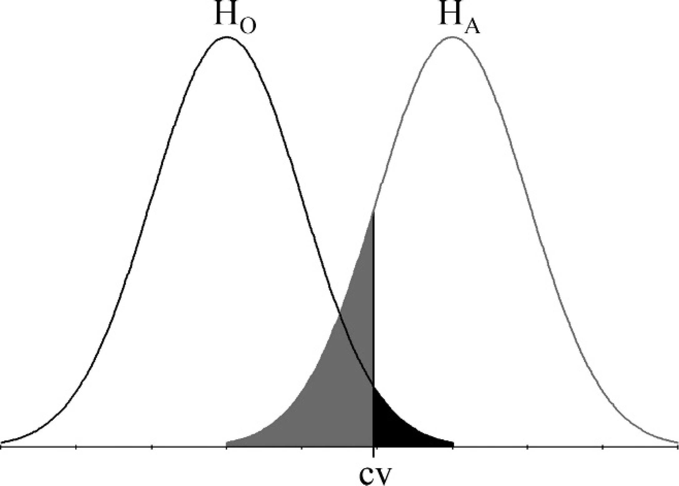
Sampling distributions presented under the null (HO, black line) and alternative (HA, gray line) hypotheses. Black shaded area corresponds to alpha (type I error), and gray shaded area corresponds to beta (type II error). Sample size calculations solve for the number so that the critical value (cv) corresponds to the location, where Pr Z ≤ z = 1 – α/2 and Pr Z ≤ z = β (or Pr Z ≤ z = 1 – α for a 1-sided test).
A requirement for sample size calculation is the specification of alpha and beta when considering the testing of a statistical hypothesis (Table 1). Precision-based sample size methods must specify alpha, but beta is not included in the equations and, based on the typical large-sample approximation methods, is consequently assumed to be 50% for the alternative hypothesis that the true value falls outside the limits of the calculated confidence interval. 17 The P value obtained after statistical analysis will equal the prespecified alpha if the assumptions of the sample size calculations are observed exactly in the collected data due to their similar probabilistic definition. However, the meaning of beta is often misunderstood as simply “the probability of accepting the null hypothesis when a true difference exists” based on presentations in tables and figures. 11,33,36,54 The issue is that there are an infinite number of specific alternative hypotheses that could be true if the null hypothesis is false, and many will be less probable than the null itself. Beta can be calculated only after an explicit alternative hypothesis has been specified. The hypothesis that is chosen during sample size calculation is the expected difference between the population values. Alpha and beta correspond to areas under sampling distributions for population means (including proportions) under the null and alternative hypotheses, respectively (Fig. 1). The statistical power of a test is defined as 1 – β or the probability of rejecting the null hypothesis when the alternative hypothesis is true.
Sample size adjustment factors
Sample size calculations are often based on large-sample approximation methods. 24,30,51 The quality of the approximate results depends on the specific sample size situation, and adjustment factors have been developed to improve their approximation to exact distributions. Some of the typical adjustment factors include the finite population, continuity correction, and variance inflation factors.
The finite population correction factor 4,19 is typically considered when the study objective is to estimate a population proportion. Typically, sampling without replacement is performed, and if the sample size is relatively large compared with the total population, then this correction factor should be considered. A typical recommendation is to employ this factor when the sample includes 10% or more of the population. 19 The need for this correction factor is derived from the fact that sampling is hypergeometric (sampling without replacement, as from a deck of cards), and sample size formulas are based on binomial (sampling with replacement) theory. The formula 19 for the correction is
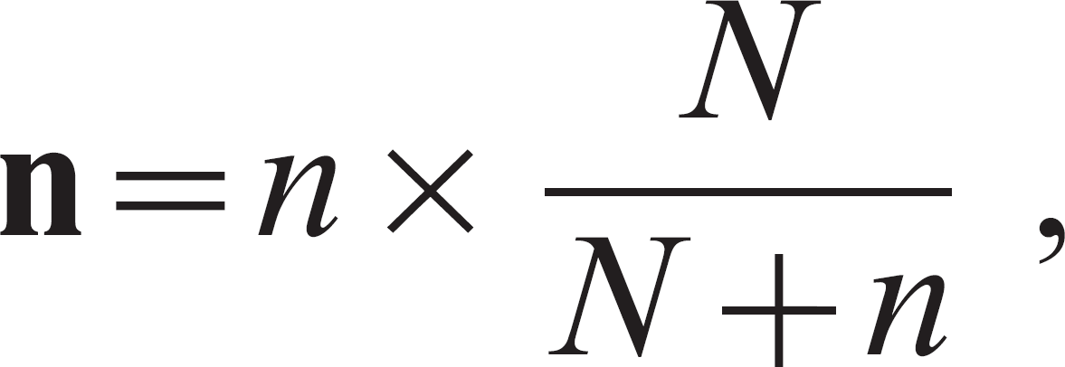
where
The continuity correction factor
51
is employed when the study objective is to compare 2 population
proportions (including diagnostic sensitivity or specificity). The difference in proportions
is approximated by a normal distribution in typical sample size formulas, even though
binomial distributions are discrete and normal distributions are continuous. The normal
approximation might not always be adequate, and continuity correction should be applied to
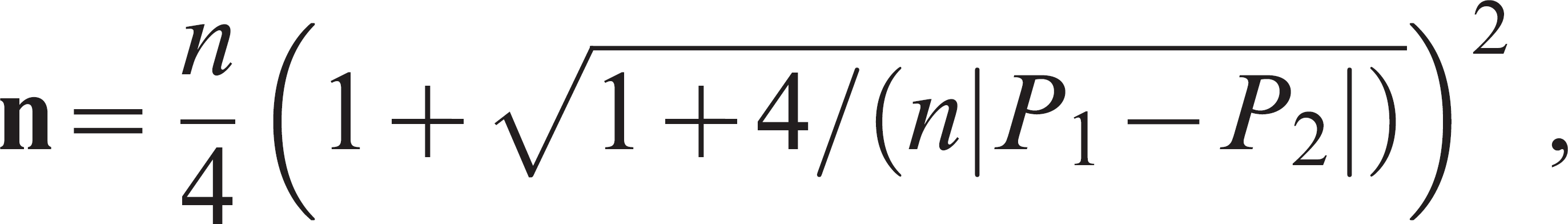
better approximate the exact distribution (Fig. 2). The formula
25
for continuity correction is where
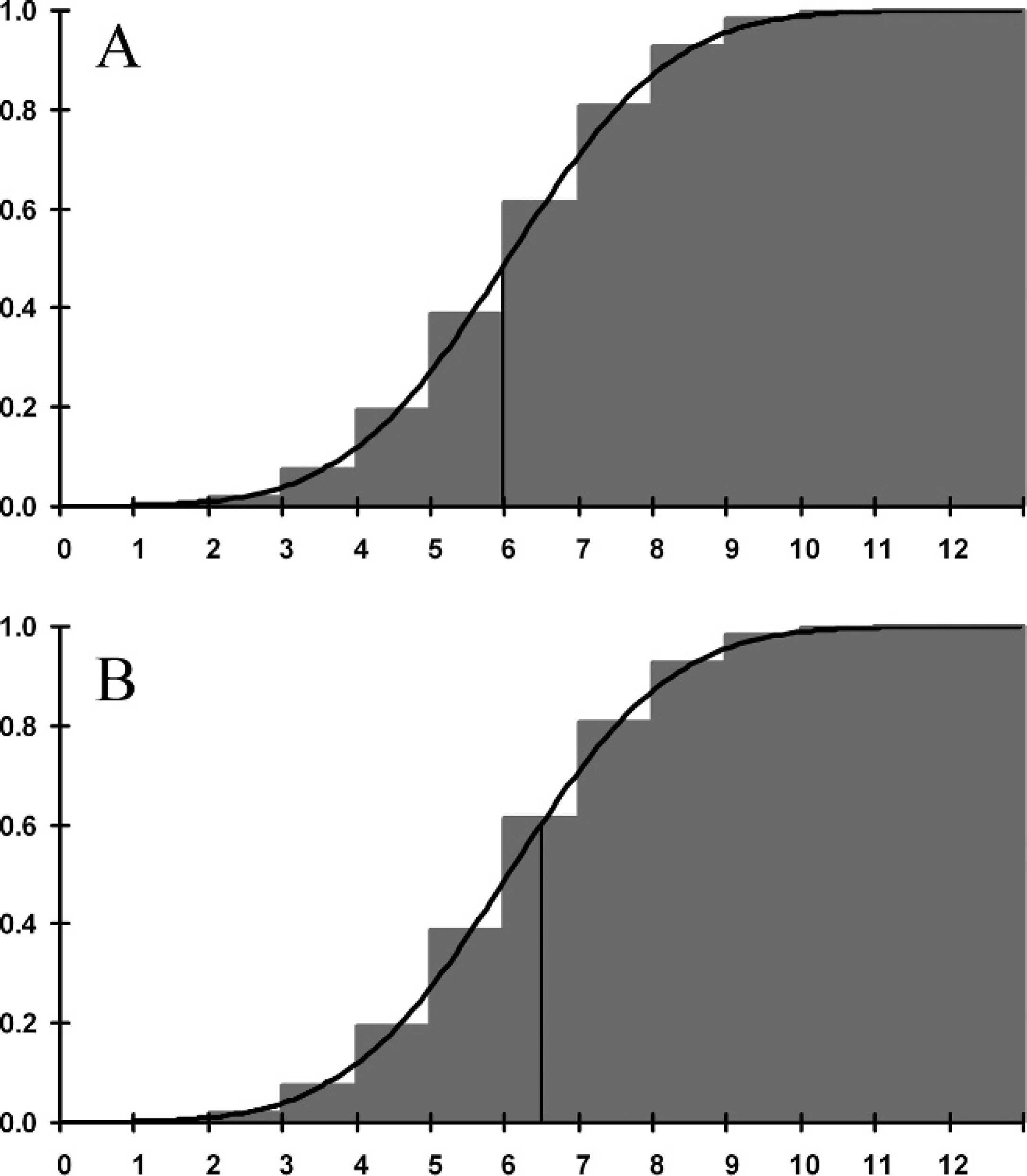
Cumulative probability function for a binomial distribution (n = 12, p = 0.5) (gray
shading) overlaid with the corresponding cumulative normal distribution (μ = 6, σ =
1.732) denoting the uncorrected (
Sample size calculations for estimating proportions typically involve making the assumption of independence among sampling units. Lack of independence that is introduced when a clustered sampling design is employed can be adjusted by inflating the variance estimate. The design effect (DE), 10,38 or variance inflation factor, is defined as the variance of the sampling design compared with simple random sampling. The formula 10,45,59 for its calculation is
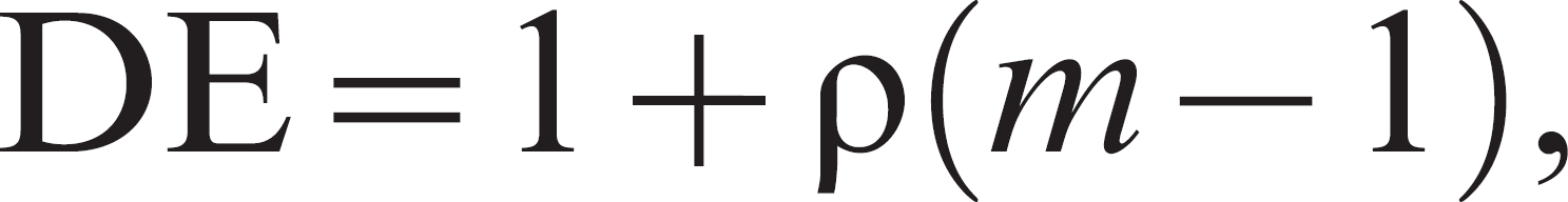
where ρ is the intraclass correlation, and m is the sample size within each cluster. When clustered sampling is employed, then the sample size estimated by the usual methods assuming independence is multiplied by the DE to account for the expected dependence.
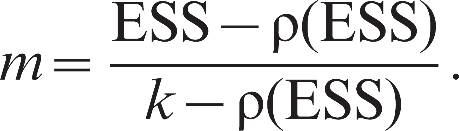
The intraclass correlation is a relative measure of the homogeneity of sampling units within each cluster compared with a randomly selected sampling unit. This correlation is formally defined as the proportion of total variation within sampling units that can be accounted by variation among clusters. 38,45 A high correlation indicates more dependence within the data, resulting in a larger DE. The intraclass correlation is generally estimated from pilot data or based on estimates available from the literature. If the number of clusters is fixed by design and the cluster sample size is unknown, then it is not possible to simply use the previously mentioned formula for the DE. The sample size per cluster (m) must first be estimated, and it is based on the effective sample size (ESS), which is the sample size estimated assuming independence. It is also necessary to know the number of clusters (k) and the intraclass correlation (ρ). The formula 27 for calculation of the cluster sample size is
Sample size situations
Surveillance or detection of disease
The detection of disease in a population is important for herd certification programs and for documenting freedom from disease after an outbreak. It has implications in regional and international trade of animals and animal products. The first step is to determine the prevalence of disease that is important to detect. A prevalence of disease at this level or greater is considered biologically important. Documenting a zero prevalence of disease is not typically possible because it would require testing the entire population with a perfect assay. The next step is to define the level of confidence for which it is desired to find the disease should it be present in the population at the hypothesized prevalence or higher. Again, 100% confidence is not feasible because it would require sampling all animals and testing with a perfect assay. Alpha is calculated as 1 – confidence. The final step is to determine the statistical model to use for calculations. In small populations, sample size calculations should be based on a hypergeometric distribution (sampling without replacement). In larger populations, it is often assumed that the true hypergeometric distribution can be well approximated by the binomial (sampling with replacement). The sample size formula assuming a binomial model is based on the following relationship: (1 – p) n = (1 – confidence). The formula 19 after solving for the sample size is
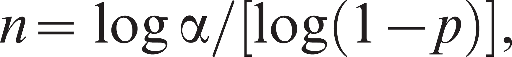
where α is 1 – confidence, and p is the prevalence worth detecting. The corresponding formula 19 based on hypergeometric sampling is
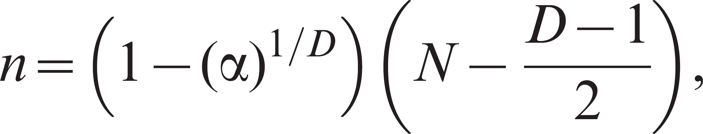
where α is 1 – confidence, N is the population size, and D is the expected number of diseased animals in the population.
The necessary sample size for various combinations of prevalence and confidence can be tabulated (Table 2), and software is available that will perform the necessary calculations. Survey Toolbox a can perform these calculations and is available free for download. The software performs calculations based on both binomial and hypergeometric sampling and can also adjust for imperfect sensitivity and specificity of employed tests.
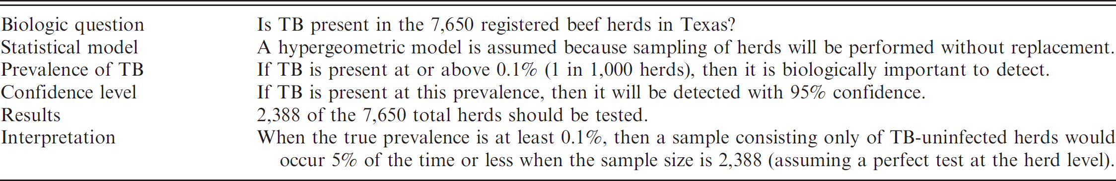
An example of this type of sample size problem is illustrated by the regulatory agency in
Texas when it decided to perform active surveillance for bovine tuberculosis (Table 3). There are approximately
7,650 registered pure-bred beef seed stock producers in Texas, and it was decided that a
herd-level prevalence of 0.001 (1 in 1,000 herds infected) or greater was important to
detect with 95% confidence. Survey Toolbox can be used to solve this sample size problem.
From the menu, choose
A binomial model suggested that the necessary sample size would be 2,994 of the 7,650 beef operations (39%). The interpretation is that assuming that the true prevalence is at least 0.001, then a sample consisting only of noninfected herds would occur 5% of the time or less when the sample size is 2,994 (assuming a perfect test at the herd level). The hypergeometric model might be more appropriate, because sampling would be from a finite population without replacement; using the hypergeometric formula, the sample size is 2,388 herds (31%) of the 7,650 total.
Number needed for study to be confident that the disease will be detected if present at or above a specified prevalence based on hypergeometric sampling and assuming a perfect test.
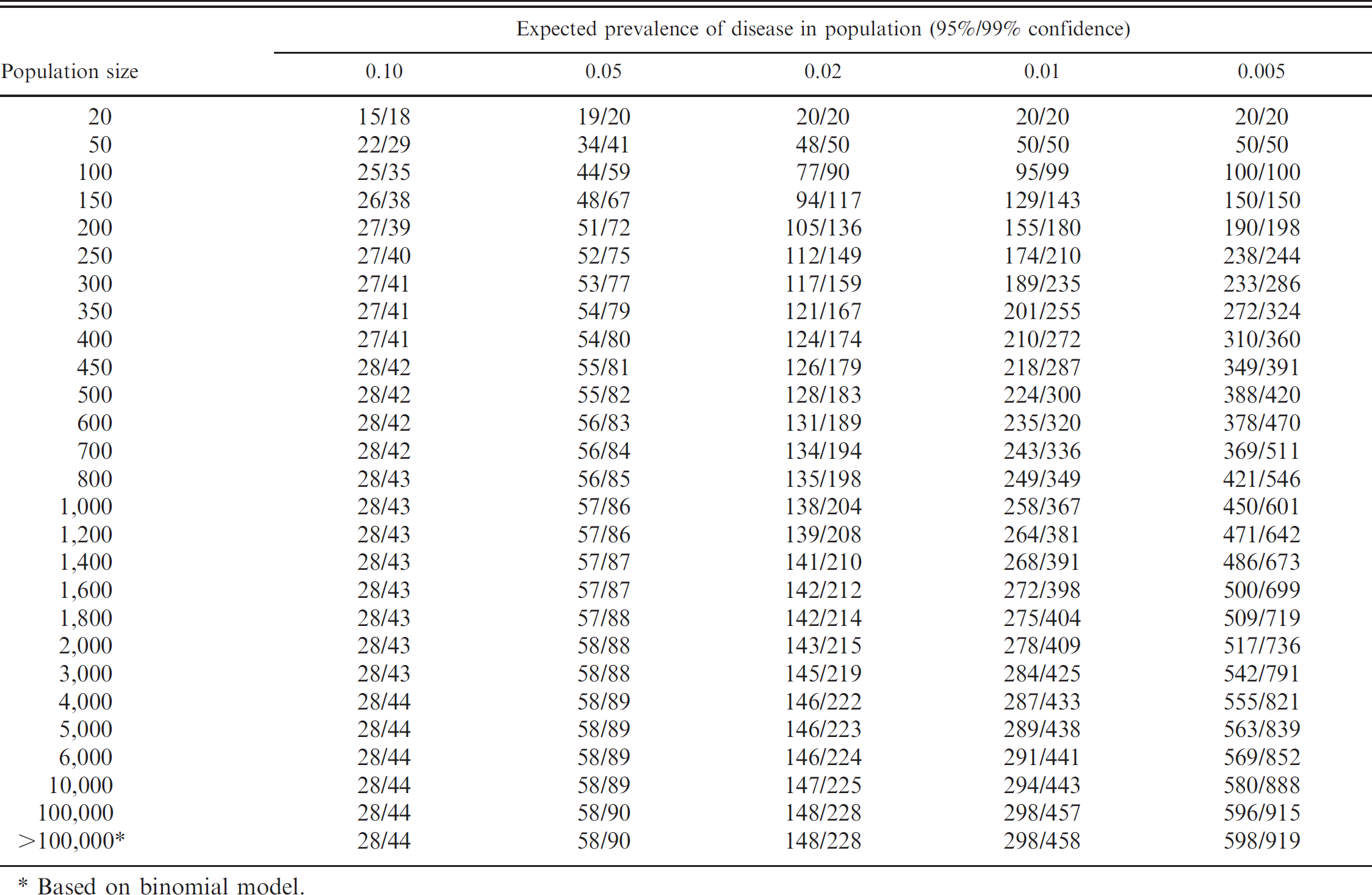
Based on binomial model.
Estimation of a population proportion
Calculating the sample size necessary to estimate a population proportion is important when an estimate of disease prevalence or diagnostic test validation is desired. The sensitivity and specificity of an assay should be considered population estimates in the same manner as other proportions. The sample size formulas employed for these calculations are typically considered to be precision based because they involve finding confidence intervals of a specified width rather than testing hypotheses. The typical sample size formula 37,58 based on the normal approximation to the binomial is
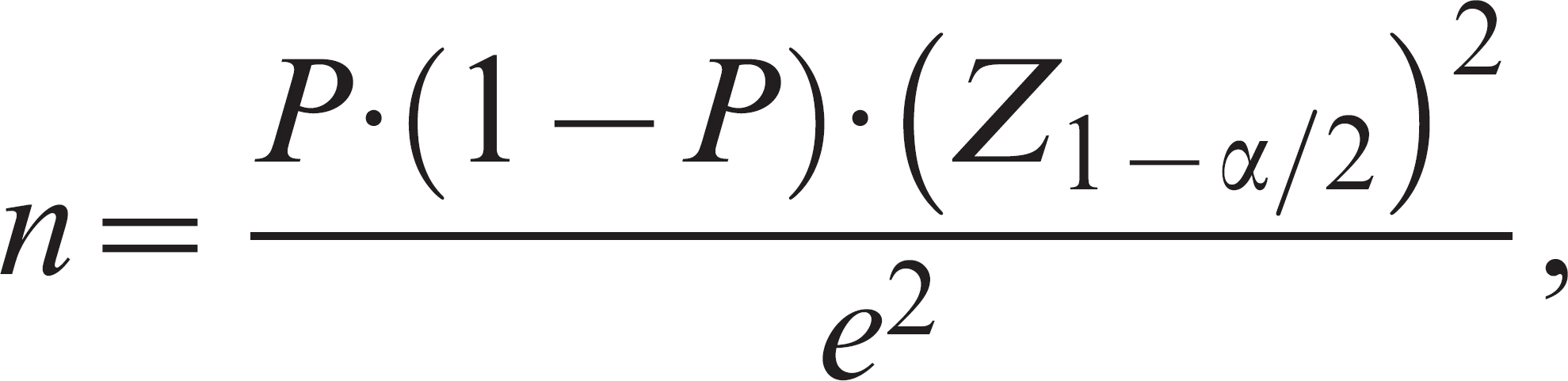
where P is the expected proportion (e.g., diagnostic sensitivity), e is one half the desired width of the confidence interval, and Z1–α/2 is the standard normal Z value corresponding to a cumulative probability of 1 – α/2. The investigator must specify a best guess for the proportion that is expected to be found after performing the study. The investigator also needs to specify the desired width of the interval around this proportion and the level of confidence. In essence, this procedure will find the sample size that, upon statistical analysis, would result in a confidence interval with the specified probability and limits if the assumed proportion were in fact observed by the study (Fig. 3). The resulting sample size could be adjusted using the finite population correction factor, and if this is performed then the statistical analysis should be similarly adjusted at the end of the study. Sample sizes calculated using formulas should always be rounded up to the nearest whole number.
Sample size situation for the detection of bovine tuberculosis (TB) in beef cattle herds.

The sample size is determined so that the sampling distribution of the hypothesized
proportion () has an area under the curve between the specified upper
(PU) and lower (PL) bounds of
the confidence interval equal to the specified probability (grade shaded area);
Pr(PL ≤ ≤
PU) = confidence level.
The sample size methods based on the normal approximation to the binomial might not be adequate when the expected proportion is close to the boundary values of 0 or 1. Exact binomial methods are preferred when the proportion is expected to fall outside the range of 0.2–0.8. 26 The binomial probability function is the basis of exact sample size methods, and it is
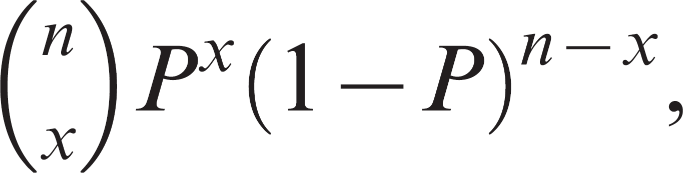
where P is the hypothesized proportion, n is the sample size, and x is the number of observed “successes.”
Derivation of a sample size algorithm based on the binomial probability function has been described previously. 26 It is based on the mid-P adjustment 5,41 for the Clopper-Pearson method of exact confidence interval estimation. 14 The investigator specifies PU and PL as the desired limits of the confidence interval around the hypothesized proportion (P) and the desired level of confidence. The calculated sample size could be adjusted using the finite population correction factor if deemed appropriate.
Software is available to calculate the necessary sample size for estimating population proportions. Epi Info b includes software that can perform these calculations 33 and is available free for download. The software performs calculations based on normal approximation methods and will apply the finite population correction factor if the population size is specified. Software to perform calculations based on binomial exact methods (Mid-P Sample Size routine) can be obtained by contacting the author.
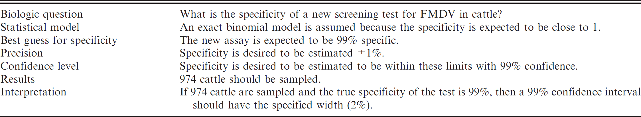
An example of this type of sample size problem is the design of a study to estimate the
diagnostic specificity of a new assay to screen healthy cattle for Foot-and-mouth
disease virus (FMDV; Table
4). The number of cattle necessary to sample could be calculated for an expected
specificity of 0.99 and the desire to estimate this specificity ±0.01 with 99% confidence.
For this example, it will be assumed that sampling is from a large population, and a simple
random sampling design will be employed. Epi Info 6 can be used to make the calculation
based on normal approximation methods (newer versions of Epi Info have not retained
presented sample size routines). From the menu, choose
Sample size situation for estimating the specificity of a test to screen cattle for Foot-and-mouth disease virus (FMDV).
Typically, sample size calculations for studies that will perform clustered sampling first calculate the necessary sample size assuming independence or lack of clustering. Calculated sample sizes are then multiplied by the DE to account for the lack of independence. Expert opinion can be used to account for expected correlation of sampling units when prior information concerning the intraclass correlation is not available. A sample size routine incorporating a method to estimate the DE based on expert opinion for a fixed number of clusters has been developed 27 and is available from the author.
Comparison of 2 proportions
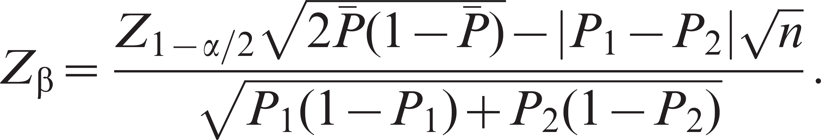
Independent proportions. Calculating the sample size necessary to compare 2 population proportions is important when a comparison of the accuracy of diagnostic tests is desired. Sensitivity and specificity are population estimates, and comparison between 2 assays should be based on this sample size situation. The usual sample size formula 13,25,53 based on the normal approximation to the binomial with equal group sizes is
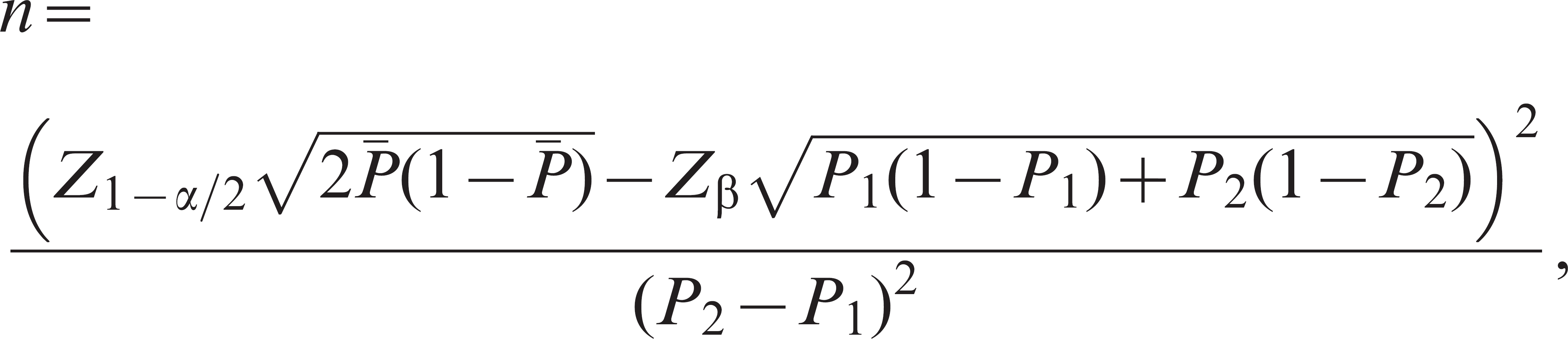
where P1 and P2 are the expected
proportions in each group, and  is the simple
average of the expected proportions. Variables Z1–α/2 and
Zβ are the standard normal Z values
corresponding to the selected alpha (2-sided test) and beta, respectively. Typical
presentation of the formula
11,12
above
uses Zα/2 instead and an addition of the 2 components within the
numerator. Solving these 2 formulations gives the same sample size because the numerator is
squared. The specific formulation has been included here because alternative hypotheses have
been presented in figures as being on the positive side of the null hypothesis, and
therefore Zβ should be negative. This is also consistent with
the algebraic manipulation to solve for Zβ, as presented in the
section related to power calculation. The resulting sample size should be adjusted using the
continuity correction factor, and all sample sizes should be rounded up to the nearest whole
number. The magnitude of the difference between the 2 proportions has a greater effect on
calculated sample sizes than typical values for alpha and beta (Fig. 4). The absolute magnitude of the proportions
affects the calculations, with proportions closer to 0.5 resulting in larger sample
sizes
11
because
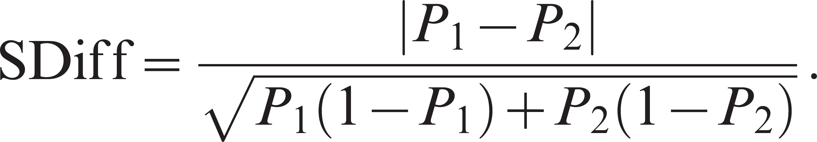
the variance of a proportion is greatest at this value. The formula for the standardized
difference (SDiff) in proportions
3,36,61
is
is the simple
average of the expected proportions. Variables Z1–α/2 and
Zβ are the standard normal Z values
corresponding to the selected alpha (2-sided test) and beta, respectively. Typical
presentation of the formula
11,12
above
uses Zα/2 instead and an addition of the 2 components within the
numerator. Solving these 2 formulations gives the same sample size because the numerator is
squared. The specific formulation has been included here because alternative hypotheses have
been presented in figures as being on the positive side of the null hypothesis, and
therefore Zβ should be negative. This is also consistent with
the algebraic manipulation to solve for Zβ, as presented in the
section related to power calculation. The resulting sample size should be adjusted using the
continuity correction factor, and all sample sizes should be rounded up to the nearest whole
number. The magnitude of the difference between the 2 proportions has a greater effect on
calculated sample sizes than typical values for alpha and beta (Fig. 4). The absolute magnitude of the proportions
affects the calculations, with proportions closer to 0.5 resulting in larger sample
sizes
11
because
the variance of a proportion is greatest at this value. The formula for the standardized
difference (SDiff) in proportions
3,36,61
is
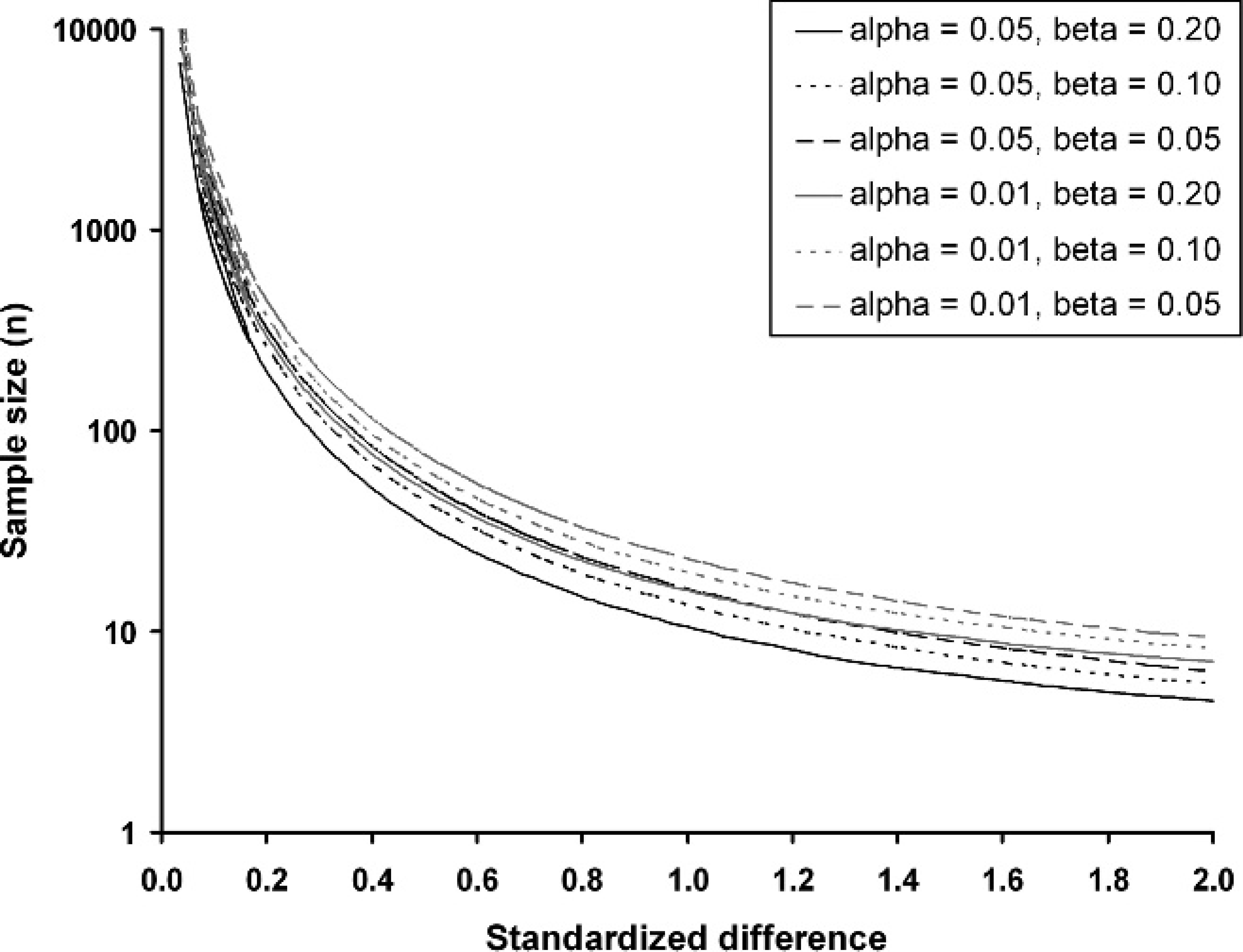
Sample size estimates are affected by the standardized difference and the specified alpha (type I error) and beta (type II error).
Software is available to calculate the necessary sample size to compare 2 independent
population proportions. Epi Info
b
can be used to perform these calculations. The calculations are
based on normal approximation methods and will apply a continuity correction factor. An
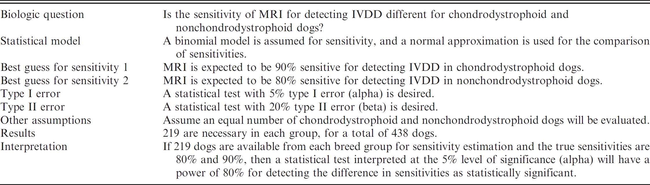
example of this type of sample size problem is the design of a study to compare the
diagnostic sensitivity of magnetic resonance imaging (MRI) for detection of intervertebral
disk disease between chondrodystrophoid and nonchondrodystrophoid breeds of dogs (Table 5). The number of dogs
necessary to sample could be calculated for expected sensitivities of 90% and 80% in
chondrodystrophoid and nonchondrodystrophoid dogs, respectively. The statistical test could
be desired to have an alpha of 5% and beta of 20% to detect this difference in proportions.
The ratio of chondrodystrophoid to nonchondrodystrophoid dogs also needs to be specified,
and the assumption could be made to have equal group sizes. Epi Info 6 can be used to make
the calculation. From the menu, choose
Sample size situation for comparing the sensitivity of magnetic resonance imaging (MRI) for detection of intervertebral disk disease (IVDD) between chondrodystrophoid and nonchondrodystrophoid breeds of dogs.
Sample size calculations for the comparison of proportions when the group sizes are not equal are a simple modification of the presented formula. 60 The formula also can be modified to allow for the estimation of odds ratios and risk ratios. 20,53 All presented formulas correspond to the necessary sample sizes for 2-sided statistical tests. Variable Z1–α/2 is replaced with Z1–α to modify the formula for a 1-sided test.
Dependent proportions. When multiple tests are performed based on
specimens collected from the same animal, then the proportions (i.e., sensitivity and
specificity) should be considered dependent. There are multiple conditional and
unconditional approaches to solving this sample size problem,
15,16,23,39,40,43,44,49,57
and a formula is not presented in this
section due to increased complexity and lack of consensus among competing methods. An
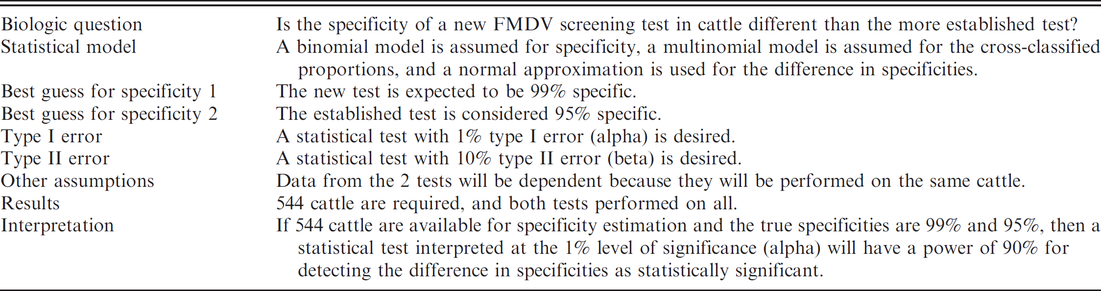
example of this type of sample size problem is the design of a study to compare the
diagnostic specificity of 2 tests for FMDV screening in healthy cattle (Table 6). Serum samples from each
selected animal for study will have both tests performed in parallel. The number of cattle
necessary to sample could be calculated based on expected specificities of 99% and 95% in
test 1 and test 2, respectively. The statistical test could be desired to have alpha be 1 %
and beta 10% to detect this difference in proportions. Software is available to calculate
the necessary sample size to compare 2 dependent population proportions. WinPepi
c
includes software that
can perform these calculations and is available free for download. From the main menu, the
program
Sample size situation for comparing the specificity of 2 tests for Foot-and-mouth disease virus (FMDV) screening in healthy cattle.
Epi Info 6 could be used to make the calculation if the paired design was ignored. From the
menu, choose
Equivalency testing. A study that aims to determine whether or not a certain test has the equivalent (or noninferior) accuracy 44 of another, typically well-established test is based on separately comparing sensitivity and specificity between tests. The first step is to consider the sensitivity and specificity of the well-established test and then quantify the level of difference in the accuracy that would be allowable while still considering the 2 tests equivalent or the new test not inferior. It is not possible to calculate a sample size to determine zero difference for the similar reason that it is not possible to calculate a sample size to be 100% sure that a given population has no disease (zero prevalence). An example would be to determine equivalency of a new test to a well-established test that has been reported to be 90% sensitive and 95% specific. Further assumptions could be that as long as the new test is at least 85% sensitive and 90% specific, then it would be considered equivalent. The allowable alpha and beta values could be assumed to be 5% (2-sided) and 20%, respectively. However, power values greater than 80% and larger alpha values are sometimes assumed for equivalency studies. 54 Epi Info could be used to calculate the necessary sample size as described previously for 2 independent proportions. If equal group sizes are assumed (for each test), then the necessary sample size is 726 infected animals within each group tested by the 2 tests for sensitivity comparison and 474 uninfected animals within each group for specificity comparison. If a paired design were planned, then these numbers would be a reasonably good estimate for the total number of animals necessary for the evaluation. Often for noninferiority testing a 1-sided statistical test will be employed, and therefore the sample size calculation should be adjusted accordingly. Equivalency testing in general requires large sample sizes, and the discussed example is a simplified situation. Literature related to these studies documents several methods of calculation and varies based on the determination of regions associated with rejection of the null hypothesis of no difference between tests. The simplified example has been presented to give a general idea of how studies should be designed, and interested readers should review the paper by Lu et al. 44
Calculation of power when sample size is fixed
When the sample size is fixed by design, then it is good planning to determine the power of a statistical test to identify a biologically important difference. Estimating the power to compare 2 population proportions is important when it is desired to compare the accuracy of diagnostic tests. The usual formula for calculating the power for this comparison is an algebraic manipulation of the previously presented sample size formula and assuming equal group sizes is
A modification of the above formula, 24 including continuity correction, is
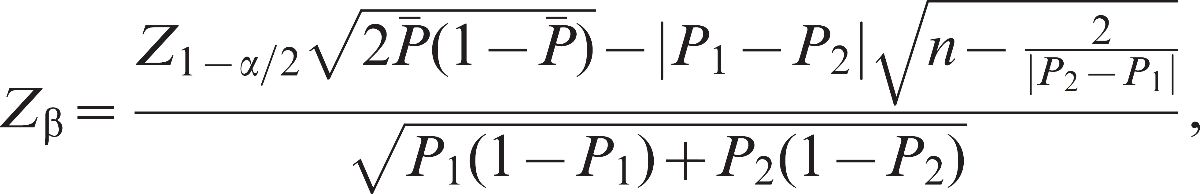
where n is the sample size, P1 and
P2 are the expected proportions in each group, and
is
the simple average of the expected proportions. Variables Z1–α/2
and Zβ are standard normal Z values. Power is
determined as 1 – cumulative probability associated with Zβ as
calculated from the formula (Table
7). Typical presentations of these formulas
24
incorporate
Zα/2 and addition of the numerator components.
An example would be to compare diagnostic sensitivity between 2 tests when both tests were
independently performed on 100 infected animals. Assume that the tests are believed to have
sensitivities of 85% and 90%, and a test with an alpha of 5% is desired. Epi Info 6 can be
used to calculate the power of the test to compare these 2 proportions. From the menu,
choose
Common standard normal Z scores for use in sample size formulas and power estimation.*
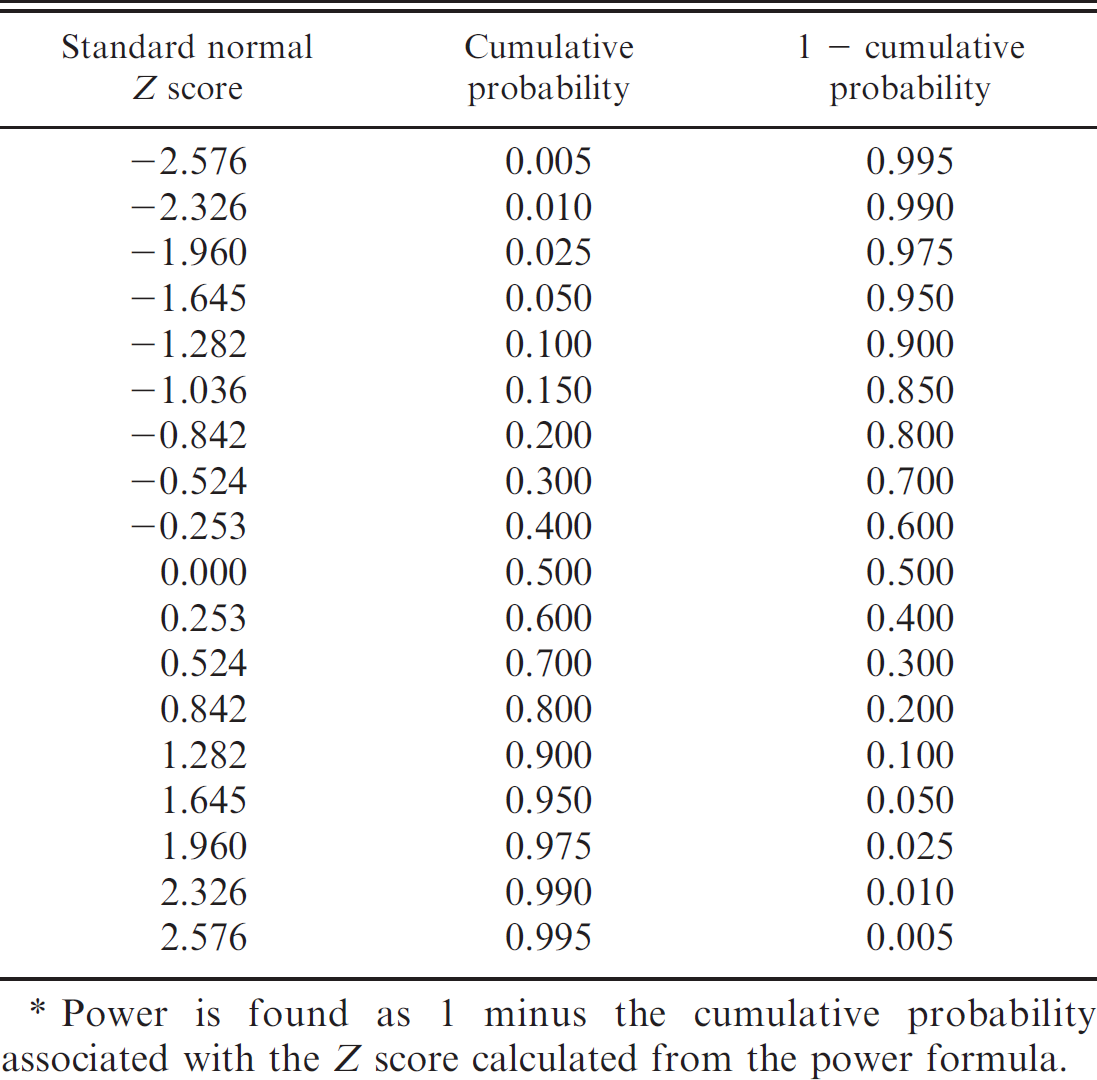
Power is found as 1 minus the cumulative probability associated with the Z score calculated from the power formula.
The calculation of power is dependent on the specification of an alternative hypothesis. The sampling distribution of the proportion under the null hypothesis is determined, and the critical value (Pr Z ≤ z = 1 – α/2) is located on this distribution. The alternative hypothesis is set as the expected difference in the 2 population proportions, and the sampling distribution of this difference is plotted with the critical value under the null hypothesis. The area under the sampling distribution of the alternative hypothesis to the right of the critical value is the power of the statistical test (Fig. 5). The shapes of these curves depend on the hypothesized proportions and the sample size. There is only a single power value related to each possible alpha and alternative hypothesis (expected difference in proportions).
Conclusions
The calculation of the sample size is very important during the design stage of all epidemiologic studies and should match the proposed statistical analysis to the extent possible. It is important to recognize that there is no single correct sample size, and all calculations are only as good as the employed assumptions. The sample size ensures statistical significance if the subsequent data collection is perfectly consistent with the assumptions made for the sample size calculation (assuming power was set as 50% or greater). If the null hypothesis is false and the assumed alternate hypothesis is true, then the probability of observing statistical significance will be equal to the assumed power of the test. The choice of assumptions for calculations is very important because their validity determines the likelihood of observing statistical significance. The traditional choices of 5% alpha and 20% beta can simply be used unless the investigator has specific reasons for other values. The choices of the best guesses or hypothesized values for the proportions that will be estimated by the study are more difficult. Values for these assumptions should be based on available literature or expert opinion. When there is doubt concerning their value, then proportions could be assumed to be close to 0.5. A proportion of 0.5 has the maximum variance, and therefore would result in the largest sample size.
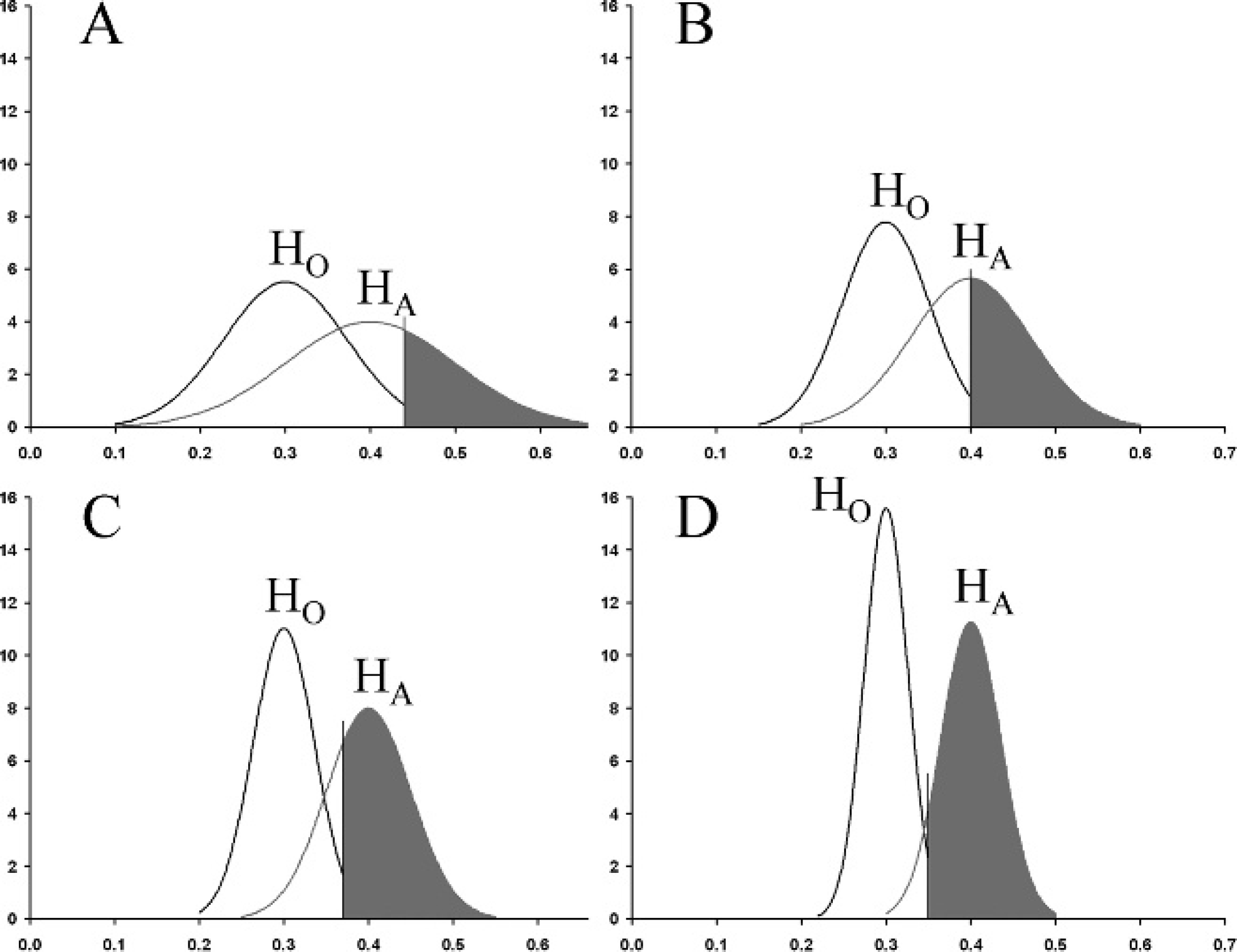
The sampling distribution under the null (black line) and alternative (gray line)
hypotheses for the situation when P1 = 0.2 and
P2 = 0.4 with equal group sizes. HO is the null
hypothesis that the true proportion is 0.3 (simple average of
P1 and P2), and HA
is the alternative hypothesis that P1 = 0.2 and
P2 = 0.4 and is centered at
P2. Alternatively, HA could have been centered at
P1. The gray shaded area corresponds to the power for the
statistical test with alpha of 5% when the sample size per group is 20 (
Sample size calculations correspond to the number of animals that are required to complete the study and be available for statistical analysis. They are the minimum sample sizes required to achieve the desired statistical properties. Sample size calculations should be increased by the number of animals that are anticipated to be lost during the study. The study design influences the number of animals expected to be lost during implementation. Cross-sectional studies should have minimal losses, but there is always the possibility of mislabeled samples, lost records, and laboratory errors. Sample sizes for cross-sectional studies should be increased 1–5% to account for these potential losses. Prospective studies that cover long time periods could have substantial losses, but these types of study designs are unusual for diagnostic investigations.
Some published recommendations include the post-hoc calculation of power when study results fail to achieve statistical significance. 34 However, there is no statistical basis for this calculation. 31 The power of a 2-sided test with an alpha set to be equal to the observed P value is typically 50%, 34 as presented in Figure 5. Therefore, post-hoc power calculations will typically be less than 50% for observed nonsignificant results. This fact, in conjunction with the one-to-one relationship between P value and power, suggests that little information can be garnered from their calculation. Post-hoc calculations of power could be useful if performed for magnitudes of differences other than what was observed by the study. In general, however, the post-hoc calculation of power is akin to determining the probability that an event will be observed after the event has already occurred (or not).
A primary purpose of sample size calculations is to ensure that the proposed study will be of an appropriate size to find an important difference statistically significant. Therefore, calculations should be performed prior to the determination of the study size. In practice, however, sample sizes are sometimes performed after the number of animals for study has been set, for reasons that might include cost or availability. Often, the assumptions are simply modified based on trial and error until calculations lead to the predetermined sample size, and these calculations are presented in grant applications or other proposed research plans. Also, studies are sometimes performed without performing any sample size calculations. Many journals require discussion of sample size calculations, and therefore such calculations are sometimes performed after the fact, with assumptions modified until the appropriate size is found. These are obviously not appropriate uses of sample size calculations. A better approach often would be the calculation of power based on the sample size expected to be used for the study. Though such post-hoc determinations are inappropriate or misleading, many epidemiologists and statisticians likely have been asked to perform these calculations. Unfortunately, the realities of research do not always coexist peacefully within the service of science itself. It is hoped that the material presented in the present article will demystify sample size calculations and encourage their use during the initial design phase of surveillance and diagnostic evaluations.
Acknowledgements
This manuscript was prepared in part through financial support by the U.S. Department of Agriculture, Cooperative State Research, Education, and Extension Service, National Research Initiative Award 2005–35204–16087. The author would like to thank the anonymous reviewers for helpful suggestions, which resulted in a better overall paper.