Sage Journals: Discover world-class research

Abstract

Geometric deviation, defined as the distance between the designed surface and the machined surface, is an important component of machining errors in five-axis flank milling of the S-shaped test piece. Since the interpolated toolpath in practical machining process is the approximation of the theoretical toolpath, the geometric deviation caused by the interpolated toolpath appears. To overcome this problem, a novel geometric deviation reduction method is suggested in this study. First, the features of the S-shaped test piece are analyzed. Second, the theoretical toolpath is generated according to the designed surface and the cutter location data is obtained by discretizing the theoretical toolpath. The linear interpolation of the cutter location data is carried out to obtain the interpolated toolpath. Then, the geometric deviation is modeled by calculating the Hausdorff distance between the tool axis trajectory surface based on the interpolated toolpath and the offset surface of the designed surface. Finally, the geometric deviation is reduced by optimizing the cutter location data without inserting more cutter location points. The machining experiment is conducted to verify the effectiveness of the proposed method. The experimental results agree with the simulation results, and both of them indicate the geometric deviation on the machined surface reduces after optimization.

Keywords

Five-axis flank milling geometric deviation interpolated toolpath cutter location data optimization S-shaped test piece

Introduction

The S-shaped test piece is a standard test piece for accuracy detection of five-axis machine tools. The toolpath of cutter motion has an important effect on the machining error in five-axis flank milling of theS-shaped test piece.^1,2 The theoretical toolpath (TTP) is a continuous curve offsetting a distance of cutter radius from the designed surface.³ However, since current machine tools cannot follow the TTP continuously, the TTP is discretized as cutter location (CL) data. The practical interpolated toolpath (PITP) is the result of linear interpolation of the CL data.⁴ The approximation of TTP by the CL data causes the misalignment between the TTP and PITP, which can be called as geometric deviation.^5,6

Many works have been done to reduce the machining error between the TTP and PITP. In these works, different interpolation algorithms for interpolated toolpath were proposed.⁷ Zhang et al.⁸ presented a parametrical cubic spline curve transitional approach for the interpolation of continuous short line segments. The trajectory error of the transitional curve is deduced according to the constraints of control points. Li et al.⁹ proposed a real-time and look-ahead interpolation algorithm for machining of micro-line segments under the chord error and drive axes constraints. Tajima and Sencer¹⁰ controlled the contouring errors at sharp corner of the linear segmented toolpath by interpolating axis velocity and accelerations accurately from the start to the end of the corner. However, their works focus on the toolpath in two-dimensional space. For the complex toolpath in three-dimensional space, the interpolation algorithms are more complex. Shi et al.¹¹ proposed a pair of quantic Pythagorean-hodograph (PH) curves to round the corners of five-axis toolpath, and those two rounded curves are synchronized linearly in interpolation according to the accuracy requirements of the tool tip and tool orientation tolerances. Bi et al.¹² used one cubic Bezier curve to interpolate the segments junction of the line toolpath for the tool tip points and the other one cubic Bezier curve to interpolate the segments junction of the rotational toolpath for the tool orientations. However, the aforementioned interpolation algorithms are for the micro-line segments at the corners of the toolpath. The derivatives of the toolpath at these junctions are discontinuous. On the contrary, the S-shaped test piece is constructed by the spline curves that have continuous derivative. Therefore, the interpolation algorithms for fitting the toolpath whose derivatives are discontinuous are not suitable for the toolpath of the S-shaped test piece.

The machining error induced by misalignment between the differentiable spatial curve and the PITP is investigated in recent works.¹³ Tajima and Sencer¹⁴ proposed a novel real-time trajectory generation technique for accurate tool tip interpolation of discrete five-axis machining toolpath with the control of tool tip and tool orientation errors. Wang et al.¹⁵ converted B-spline to piecewise power basis functions to establish formulas for computing interpolation points explicitly without calculating the chord error. To reduce the chord error, CL data densification is an effective method. Msaddek et al.¹⁶ suggested a simulation methodology for chord error caused by the B-spline interpolation and C-spline interpolation. Then, they compensated the machining errors between the spline trajectories and the theoretical trajectory by using insertion of the control nodes.¹⁷ Zhu et al.¹⁸ developed a method for correcting the numerical control codes to compensate for the geometric deviation of the toolpath. Li et al.¹⁹ densified the CL data to reduce the non-linear error at the connection points of line segments. The tool tip center (TTC) points are computed by the cubic spine interpolation, and the tool posture vectors are obtained via linear interpolation. However, the aforementioned works are concerned with the toolpath of the end milling freeform surface, and the machining error caused by the flank side of the tool is not considered. Besides, the data densification makes the toolpath planning complicated. To deal with these problems, the geometric deviation distributed in the three-dimensional space in five-axis flank milling of the S-shaped test piece is studied in this article.

In this study, the geometric deviation caused by the PITP in five-axis flank milling of the S-shaped test piece is considered directly when the tool feeds from one CL to the next consecutive CL. A new geometric deviation estimation model is proposed; subsequently, the geometric deviation is reduced directly by optimizing the CL data without inserting more CL points. The CL data are optimized by modifying the TTC point and the tool end center (TEC) point of intermediate tool axis of three consecutive tool axes. The remaining of this study is organized as follows: the features of the S-shaped test piece are analyzed in section “Features of the S-shaped test piece.” The geometric deviation estimation model is proposed in section “Geometric deviation estimation model.” Section “Geometric deviation reduction method” shows the geometric deviation reduction method. Simulation and experimental validations are provided in section “Simulation and experiment,” with the conclusions presented in section “Conclusion.”

Features of the S-shaped test piece

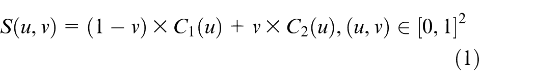
The side surfaces of the S-shaped test piece are two undevelopable ruled surfaces. They are named surface S₁ and surface S₂ in this study, respectively, as shown in Figure 1. Two regions with the maximum curvature on each ruled surface are termed region R₁ and region R₂. The equation of undevelopable ruled surface is defined as

S (u, v) = (1 - v) \times C_{1} (u) + v \times C_{2} (u), (u, v) \in {[0, 1]}^{2}

(1)

Figure 1.

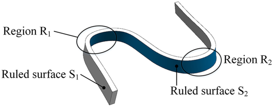
The S-shaped test piece and regions R₁ and R₂.

where S(u, v) represents any point on the ruled surface and it is decided by parameters u and v; C₁(u) and C₂(u) are two quasi-uniform cubic rational B-splines of each ruled surface, that is, two boundary curves of the ruled surface.

The equation of the B-spline is defined as

C (u) = \sum_{i = 0}^{k} P_{i} N_{i, n} (u)

(2)

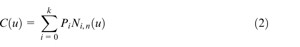
where P_i (i = 0, 1,…, k) denotes the control points of the B-spline;¹N_i,n(u) represent the basis functions referring to the De Boor–Cox method, and n is the order of the B-spline.

The ruled surface can be seen as a straight line moves along the boundary curves. The straight line is called the ruled line, and the boundary curves are called the guiding curves, corresponding to parameters u and v, respectively. Therefore, the parameter equations of the ruled surface can be expressed as

u = u (t), v = v (t)

(3)

where u(t) and v(t) are continuously differentiable functions.

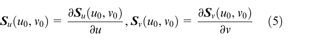
For any point Q(u₀, v₀) on the ruled surface S(u, v), the unit normal vector is expressed as

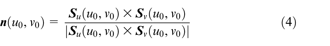
n (u_{0}, v_{0}) = \frac{S_{u} (u_{0}, v_{0}) \times S_{v} (u_{0}, v_{0})}{| S_{u} (u_{0}, v_{0}) \times S_{v} (u_{0}, v_{0}) |}

(4)

where S _u(u₀, v₀) and S _v(u₀, v₀) are the tangent vectors of the ruled surface. They are defined as

S_{u} (u_{0}, v_{0}) = \frac{\partial S_{u} (u_{0}, v_{0})}{\partial u}, S_{v} (u_{0}, v_{0}) = \frac{\partial S_{v} (u_{0}, v_{0})}{\partial v}

(5)

The parameter equation of the normal line passing through point Q(u₀, v₀) is expressed as

P (t) = Q (u_{0}, v_{0}) + t n (u_{0}, v_{0})

(6)

where t is the parameter of any point on the normal line.

Geometric deviation estimation model

Toolpath generation

The double points offset (DPO) method is adopted in this study to obtain the TTP, as illustrated in Figure 2. The basic idea is offsetting a distance of cutter radius r from two cutter contract (CC) points Q₁ and Q₂ on the guiding curves C₁(u) and C₂(u) in the direction of the unit normal vectors passing through the CC points. Supposing the TTC point corresponds to the guiding curve C₂(u), the tool axis unit vector v _t is expressed as

v_{t} = \frac{r n_{e} (u_{0}) - r n_{t} (u_{0})}{‖ r n_{e} (u_{0}) - r n_{t} (u_{0}) ‖}

(7)

Figure 2.

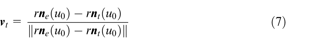
Toolpath generation using the DPO method.

where r n _t(u₀) is the TTC point radius vector and r n _e(u₀) is the TEC point radius vector.

The CL data are obtained by discretizing the TTP. The TTC points and the TEC points can be transformed into the TTC points and the corresponding tool axis vectors.

Estimation of the geometric deviation

When the CL data are obtained from the TTP, the computer numerical control (CNC) system drives the machine by reading the CL data. If the cutter moves in the two-dimensional plane, the TTP T_o(u) is the offset curve $T_{1} T_{3}$ of the curve C(u), as shown in Figure 3. The PITP T(u) includes the line segments $\bar{T_{1} T_{2}}$ and $\bar{T_{2} T_{3}}$ . For any TTC point T_i on the TTP T_o(u), the geometric deviation e, that is, the chord error is the perpendicular distance between point T_i and line segment $\bar{T_{1} T_{2}}$ . The two-dimensional geometric deviation is expressed as

e = \frac{T_{1} T_{i} \times T_{1} T_{2}}{| T_{1} T_{2} |}

(8)

Figure 3.

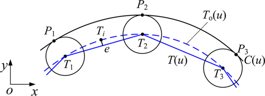
Two-dimensional geometric deviation on the projection of the cutter cross section.

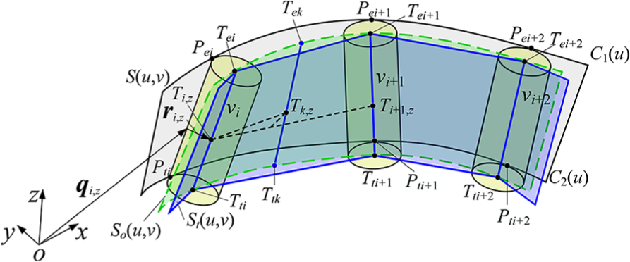
The chord error is expanded to the three-dimensional space to estimate the geometric deviation in the flank milling. Any three consecutive CLs are taken to derive the three-dimensional geometric deviation, as shown in Figure 4. P_ti, P_ti₊₁ and P_ti₊₂ are three consecutive CC points on curve C₂(u), and P_ei, P_ei₊₁ and P_ei₊₂ the CC points on curve C₁(u). T_ti, T_ti₊₁ and T_ti₊₂ are three consecutive TTC points on the tool axis trajectory surface S_t(u, v), and T_ei, T_ei₊₁ and T_ei₊₂ are TEC points. The equation of the offset surface S_o(u, v) of the designed surface is expressed as

S_{o} (u, v) = S (u, v) + r n (u, v)

(9)

The tool axis trajectory surface S_t(u, v) is the shape when the cutter moves along the PITP. When the CNC system reads the CL data, regardless of which interpolation method the CNC system adopts, the tool feeds along the micro-lines after interpolation. Because the interpolation process employs tiny straight segments to approximate the curve. The tool axis trajectory surface S_t(u, v) involves line segments $\bar{T_{ti} T_{ti + 1}}$ and $\bar{T_{ei} T_{ei + 1}}$ . The line segments have a deviation with the offset surface S_o(u, v) involving curves $T_{ti} T_{ti + 1}$ and $T_{ei} T_{ei + 1}$ . The distance between the tool axis trajectory surface and the offset surface is defined as the geometric deviation in flank milling between two consecutive CLs.

Figure 4.

The geometric deviation in flank milling between two consecutive tool axes v _i and v _i+1.

The geometric deviation between two consecutive CLs influences the machining accuracy directly. The maximum geometric deviation is calculated using the Hansdorff distance. The Hausdorff distance from point set M to point set N is defined as

h (M, N) = \max_{m \in M} \min_{n \in N} {d (m, n)}

(10)

where m and n are points in sets M and N, M = {m₁, m₂,…, m_m} and N = {n₁, n₂,…, n_n}, respectively; d(m, n) represents the Euclidean distance between sets M and N.

The calculation of the geometric deviation includes three steps as follows. The first step is to define the sets M and N. For any parameter $v_{i} \in [0, 1]$ , the normal surface S_n(u, v_i) is composed of the normal vectors n (u, v_i). The intersection points of normal surface S_n(u, v_i) and the offset surface S_o(u, v) are set M. The intersection points of normal surface S_n(u, v_i) and the practical tool axis trajectory surface S_t(u, v) are set N. They are described as

M = S_{n} (u, v_{i})) \cap S_{o} (u, v), N = S_{n} (u, v_{i}) \cap S_{t} (u, v)

(11)

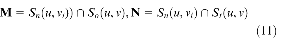
The second step is calculating the Euclidean distance between sets M and N. For any two consecutive tool axes v _i and v _i+1, as shown in Figure 4, the theoretical tool axis v _k on the TTP is taken to calculate the geometric deviation. Supposing parameter v_i equals v_z, points T_i,z, T_i+_1,z and T_k,z are the corresponding points on the tool axes. The distance between sets M and N is expressed as

\begin{matrix} e_{p} = \frac{T_{i, z} T_{k, z} \times T_{i, z} T_{i + 1, z}}{| T_{i, z} T_{i + 1, z} |} = \frac{[(q_{i, z} + r_{i, z}) - (q_{k, z} + r_{k, z})] \times [(q_{i, z} + r_{i, z}) - (q_{i + 1, z} + r_{i + 1, z})]}{| (q_{i, z} + r_{i, z}) - (q_{i + 1, z} + r_{i + 1, z}) |}, k \in [i, i + 1] \end{matrix}

(12)

where q _i,z and q _i+1,z are the vectors pointing from origin o to the CC points corresponding to tool axes v _i and v _i+1 at a height of z; q _k,z is the vector pointing from origin o to the CC point corresponding to the theoretical tool axis v _k at a height of z; r _i,z and r _i+1,z denote the cutter radius vectors of tool axes v _i and v _i+1 at a height of z; r _k,z is the cutter radius vector of theoretical tool axis v _k at a height of z (for convenience, only vectors q _{i, z} and r _{k, z} are shown in Figure 4, the others are similar).

Substituting equation (12) into equation. (10), the Hausdorff distance between two consecutive CLs with a specific parameter v_z is obtained. If the tool axis trajectory surface locates between the offset surface and the designed surface, the workpiece is overcut by the cutter; otherwise, the workpiece is undercut.

The third step is repeating the aforementioned steps for parameter $v_{i} \in [0, 1]$ to obtain the geometric deviation between two consecutive CLs. Repeating all the CLs, the geometric deviation distribution on the ruled surface is obtained.

Geometric deviation reduction method

This section proposes a CL data optimization method to reduce the three-dimensional geometric deviation in flank milling.

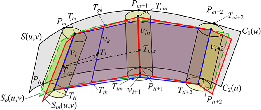
For any three consecutive CLs shown in Figure 5, the original TTC points and the tool axis vectors before optimization are described in section “Geometric deviation estimation model.” Since tool axis vectors v _i and v _i+1 are offset from the designed surface, the geometric deviation in these two CLs is zero. Therefore, the geometric deviation changes from the minimum to the maximum and reduces to the minimum again when the tool feeds from one CL to the next consecutive CL, and the same trend occurs between any two consecutive CLs. To reduce the maximum geometric deviation between two consecutive CLs, the intermediate tool axis vector v _i+1 of three consecutive tool axis vectors v _i, v _i+1 and v _i+2 is modified by changing the TTC point and TEC point of vector v _i+1 simultaneously.

Figure 5.

Optimization of the CL data by modifying the intermediate tool axis vector v _i+1 of three consecutive tool axis vectors v _i, v _i+1 and v _i+2.

The tool axis vector v _i+1 locates in the theoretical position before optimization. This indicates that if its position or orientation changes, geometric deviation will occur in the location of tool axis vector v _i+1. However, two consecutive path segments in both sides of tool axis vector v _i+1 will change simultaneously. Therefore, the geometric deviation on the two consecutive path segments will change simultaneously. The geometric deviation on the path segment from the tool axis vectors v _i to v _i+1 is described in detail herein.

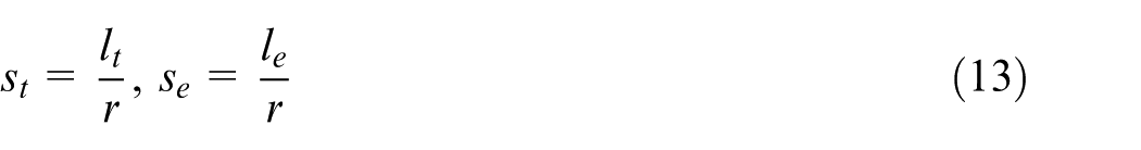
Supposing that the TTC point and TEC point changes in the direction or the inverse direction of the unit normal vector of the CC points P_ti₊₁ and P_ei₊₁. The ratios of the movement length l_t and l_d to the cutter radius r are defined as s_t and s_e pertaining to the TTC point and TEC point, respectively

s_{t} = \frac{l_{t}}{r}, s_{e} = \frac{l_{e}}{r}

(13)

When the TTC point and the TEC point change, the new tool axis becomes vector v _in and the new tool axis trajectory surface is adjusted to surface S_tn(u, v). The new tool axis trajectory surface S_tn(u, v) involves line segments $\bar{T_{ei} T_{ein}}$ and $\bar{T_{ti} T_{tin}}$ . Then, the geometric deviation after optimization is calculated using Hausdorff distance between the offset surface S_o(u, v) and the new tool axis trajectory surface S_tn(u, v). The new distance is expressed as

e_{pn} = \frac{T_{i, z} T_{k, z} \times T_{i, z} T_{in, z}}{| T_{i, z} T_{in, z} |} = \frac{((q_{i, z} + r_{i, z}) - (q_{k, z} + r_{k, z})) \times ((q_{i, z} + r_{i, z}) - (q_{i + 1, z} + r_{in, z}))}{| (q_{i, z} + r_{i, z}) - (q_{i + 1, z} + r_{in, z}) |}, k \in [i, i + 1]

(14)

where r _in,z is the new tool radius vector of tool axis v _in at a height of z. It is similar to vector r _i,z.

Substituting equation (14) into equation (10) and repeating three steps described in section “Estimation of the geometric deviation,” the new geometric deviation on the machined surface between two consecutive CLs is obtained.

The basic idea of reducing the geometric deviation is to find the minimum of e_pn by modifying the TTC point and the TEC point. The relationship between the maximum geometric deviation and parameters s_t and s_e is analyzed here. If the absolute values of parameters s_t and s_e are zero, the tool axis has no changes, and the tool axis is still the original tool axis. If the absolute values of s_t and s_e are very large, the tool axis changes a lot, which means the new PITP will deviate from the TTP obviously, causing the geometric deviation very large simultaneously. Therefore, the solutions of parameters s_t and s_e to make geometric deviation minimum exist. The bisection method is adopted to search the solution of parameters s_t and s_e. The solution of parameter s_t is searched first. Specifically, set parameter s_e and adjust parameter s_t. When the maximum geometric deviation is minimum, the solution of parameter s_t is obtained. The solution of parameter s_e is found in the same way. Thus, a solution of parameters s_t and s_e is obtained.

Simulation and experiment

Numerical simulation

The simulation parameters are the same as those in experiment. The height of the S-shaped test piece is 30 mm. The milling width a_e is 10 mm in the practical flank milling process. So, it is divided into three cutting layers. The radius r of the cylindrical cutter is 10 mm. The simulation results of the geometric deviation are described subsequently.

The three-dimensional geometric deviation between the offset surface and the tool axis trajectory surface on ruled surfaces S₁ and S₂ is simulated in MATLAB. The distributions of the geometric deviation before optimization on ruled surfaces S₁ and S₂ are shown in Figure 6. Figure 6(a) shows that the maximum overcut in region R₁ is 0.0313 mm, and the maximum undercut in region R₂ is −0.0230 mm on the ruled surface S₁. Figure 6(b) shows that the maximum overcut in region R₂ is 0.0239 mm, and the maximum undercut in region R₁ is −0.0123 mm on the ruled surface S₂.

Figure 6.

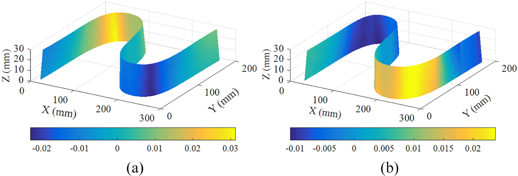
Distributions of three-dimensional geometric deviation in simulation on: (a) ruled surface S₁ and (b) ruled surface S₂ before optimization.

The CL data are optimized using the proposed TTC points and TEC points modification method. For the flank milling of ruled surface S₁, parameters s_t and s_e are 0.070 and 0.072 that can make geometric deviation minimum. For the flank milling of ruled surface S₂, they are 0.075 and 0.070. The distributions of the geometric deviation on ruled surfaces S₁ and S₂ are shown in Figure 7.

Figure 7.

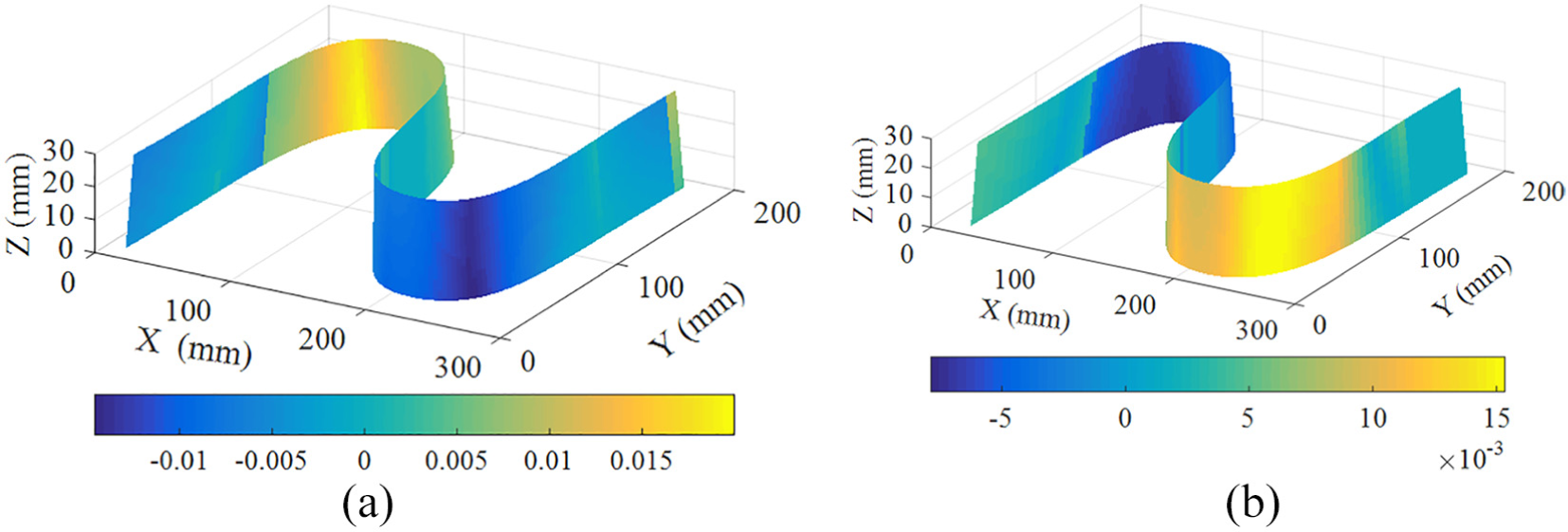
Distributions of three-dimensional geometric deviation in simulation on: (a) ruled surfaces S₁ and (b) ruled surface S₂ after optimization.

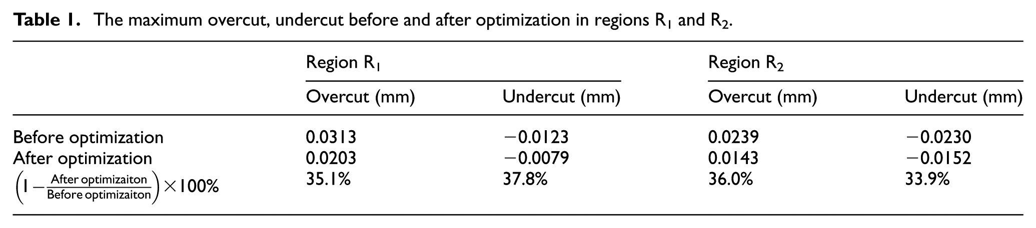
Figure 7(a) shows that the maximum overcut in region R₁ is 0.0203 mm, and the maximum undercut in region R₂ is −0.0153 mm on ruled surface S₁ after optimization. The maximum overcut and undercut on ruled surface S₁ reduce 35.1% and 37.8%, respectively. Figure 7(b) shows that the maximum undercut in region R₁ is −0.0079 mm, and the maximum overcut in region R₂ is 0.0152 mm on ruled surface S₂ after optimization. The maximum overcut and undercut on ruled surface S₂ reduce 36.0% and 33.9%, respectively. The simulation results are summarized in Table 1.

Table 1.

The maximum overcut, undercut before and after optimization in regions R₁ and R₂.

	Region R₁		Region R₂
	Overcut (mm)	Undercut (mm)	Overcut (mm)	Undercut (mm)
Before optimization	0.0313	−0.0123	0.0239	−0.0230
After optimization	0.0203	−0.0079	0.0143	−0.0152
$(1 - \frac{After optimizaiton}{Before optimizaiton}) \times 100 %$	35.1%	37.8%	36.0%	33.9%

To compare the geometric deviation before and after optimization more clearly, the geometric deviation in regions R₁ and R₂ is discussed in detail. The parameter v equals to 0.8333 of the ruled line is selected to analyze the geometric deviation. It corresponds to the height z = 25 mm of the ruled surface in the workpiece coordinate frame. The distributions of the geometric deviation along the guiding line in regions R₁ and R₂ are shown in Figure 8.

Figure 8.

Distributions of geometric deviation with z = 25 mm in regions: (a) R₁ and (b) R₂.

The geometric deviation on ruled surfaces S₁ and S₂ reaches maximum in regions R₁ and R₂, respectively. The peak geometric deviation is about 0.03 mm. It is so large for two reasons. One is that the curvature in these regions is the largest. The other reason is that the practical tool motion is along the micro-line. The bigger the curvature is, the bigger the geometric deviation is. They are the main sources of the peak geometric deviation. Figure 7 shows that the geometric deviation is smaller than 0.01 mm on most regions of the ruled surface. Next, the geometric deviation in regions R₁ and R₂ is verified in the cutting experiment.

Experiment

Experimental conditions

The proposed CL data optimization method is experimentally verified on an A/C table-tilting five-axis CNC machining tool VMC 0656, as shown in Figure 9(a). The machined surfaces are measured on the coordinate measurement machine (CMM) ZEISS CONGURA G2, as shown in Figure 9(b). The material of the S-shaped test piece is Al-7075-T7451 aluminum alloy. The machining deformation in the machining process is excluded here. The machining deformation error is about 0.008 mm in regions R₁ and R₂ when the thickness of the S-shaped test piece is 4 mm.²⁰ To eliminate the effect of workpiece deformation, the thickness of the S-shaped test piece is designed as 10 mm in this study. The cylindrical cutter with two teeth is a straight-end high speed steel milling cutter. The tool cutting edge length is 75 mm. The cutting parameters include a feed rate of 300 mm/min and a spindle speed of 6000 r/min. The heights of three machining layers are 20, 10 and 0 mm in the workpiece coordinate frame.

Figure 9.

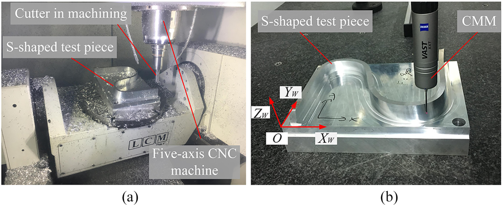
(a) Machining process on the five-axis CNC machine tool and (b) measurement on the CMM.

The geometric deviation in this study is described and measured in the workpiece coordinate frame. The CL data include the TTC points P = [P_x P_y P_z]^T and the tool axis vectors O = [O_i O_j O_k]^T in the workpiece coordinate frame. However, the five-axis machine tool motion commands q = [x, y, z, θ_a, θ_c]^T, including three translational axes and two rotary axes, are described in the machine coordinate system. Therefore, the CL data need to be transformed into the motion commands. Three translational motion commands are transformed using TTC points directly. Considering forward kinematics, two rotary motion commands corresponding to the tool axis vectors are obtained using the following transformation formula

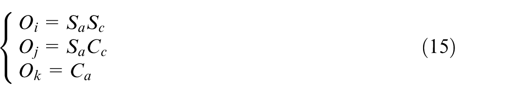
{\begin{matrix} O_{i} = S_{a} S_{c} \\ O_{j} = S_{a} C_{c} \\ O_{k} = C_{a} \end{matrix}

(15)

where S_a = sin(θ_a), C_a = cos(θ_a), S_c = sin(θ_c) and C_c = cos(θ_c).

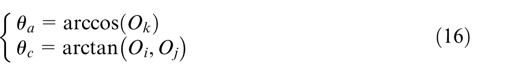
The displacements of rotary axes A and C are obtained from the inverse kinematics solved from equation (15) and are expressed as

{\begin{matrix} θ_{a} = \arccos (O_{k}) \\ θ_{c} = \arctan (O_{i}, O_{j}) \end{matrix}

(16)

Two rotary motion commands of the table-tilting table when machining first layer of ruled surface S₂ are shown in Figure 10, which are similar to that of the other layers.

Figure 10.

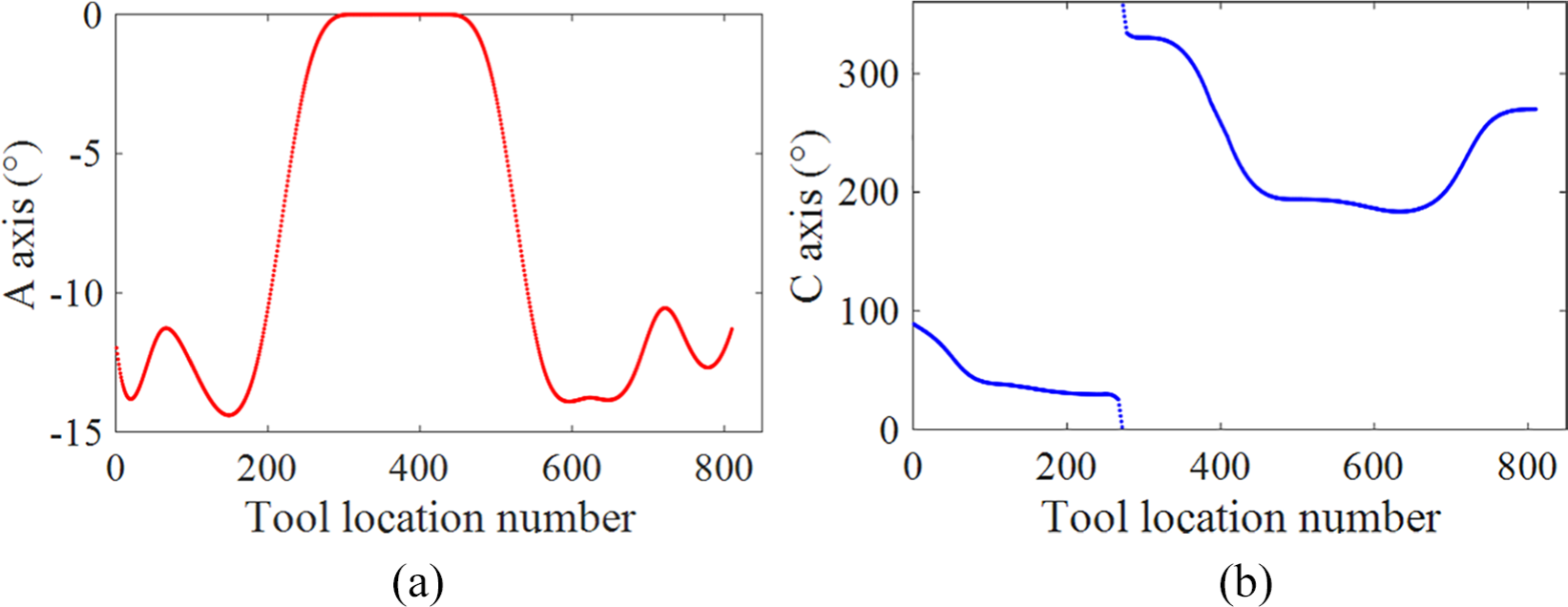
Motion commands for (a) A axis and (b) C axis when machining first layer of ruled surface S₂.

Experiment results and discussions

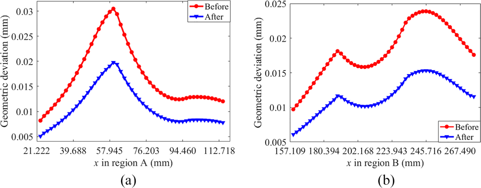
Two S-shaped test pieces before and after the CL data optimization are cut. The geometric deviation of the machined surface with z = 25 mm is measured, as shown in Figure 11. The measurement results of geometric deviation in regions R₁ and R₂ before and after optimization are shown in Figure 12.

Figure 11.

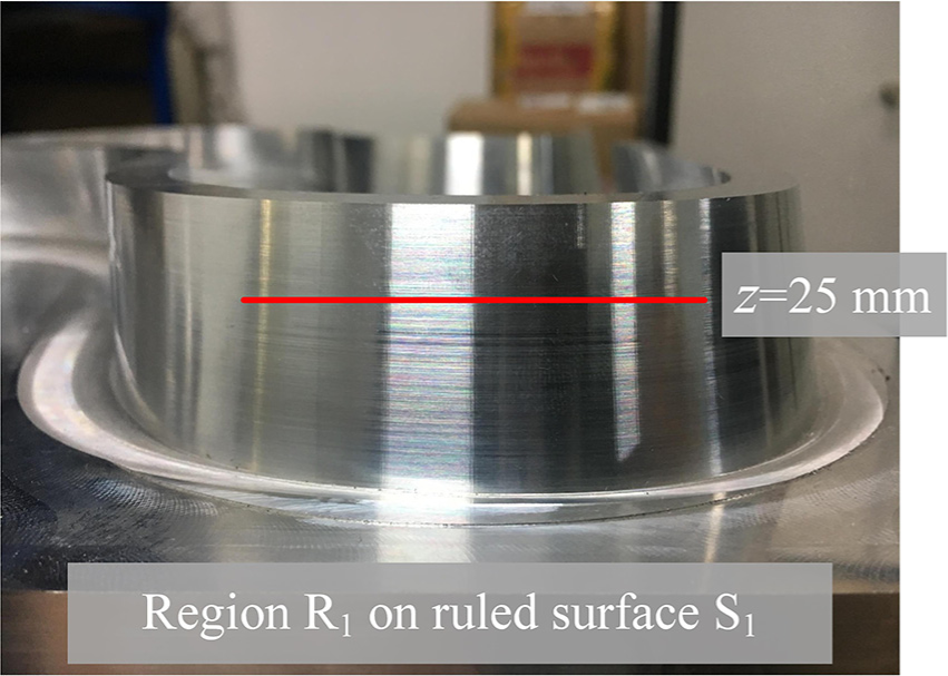
The measurement height z = 25 mm in region R₁ on the machined surface S₁.

Figure 12.

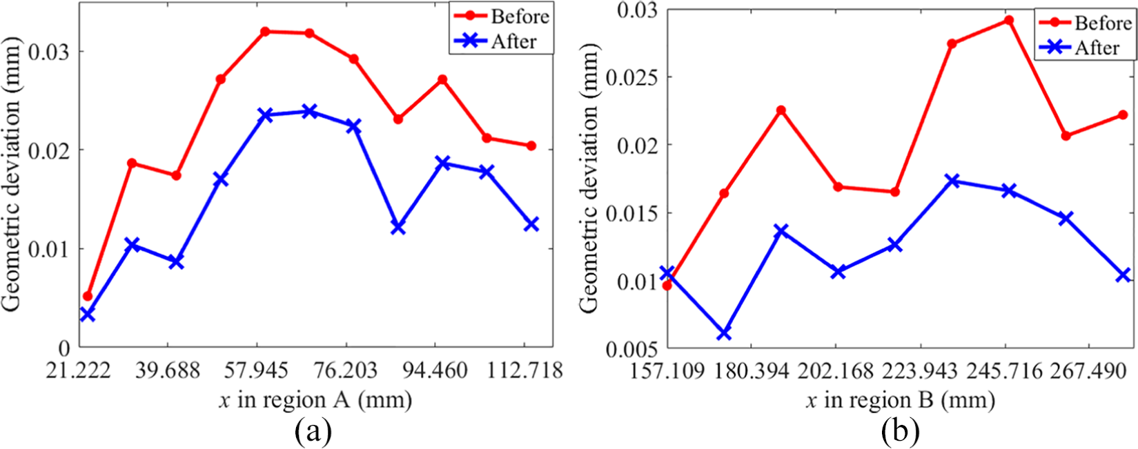
Geometric deviation on the machined surface: (a) in region R₁ and (b) in region R₂.

The measurement results of the machining experiment show that the practical geometric deviation on the machined ruled surfaces S₁ and S₂ have a trend similar to that of the simulated geometric deviation. Furthermore, the maximum geometric deviation on the machined surface in region R₁ before and after optimization is 0.0320 and 0.0239 mm, respectively, indicating a reduction of 25.3%. It is 0.0292 and 0.0173 mm in region R₂, respectively, indicating a reduction of 40.8%.

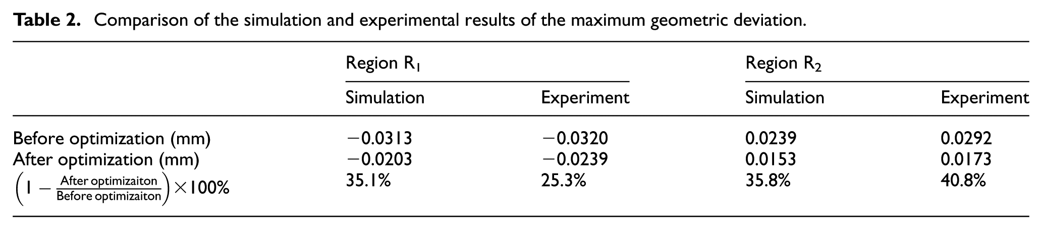
A comparison of the simulation results and the experimental results of the maximum geometric deviation in regions R₁ and R₂ is presented in Table 2. The effectiveness of the proposed geometric deviation reduction method by modifying the practical CL data is verified by both simulation results and the experimental results.

Table 2.

Comparison of the simulation and experimental results of the maximum geometric deviation.

	Region R₁		Region R₂
	Simulation	Experiment	Simulation	Experiment
Before optimization (mm)	−0.0313	−0.0320	0.0239	0.0292
After optimization (mm)	−0.0203	−0.0239	0.0153	0.0173
$(1 - \frac{After optimizaiton}{Before optimizaiton}) \times 100 %$	35.1%	25.3%	35.8%	40.8%

Conclusion

A new geometric deviation estimation model and reduction approach for five-axis flank milling of the S-shaped test piece is proposed in this article. The geometric deviation is caused by the fact that the machine tools cannot synchronize the practical cutter motion and the TTP. Actually, The CL data are used in the practical machining process. This study focuses on the geometric deviation based on the PITP to improve the motion accuracy when tool feeds from one CL to the next consecutive CL. The CL data are optimized to reduce the geometric deviation. Several distinct features of the proposed method are presented as follows.

The geometric deviation on the ruled surface between two consecutive CLs is studied directly. It is estimated by calculating the distance between the offset surface of the designed surface and the tool axis trajectory surface.

The geometric deviation is reduced by modifying the TTC point and TEC point to optimize the CL data. The proposed method is verified in simulation and machining experiment. The experimental results of geometric deviation meet that of the simulation results. Both results indicate that the geometric deviation reduces significantly by using the proposed method. Thus, the validity of the proposed method is verified.

This study provides an off-line CL data optimization method for improving the accuracy in five-axis flank milling of the S-shaped test piece. The proposed method is robust and effective. It leads to several potential topics in future work, such as feed rate control and the deformation of workpiece in the flank milling of the thin-walled parts.

Footnotes

Appendix 1 Declaration of conflicting interests

The author(s) declared no potential conflicts of interest with respect to the research, authorship, and/or publication of this article.

Funding

The author(s) disclosed receipt of the following financial support for the research, authorship, and/or publication of this article: This work was supported by the Major national science and technology projects of China under grant no. 2017ZX04002001 and the National Natural Science Foundation of China under grant no. 51975319.

ORCID iD

Hao Si

References

Guan

, et al. An improved positioning method for flank milling of S-shaped test piece. Int J Adv Manuf Technol 2017; 92(1–4): 1349–1364.

Chen

Sun

, et al. Measurement and analysis for frequency domain error of ultra-precision spindle in a flycutting machine tool. Proc IMechE, Part B: J Engineering Manufacture 2018; 232(9): 1501–1507.

Magalhaes

Ferreira

JCE

. Assessment of tool path strategies for milling complex surfaces in hardened H13 steel. Proc IMechE, Part B: J Engineering Manufacture 2019; 233(3): 834–849.

Tutunea-Fatan

Feng

HY.

Determination of geometry-based errors for interpolated tool paths in five-axis surface machining. J Manuf Sci Eng 2005; 127(1): 60–67.

Zhou

Chen

Yang

An accurate, efficient envelope approach to modeling the geometric deviation of the machined surface for a specific five-axis CNC machine tool. Int J Mach Tools Manuf 2015; 95: 67–77.

Zhu

LM.

Compensation of deformation errors in five-axis flank milling of thin-walled parts via tool path optimization. Precis Eng 2019; 55: 77–87.

Cai

Liu

Shi

, et al. Optimum end milling tool path and machining parameters for micro Laval nozzle manufacturing. Proc IMechE, Part B: J Engineering Manufacture 2017; 231(10): 1703–1712.

Zhang

You

, et al. The transition algorithm based on parametric spline curve for high-speed machining of continuous short line segments. Int J Adv Manuf Technol 2011; 52(1–4): 245–254.

Rastegar

, et al. A real-time and look-ahead interpolation algorithm with axial jerk-smooth transition scheme for computer numerical control machining of micro-line segments. Proc IMechE, Part B: J Engineering Manufacture 2019; 233(9): 2007–2019.

10.

Tajima

Sencer

Kinematic corner smoothing for high speed machine tools. Int J Mach Tools Manuf 2016; 108: 27–43.

11.

Shi

Zhu

, et al. Corner rounding of linear five-axis tool path by dual PH curves blending. Int J Mach Tools Manuf 2015; 88: 223–236.

12.

Shi

Wang

, et al. Analytical curvature-continuous dual-Bézier corner transition for five-axis linear tool path. Int J Mach Tools Manuf 2015; 91: 96–108.

13.

Huang

Zhu

, et al. Third-order chord error estimation for freeform contour in computer-aided manufacturing and computer numerical control systems. Proc IMechE, Part B: J Engineering Manufacture 2019; 233(3): 863–874.

14.

Tajima

Sencer

Accurate real-time interpolation of 5-axis tool-paths with local corner smoothing. Int J Mach Tools Manuf 2019; 142: 1–15.

15.

Wang

Liu

, et al. Research of the real-time interpolation based on piecewise power basis functions. Proc IMechE, Part B: J Engineering Manufacture 2019; 233(3): 889–899.

16.

Msaddek

Bouaziz

Baili

, et al. Simulation of machining errors of Bspline and Cspline. Int J Adv Manuf Technol 2017; 89(9–12): 3323–3330.

17.

Msaddek

Baili

Bouaziz

, et al. Compensation of machining errors of Bspline and Cspline. Int J Adv Manuf Technol 2018; 97(9–12): 4055–4064.

18.

Zhu

Ding

Qin

, et al. Integrated geometric error modeling, identification and compensation of CNC machine tools. Int J Mach Tools Manuf 2012; 52(1): 24–29.

19.

Zhouyang

Lou

Tool path optimization in postprocessor of five-axis machine tools. Int J Adv Manuf Technol 2013; 68(9–12): 2683–2691.

20.

Wang

Error compensation in the five-axis flank milling of thin-walled workpieces. Proc IMechE, Part B: J Engineering Manufacture 2019; 233(4): 1224–1234.

Geometric deviation reduction method for interpolated toolpath in five-axis flank milling of the S-shaped test piece

Abstract

Keywords

Introduction

Features of the S-shaped test piece

Geometric deviation estimation model

Toolpath generation

Estimation of the geometric deviation

Geometric deviation reduction method

Simulation and experiment

Numerical simulation

Experiment

Experimental conditions

Experiment results and discussions

Conclusion

Footnotes

Appendix 1

Declaration of conflicting interests

Funding

ORCID iD

References