
Abstract
Cutter displacements and deflections induce a significant amount of surface error in machined thin-walled parts and are a major obstacle to achieving higher productivity in a five-axis milling operation. In this study, a milling force model for the five-axis flank milling process was established and implemented by calculating and simulating the cutter dynamic displacement to investigate the dynamic response of ruled surface impeller blades in the milling process. A machining trajectory and related machining parameters were selected to calculate the dynamic milling forces in the X and Y directions for each analysis time using the calculation method. Using ANSYS software, the milling forces in three directions were input into the finite element model of the ball-end milling tool. The deformation was analyzed using post-processing for the ruled surface milling. Then, the milling parameters related to the dynamic displacement of the tool in the side milling blade were trained and optimized using a back-propagation neural network and particle swarm optimization algorithm during the side milling of the ruled surface. In addition, processing experiments were performed based on the optimized parameters. The blade roughness tests indicated that the surface quality was considerably improved after optimization, thus verifying the feasibility of the optimization method.
Keywords
Introduction
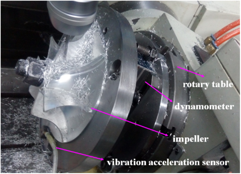
The required machining quality of integral impellers has significantly increased with the continuous development of aerospace technology. Among impeller parts, the ruled surface impeller is a particularly widely used form. Figure 1 shows the locations of the cutter and impeller blade during the milling process. However, the complex thin-walled curved surface of the blade makes it prone to deformation during processing, which affects the machining accuracy. Moreover, machining error is irreversible once it occurs. Many studies have been conducted to improve the machining quality of thin-walled parts, including studies on the dynamic milling force 1 and vibration 2 in the machining process of a thin-walled workpiece.
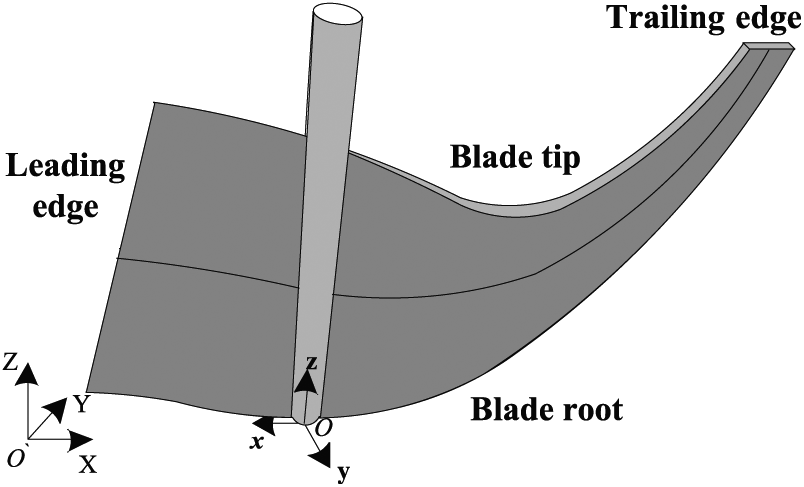
Locations of the cutter and blade during the milling process.
The dynamic characteristics of the spindle-tool system and the workpiece platform system significantly affect the machining process. The tool and workpiece system is a dynamic system in milling operations. Based on the stiffness characteristics, milling systems can be categorized as rigid workpiece–flexible cutter systems, rigid cutter–flexible workpiece systems or double flexible systems. Figure 2 shows a rigid workpiece–flexible cutter system, where the workpiece is considered rigid and the cutter is flexible.
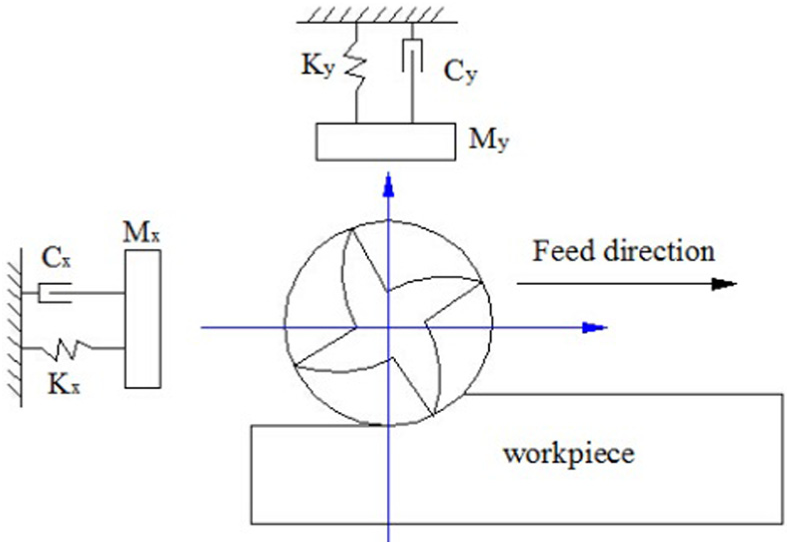
Rigid workpiece–flexible cutter system model.
Predicting the dynamic displacement in a flexible system is critical for achieving good machining quality and high productivity. Some studies have researched the flexible workpiece system. Using the one-degree-of-freedom model for a rigid cutter–flexible workpiece system, Peigne et al. 3 studied the dynamics of flank milling operations at low radial immersion milling rates. Izamshah et al. 4 developed a finite element analysis machining model to predict the distortion or deflection of thin-walled sections during the end milling process. Their model aimed to help with selecting the error compensation strategy when machining thin-walled metal structural components. In addition, the multiple regression analysis models for the deflection prediction were presented. 5
The dynamic displacement of a flexible tool is one of the main problems in the milling process. Many papers consider the displacement of the flexible cutter when studying the process stability of a milling system. Wojciechowski et al. 6 established a cutter displacement model with a variable inclined angle. In this model, the cutter displacement was separated into the displacement caused by the geometrical errors of the spindle-tool holder-milling tool system and the displacement caused by the cutting and centrifugal forces. Using the two-degree-of-freedom model for a flexible cutter system, Insperger et al. 7 obtained the cutter displacement in the milling process using the semi-discretization method to solve the differential equation. Seguy et al. 8 explored the relationship between chatter instability and surface roughness evolution for thin-wall milling. They obtained the cutter displacement by solving the nonlinear system of delay differential equations using the numerical integration method. In another study, the cutter displacement was calculated, and the dynamic characteristics of the cutter were investigated to estimate the cutting force. 9
Given the machining characteristics of the ruled surface in five-axis flank milling, this study considered the cutter and workpiece system to be a rigid workpiece–flexible cutter system. According to the characteristics of the cutter, the cutter was defined as a two-degree-of-freedom spring damping vibration system. The time-domain differential equations were solved using the fourth-order Runge–Kutta method after the second-order differential equation was transformed into a first-order equation.
In flank milling, the axial depth of a cut is typically quite large. Therefore, in this operation, the flexible cutter is highly prone to deformation, which could lead to unsatisfactory machining accuracy and surface quality. Research on predicting tool deformation could provide useful references and guidance for optimization techniques that can improve the surface quality of the workpieces. Sutherland and DeVor 10 proposed an iterative method for calculating the milling force and cutter deformation considering only the effect of tool deformation on instantaneous chip thickness. This method can be used to predict the milling force and surface error in milling processes with a flexible cutter. Dépincé and Hascoët 11 studied the influence of tool deformation on the workpiece in end milling. Tae-Jin et al. 12 used a finite element method (FEM) to analyze tool deformation. To model a discontinuous cutting force, Shi 13 modeled the concentrated shear stress using a discontinuous function for the cutting state and expressed the tool deformation and cutting force using a Fourier series. Kim et al. 14 presented a tool deflection model that considered the influence of surface inclination. Based on the dynamic milling force calculation of the processing time, this study simulated and analyzed the deformation and regularities of a cemented carbide ball-end milling cutter using the finite element software ANSYS 14.0 (ANSYS, Inc., USA).
The optimization of the computer numerical control (CNC) milling process includes optimizing both the machining path and machining parameters. Extensive research has been conducted on the generation and optimization of the machining path, leading to numerous achievements. However, few studies have focused on the optimization of the machining parameters. In certain previous studies, researchers optimized the machining parameters using the material removal rate to estimate the average milling force for the planning feed rate. Ferry and Altintas 15 presented an optimization process for the five-axis flank milling of jet engine impellers by automatically varying the feed rate as the tool–workpiece engagement. Budak and Altintas 16 established a method for identifying the optimal feed rate and cutting width by selecting appropriate cutting conditions to increase the material removal rate. Sungurtekin and Voelcker 17 highlighted the importance of the feed rate, which is determined by the milling force produced in the process. A similar conclusion was obtained by Vann and Cutkosky. 18 In terms of the modeling and simulation of the milling force, many parameter optimization studies used an instantaneous milling force model. Fussell et al., 19 Ko et al. 20 and Han and Cho 21 established an instantaneous milling force model by taking the milling force as a constraining condition and controlling the change in the instantaneous milling force in the milling process to optimize the feed rate. Establishing a stability-based selection method for the cutting parameters is important. Cao 22 proposed a method for selecting a reasonable spindle speed and cutting depth. In their method, the lower bound of the chatter stability lobe diagram and surface finish are taken as constraints, and the maximum material removal rate is set as the target.
This article proposes a new method for optimizing machining parameters. Orthogonal experiments were conducted to train the back-propagation (BP) neural network, and the machining parameters were optimized using a particle swarm optimization algorithm. The experimental machining results demonstrate that using optimized parameters can effectively improve the surface quality of the blade.
Simulation of the dynamic displacement response of a flexible tool system
In five-axis flank milling for a ruled surface blade, a cylindrical ball-end milling cutter with a lengthened shank is typically used to ensure that the fixture does not interfere with the edge of the blade due to the narrow space between adjacent blades. The long cantilever structure of the milling cutter vibrates due to the circular milling force, resulting, in particular, flexible deformation of the tool.
Tool dynamic response model
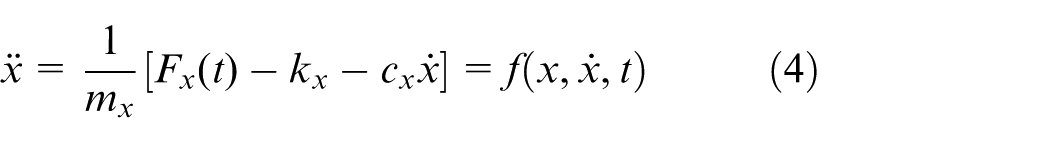
In the flank milling process, the tool has greater stiffness in the axial direction; thus, tool vibration can be defined as a two-degree-of-freedom spring damping vibration system, as shown in Figure 2, and the dynamic analytical model can be derived from equation (1)
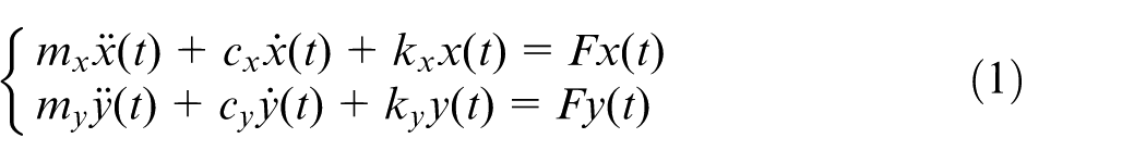
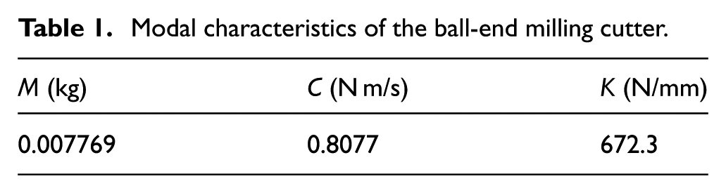
where x(t) and y(t) represent the dynamic displacements at the cutter locations in the X and Y directions, respectively; mx and my denote the mass of the tool in the X and Y directions, respectively; cx and cy denote the damping of the tool in the X and Y directions, respectively; kx and ky denote the stiffness of the tool in the X and Y directions, respectively; and Fx and Fy denote the instantaneous milling force in the X and Y directions, respectively. Table 1 shows the modal characteristics of the milling system obtained via hammer test. 23
Modal characteristics of the ball-end milling cutter.
Model and calculation of the instantaneous milling force
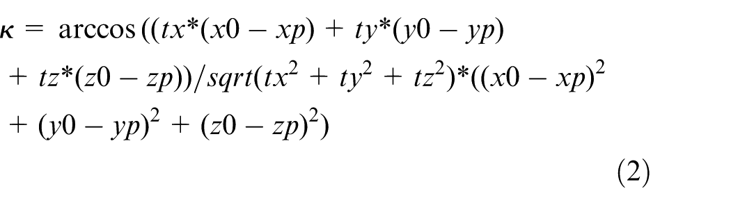
An arbitrary position on the cutting edge of the ball-end mill, which is designated point P, is selected as the origin. The local edge coordinate system P is shown in Figure 3(a). In this figure, dFt(κ), dFr(κ) and dFa(κ) are the tangential, radial and axial force components of the cutting edge element, respectively; κ represents the axial immersion angle, which is π/2 in the flank edge milling process. At the ball-end part of the tool, the tool contact point is assumed to be P(xp, yp, zp) at a given time; the tool center point is O(x0, y0, z0); and the tool axis vector is V(tx, ty, tz). Then, the axial immersion angle can be expressed as shown in equation (2)
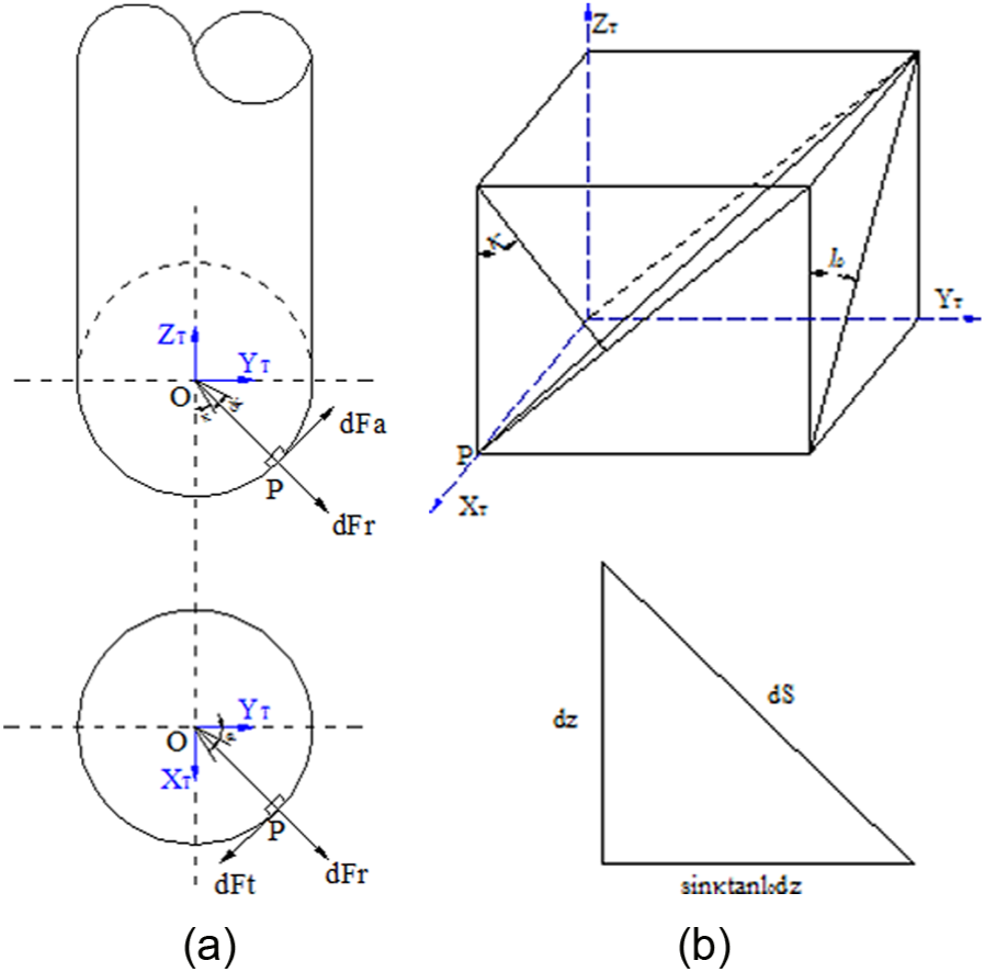
Local coordinate system and differential element length calculation: (a) milling force components and (b) differential element length.
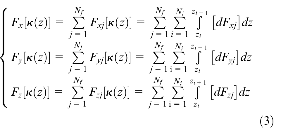
The instantaneous milling force in the three directions can be expressed as shown in equation (3)
where
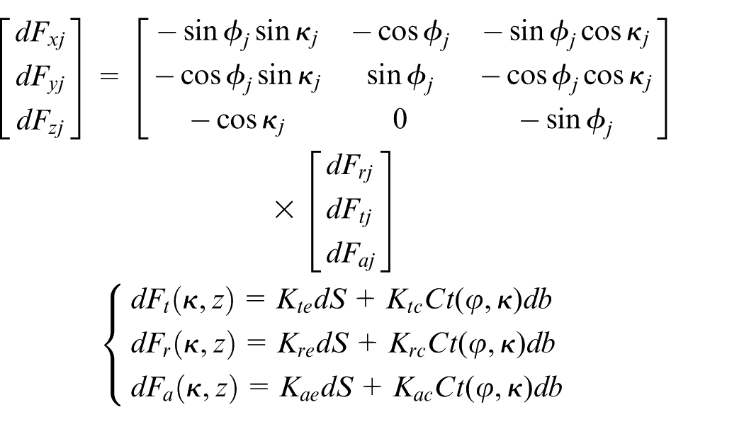
To calculate the cutting forces
In this study, the average cutting force of each tooth was used to calibrate the milling force coefficient, and the geometric shape and dimensions of the workpiece used to test the average cutting force are shown in Figure 4.
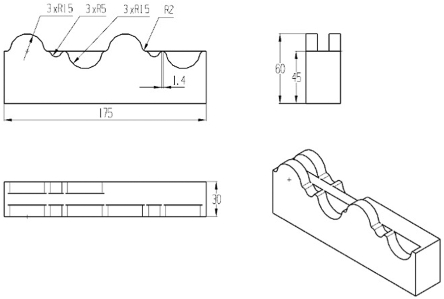
Geometric shape and dimensions of the workpiece.
The experimental scheme is as follows:
Perform the flank milling operation to the first set of convex and concave teeth; the teeth have a radius of 15 mm with a feed per tooth of 0.05 mm/t and a fixed cutting depth.
Perform the flank milling operation to the second set of convex and concave teeth; the teeth have a radius of 15 mm with a feed per tooth of 0.10 mm/t and a fixed cutting depth.
Perform the flank milling operation to the third set of convex and concave teeth; the teeth have a radius of 15 mm with a feed per tooth of 0.15 mm/t and a fixed cutting depth.
The average milling force was obtained from the instantaneous cutting force measured by the dynamometer. The processing site is shown in Figure 5.
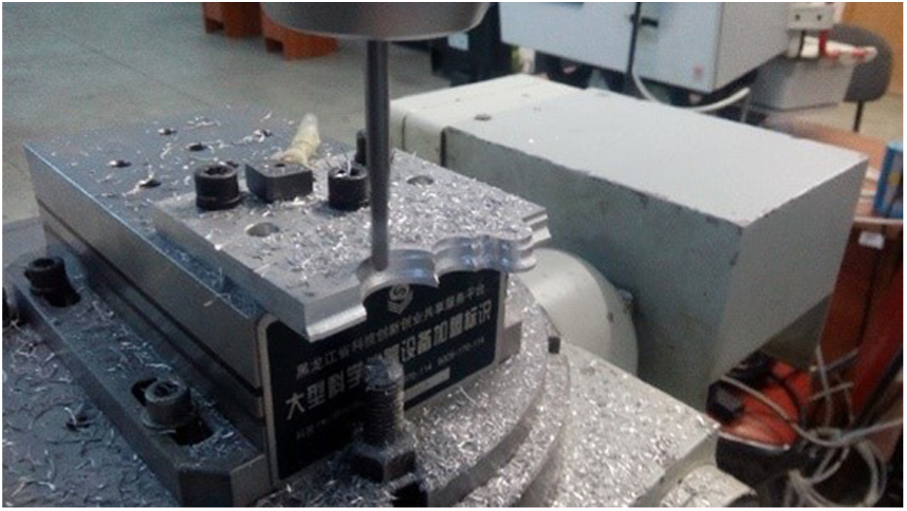
Cutting force coefficient experiments.
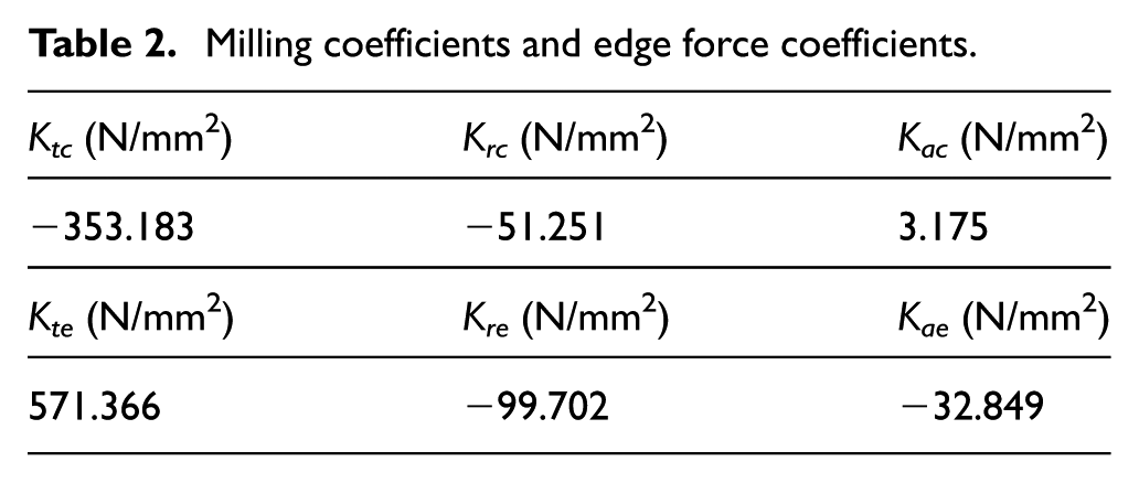
Considering the zero drift data of the dynamometer in the process of idle tool-path machining, the milling force data obtained from the experiments were processed and input into the milling force coefficient calculation models. Table 2 shows the milling coefficients and edge force coefficients that were obtained.
Milling coefficients and edge force coefficients.
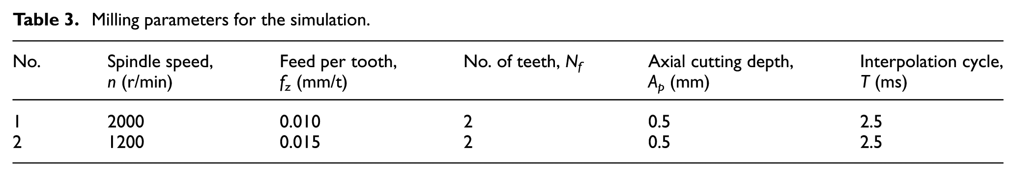
The milling forces for a ruled surface blade were simulated for the milling parameters shown in Table 3 (No. 1 relates to the suction surface and No. 2 relates to the pressure surface). Figures 6 and 7 present the milling forces under conditions No. 1 and No. 2, respectively. The simulation of the pressure surface in the machining process proceeds from the bottom of the impeller to the top, whereas the simulation of the suction surface proceeds from top to bottom.
Milling parameters for the simulation.
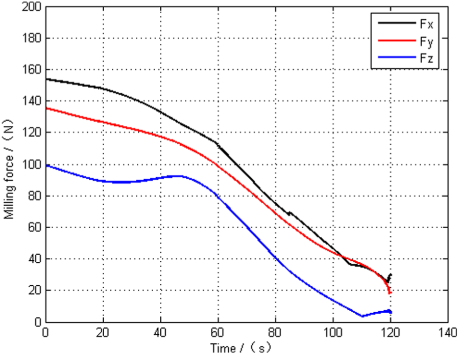
Milling forces of the suction surface.
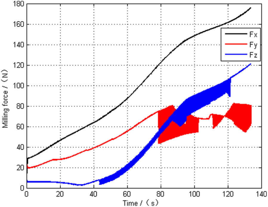
Milling forces of the pressure surface.
Solution and simulation of the dynamic displacements of the flexible cutter
Most previous publications used the Euler method to solve the time-domain differential equation. However, the Euler method is a simple one-step method that has difficulty solving the second-order differential equation and cannot guarantee the accuracy of the solution. In this article, the solution process used to solve differential equations in the time domain is based on the fourth-order Runge–Kutta method, which is a single step method with greater solution accuracy and stability than the Euler method. However, the classical fourth-order Runge–Kutta method can only calculate the first-order differential equation. Therefore, this study uses an intermediate variable to transform the second-order differential equation into a first-order differential equation before performing the calculations. Taking the solution process for the dynamic displacements in the X direction as an example, this method requires that the time step dt remains sufficiently small to ensure the accuracy of the solution. Similarly, the calculation in the Y direction is also solved according to the following process:
The second-order differential equation is rewritten as a first-order differential equation that can be solved using the Runge–Kutta method, and an intermediate variable is constructed to transform the equation into the form of vibration acceleration. The intermediate variable is derived from equation (1) as
The tool rotation period is divided into N equally sized periods. N must be sufficiently large to ensure that the discrete time period is sufficiently small.
From t = 0, the time increases by the small step size dt, which is substituted into the instantaneous milling force Fx(t) at the response moments and then calculated over the entire processing time. Each discrete time point of the vibration displacement, velocity and acceleration is successively calculated according to this method.
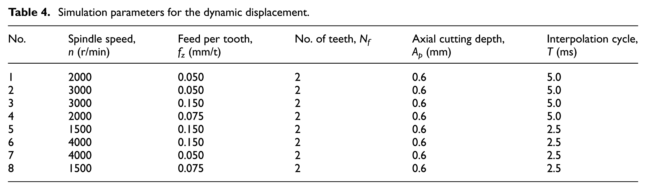
Following the above calculation method, VC++ programming and MATLAB software were used to simulate the dynamic displacement in the flank milling process for a ruled surface. Figures 8 and 9 show the machining state and simulation process, respectively. The simulation of the pressure surface in the machining process proceeds from the bottom of the impeller to the top, whereas the simulation of the suction surface proceeds from the top to bottom. The simulation parameters of dynamic displacement are shown in Table 4 (Nos 1–4 relate to the suction surface and Nos 5–8 relate to the pressure surface).
Simulation parameters for the dynamic displacement.
Ruled surface impeller in flank milling.
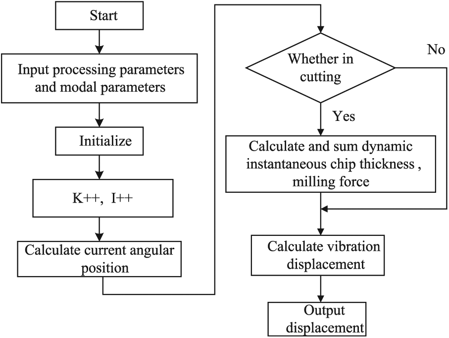
Process for simulating the dynamic displacement.
Taking the parameters of Nos 3 and 5 listed in Table 4 as an example, the simulation results for the dynamic displacement are shown in Figures 10 and 11.
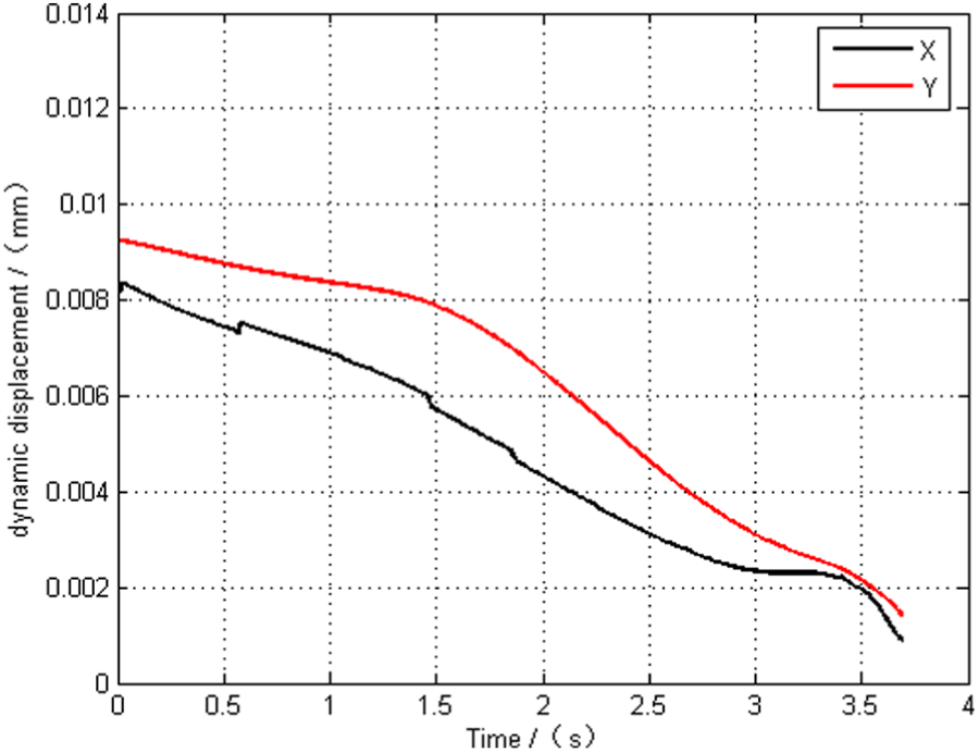
Third group of dynamic displacements.
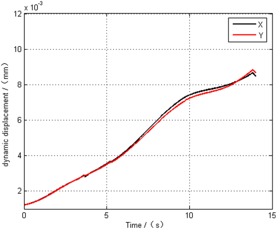
Fifth group of dynamic displacements.
In Figure 10, the dynamic displacement exhibits a decreasing trend during the processing of the suction surfaces. This decreasing trend is consistent with the feeding trajectory characteristics, which transits from a large axial cutting depth to a small cutting depth on the suction surface blade. A smaller cutting depth results in a smaller dynamic milling force between the tool and the blade, resulting in a smaller dynamic displacement. According to the dynamic displacements under the conditions of Nos 1–4 listed in Table 4, for a given feed per tooth, with increasing spindle speed, the dynamic displacement in the X direction decreases compared to the Y direction. For a given spindle speed, as the feed per tooth increases, the dynamic displacement in the Y direction decreases. At the same time, the difference between the dynamic displacement in the X and Y directions increases.
In Figure 11, the dynamic displacement exhibits an increasing trend during the processing of the pressure surfaces, which is consistent with the feeding trajectory characteristics that transition from a small axial cutting depth to a large axial cutting depth on the pressure surface blade. The dynamic displacement in the X direction shifts from larger to smaller than that in the Y direction, under the conditions of Nos 5 and 6. The dynamic displacements in both directions decrease, but for a given feed per tooth, the difference in displacement increases with increasing spindle speed. At the same time, the difference between the dynamic displacement in the X and Y directions increases. For a given spindle speed, the dynamic displacement in the Y direction remains largely unchanged, and the displacement in the X direction decreases as the feed per tooth increases, under the conditions of Nos 6 and 7 (as in Nos 7 and 8).
The amplitude and characteristics of the tool dynamic displacement in the X and Y directions differ with varying milling parameters. This difference reflects the different vibration characteristics in the processing.
Deformation analysis of the flexible tool in flank milling
Because the cutter used in flank milling has a long cantilever, it also experiences deformation during the machining process, which results in various problems, such as machining errors and insufficient surface precision. Therefore, the tool deformation must be predicted, and its deformation trend must be analyzed. In this study, ANSYS is used to analyze the deformation of the cylindrical ball-end milling cutter at different times in the flank milling process of a ruled surface blade. The milling force can be obtained using the milling force calculation method, and the responding cutter deformation can be analyzed after inputting the milling force into ANSYS. The following assumptions must be made before studying and analyzing the deformation of the flexible tool:
The performance of the workpiece and cutting tool is constant and does not vary with temperature or other factors in the machining process.
There is no plastic deformation during the process, and all of the deformations are caused by the milling force.
The milling cutter has no abrasion and is clamped without eccentricity; thus, the results of the previous force simulation can be used for the deformation analysis.
Pre-processing of the finite element model of the ball-end milling cutter
A geometry model of the ball-end cylindrical milling cutter is created, and its geometric parameters are set according to the parameters of the milling cutter. The milling cutter is made from cemented carbide, and its performance indicators are shown in Table 5. The cylindrical ball-end milling cutter model is created in the UG environment and then imported into ANSYS using the x_t format.
Performance indicators for cemented carbide.
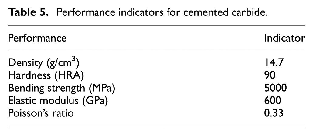
After the ball-end milling tool model is imported into ANSYS, the material properties of the corresponding cutter are set according to the performance indicators of cemented carbide in Table 5. Then, this set of material properties is applied to the entire milling cutter, and the grid mesh of the integral cutting tool is generated. Based on the analysis of the mesh grid quality, the final finite element model is established with 23,847 nodes and 15,343 units.
The constraint type at the root of the milling cutter is set as all constraints. The remaining parameters are set as follows: spindle speed of 2100 r/min, feed per tooth of 0.015 mm/t, tool radius of 3 mm and milling allowance of 0.5 mm. A total of 10 different time points in the machining process are selected to analyze the bending deformation of the milling tool. According to the dynamic milling force measured in Figure 12 (the experiment site is shown in Figure 8), the milling forces at separate time points can be selected and input along two edges of the ball-end milling cutter in the form of a uniformly distributed load. Figure 12(b) shows that the rotation frequency is 35 Hz and that the cutting frequency is 70 Hz. In addition, there is a slightly unsteady cutting frequency at 60 Hz. Finally, the tool deformations at the different time points are analyzed individually until all of the points in the selected processing path have been considered.
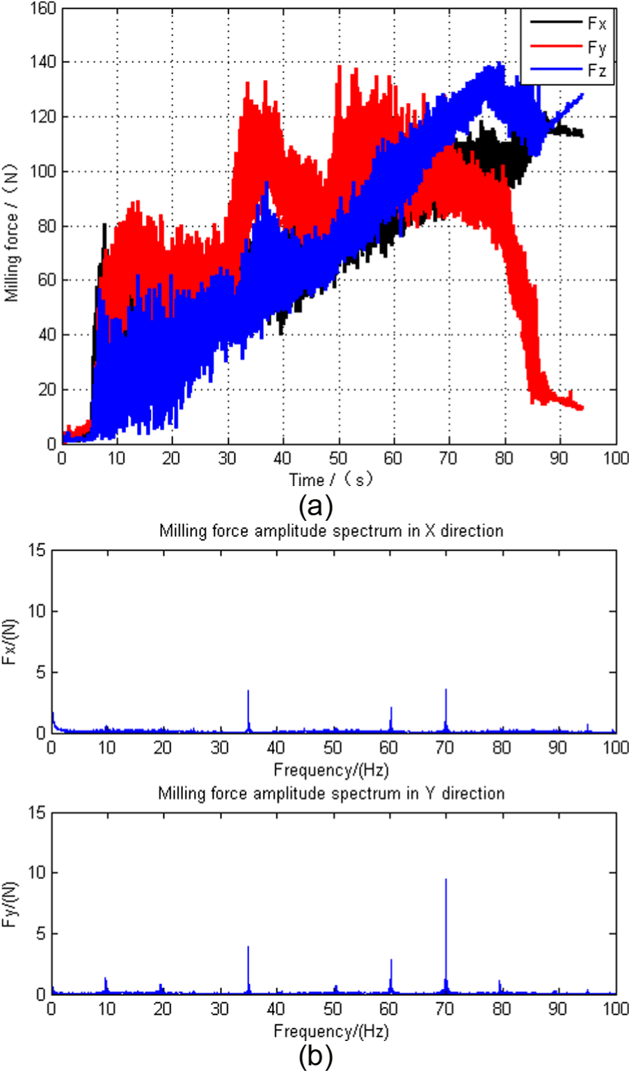
Milling force characteristics for the pressure blade: (a) time-domain characteristics of the milling forces and (b) frequency-domain characteristics of the milling forces.
Post-processing for the finite element model of the ball-end milling cutter
The deformation nephogram in Figure 13 shows that the tool deformation varies based on the cutter location under the influence of a dynamic milling force. For example, the cutting tool root exhibits no deformation, and the tip of the tool is the location of maximum deformation. The deformations in the tip area of the cutting tool are often larger than the deformations in the root area. Specifically, the deformation reaches its peak value at the location of the largest curvature variation.
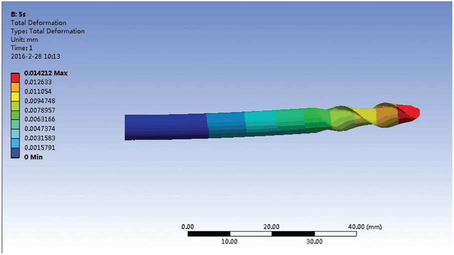
Deformation nephograms at 40 s.
According to the post-processing results, the maximum deformations at various time points are collected and fitted to a curve, as shown in Figure 14. The maximum deformation area of the cylindrical ball-end milling cutter occurred at the cutter tip on the pressure surface from the root of the impeller to the top. The maximum and minimum deformation values are 0.0296 and 0.0039 mm, respectively.
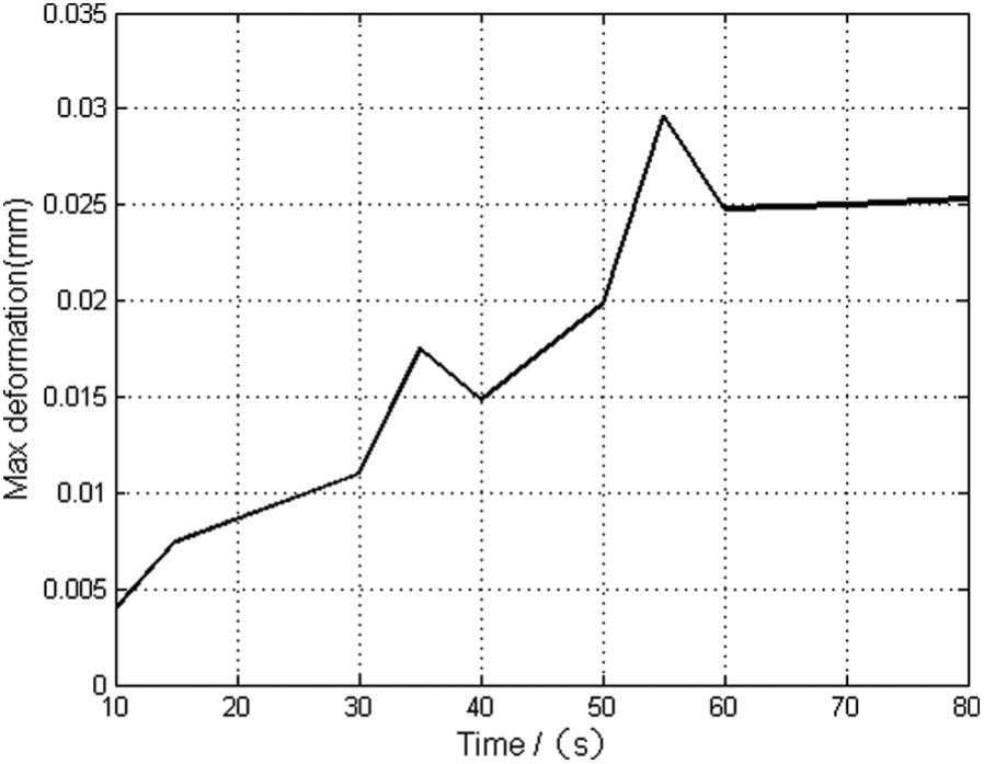
Maximum deformation curve at various time points.
The milling tool is acted on by three forces from different directions and exhibits deformation when the cutter mills the pressure surface. The data in Figure 14 illustrate that in the machining process of milling the impeller from its root to its top, the maximum deformation of the cutter gradually increases during the first 35 s and then decreases slightly after 40 s, possibly due to the curvature fluctuation of the blade. From 40 to 55 s, the deformation begins to gradually increase, and after 55 s, the deformation decreases again, which corresponds to the second largest curvature fluctuation of the blade. After this point, the maximum deformation does not exhibit large variations until the end of the process.
Optimization of the milling parameters based on the dynamic response of the milling system
The dynamic response of the milling system affects the machining quality of the blades. The dynamic displacement simulation results presented above illustrate that the machining parameters have a significant influence on the dynamic response. Thus, in this section, an intelligent optimization method is proposed based on the dynamic response of the cutter in the process of the milling the pressure surface. Various parameters are optimized, including the spindle speed, feed per tooth and milling allowance.
Design of the optimization experiment
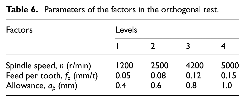
Based on the simulations, the dynamic displacement responses of the system comprising different factors and different levels are obtained to train a neural network model. In the simulation, before optimizing the parameters, the feasible range of each parameter is confirmed by considering the actual machining capacity. Then, simulation experiments are performed according to orthogonal design. The parameter values are chosen according to the different factors and levels shown in Table 6, and 16 groups’ simulated displacement results are obtained with the corresponding parameters. For example, maximal displacement in the X direction is 0.1471 mm, and maximal displacement in the Y direction is 0.0812 mm under the condition of 2500 r/min, 0.15 mm/t and 0.8 mm allowance.
Parameters of the factors in the orthogonal test.
Neural network prediction model
This study uses the BP neural network method to consider the effects of spindle speed, feed per tooth and milling allowance on the dynamic displacement. Therefore, the input layer has three neurons based on the number of parameters to be optimized. The output layer contains two neurons, which denote the maximum displacements in the X and Y directions. Based on the learning rate of the entire network and repeated testing, the number of implicit layer neurons is determined to be 15 according to the Kolmogorov’s theorem. The ultimate BP network structure in this article is 3 × 15 × 2, as shown in Figure 15.
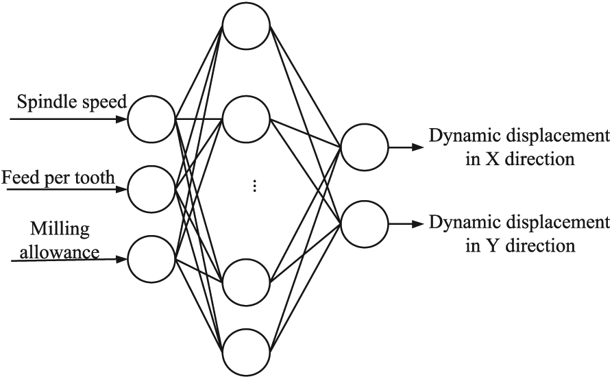
Neural network model.
In 16 groups’ simulated displacement results, the first 14 simulated samples are used to train the network and the remaining two groups serve as a validation sample. The training program is run in VC++, where the target error in the training set is 0.0001. If the error is greater than 0.0001, another group of samples is used to implement the positive spread of the network and the negative spread of the error. All of the samples continue to be used in this manner until the error is less than the target, and the error convergence curve of the network is shown in Figure 16.
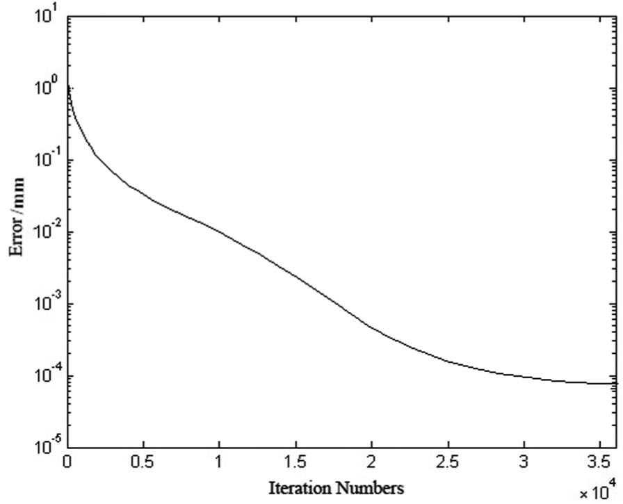
Relationship between the mean square error and the number of iterations.
Particle swarm optimization algorithm for optimizing the milling parameters
Reasonable milling parameters improve the machining quality and stability of the cutting state. Therefore, the five-axis milling process for a ruled surface blade can be defined as a standard optimization that can be solved using a particle swarm optimization algorithm. Before optimizing the parameters, the objective function and constraint condition of the parameters should be satisfied. This section defines the machining optimization model for the aluminum alloy workpiece as

where the constraint conditions are as follows: 1000 r/min < n < 5500 r/min, 0.03 mm/t < fz < 0.15 mm/t and 0.03 mm < ap < 0.12 mm.
Based on the accurate neural network prediction model, the particle swarm optimization algorithm is used to optimize the defined factors. The basic steps of the algorithm are as follows:
The particle number N is set as 80, the inertia weight ω is set as 0.4 and the cognitive coefficient and social coefficient are set as c1 = c2 = 2.07. The initial position and velocity of each particle are set randomly within these constraint conditions, and the best position for an individual particle is set as the original position. Among the optimal individual positions, the best individual position is set as the best position of the swarm.
Predict the individual position of each particle using the network model. If the new value is better than the previous optimal individual position, the former optimal individual position is replaced; if the new value is better than the current best position of the swarm, the optimal swarm position will also be updated.
Update the position and velocity of the particles according to equations (6) and (7).
Set the total number of iterations to 200. If the number of iterations cannot reach that value, then process returns to step 2. If the number of iterations exceeds 200, then stop the algorithm and output the optimal solution
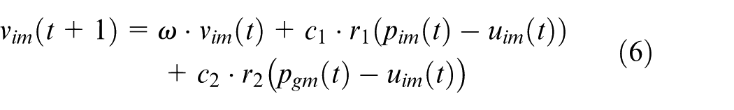

where
The optimization algorithm presented in this article is shown in Figure 17. The relationship between the optimal target, namely, the optimal swarm solution, and the number of iterations is shown in Figure 18.
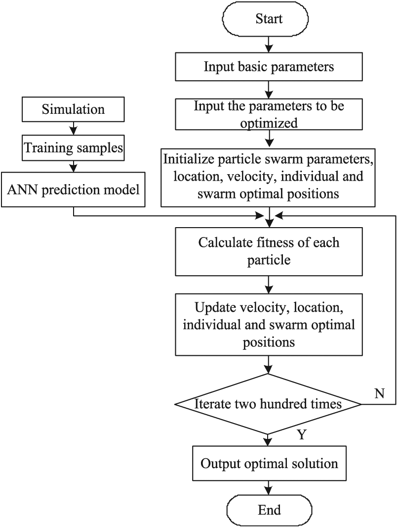
Neural network–particle swarm optimization process.
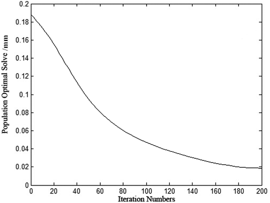
Relationship between the optimal swarm solution and the number of iterations.
Finally, the optimized spindle speed is 4865 r/min, the optimized feed per tooth is 0.1 mm/t and the optimized milling allowance is 0.9 mm. Comparing the experimental results of the milling pressure surface with the optimized parameters and the orthogonal experiment parameters (4200 r/min, 0.05 mm/t, 0.8 mm) illustrates that the machining process with optimized parameters results in a higher surface quality of the blade. Thus, the optimization algorithm is effective. The results for the machined surfaces are shown in Figure 19.
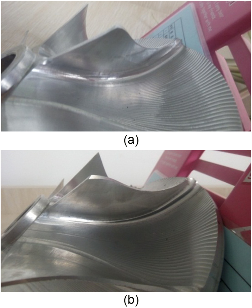
Machined pressure surfaces of the blades: (a) before optimization and (b) after optimization.
To compare the machined surface qualities of the two pressure surfaces, the SRT6200 surface roughness tester shown in Figure 20 was used to measure these two blades. Five well-proportioned areas of each blade were measured from bottom to top, and the tester measured an area of 2.5 mm (blade tip to blade root) each time. The test results are shown in Figure 21.
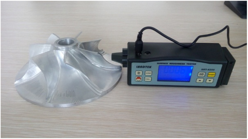
SRT6200 surface roughness tester.
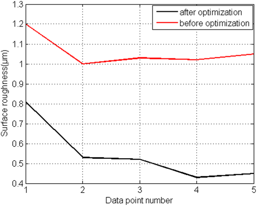
Surface roughness of the blades before and after optimization.
This figure shows that the overall surface roughness decreases after optimization, with a maximum reduction of approximately 2.5 times. After optimization, the spindle speed and the feed per tooth both increase, which decreases the milling force between the tool and the workpiece. This effect is helpful for reducing the dynamic displacement of the tool and improving the surface quality of the workpiece. The roughness values before and after optimization show similar trends. The maximum surface roughness occurs at the base of the impeller pressure surface. This result is possibly due to the volatility in the curvature during the processing of this part and the rapidly spinning machine C axis reducing the processing quality. The large impact is the main reason for the increase in the surface roughness, as the tool mills the pressure surface starting from the base.
Conclusion
This study analyzed the dynamic displacement response and optimized the processing parameters for a ruled surface impeller in the flank milling process. The following conclusions can be drawn:
The dynamic response model for the milling cutter was constructed. The dynamic displacement of the cutter was simulated according to the milling force calculated at each cutter location during the processing of the ruled surface blade. The dynamic displacement was analyzed with different machining parameters, and the results showed that the dynamic displacements increased in the X and Y directions from the bottom to the top of the impeller pressure surface during the machining process. In addition, a relatively large displacement change rate appears at the position with the largest variation curvature of the blade.
The deformation on a ball-end cutter was analyzed for a machining path with certain machining parameters using ANSYS. The measured dynamic milling forces were input onto the cutting edge of the finite element model of a ball-end milling cutter, and the deformation nephograms of the cutter at each processing time were obtained. The analysis indicated that the maximum deformation of the milling cutter is 0.0296 mm at the position of the maximum curvature variation of the blade.
A method combining a BP neural network and particle swarm optimization algorithm was proposed. The machining parameters and maximum dynamic displacement of the cutter were used as training samples to train the BP neural network, and the maximum dynamic displacement of the cutter was taken as the optimization objective. Then, the trained neural network was used as a criterion to evaluate the individual and swarm optimal solutions. Finally, a machining experiment was conducted with the optimized parameters to validate the proposed method. The surface roughness test results indicated that the optimized parameters can effectively reduce the surface roughness of the pressure surface and improve the surface quality of the machined blade.
Footnotes
Appendix 1
Declaration of conflicting interests
The author(s) declared no potential conflicts of interest with respect to the research, authorship and/or publication of this article.
Funding
The author(s) disclosed receipt of the following financial support for the research, authorship, and/or publication of this article: This study was supported by the Natural Science Foundation of China (Grant No. 51205098) and Natural Science Foundation of Heilongjiang Province of China (Project No. QC2016069).